Examination of wind speed based on field measurements on a low-rise building

Mean and peak wind speeds, as well as gust factors, integral scales, and intensity of turbulence values, are essential in formulating wind loading standards for structures. In recent years, the characterization of rooftop wind speeds has become more important when designing photovoltaic arrays. As part of an investigation into the wind loading and structural behavior of pedestal mounted photovoltaic arrays, wind speeds at two elevations were investigated through an analysis of field measurements performed at the Central Washington University campus in Ellensburg, Washington. Specifically, two roof-mounted R.M. Young ultrasonic anemometers were employed in the data collection project: one located at 21.9 m [72 ft] above ground, and the other, closer to a pedestal-mounted photovoltaic array, at 12.5 m [41 ft] above ground. The wind speeds measured by the 21.9 m elevation anemometer were examined with a view to ascertaining that they are not significantly affected by the Central Washington building sited near its location. This paper focuses on the examination of the wind speeds only. Results showed that the wind speeds measured by the 12.5 m elevation anemometer are significantly affected by the presence of the building and that significant resonant effects are induced for the photovoltaic panels. The results of this work make it possible to adopt Japanese structural design practice wherein the design is performed for wind effects induced by 10-min, rather than by 60-min wind speeds as in current U.S. practice, thereby significantly reducing computation times. The results presented in this work also allow for the rigorous determination of 10-min speeds as functions of peak 3-s gusts. Estimates of integral scales of turbulence were shown to be characterized by large uncertainties, on the basis of which it is possible to obtain coefficients of variation required for determining the magnitude of wind load factors used in practice.

1 Introduction

Several studies have been performed for in situ measurements of wind speeds and pressures for low-rise buildings (Levitan et al., 1991; Cochran and Cermak, 1992; Okada and Ha, 1992). Due to the large number of roofing failures under extreme winds, a significant amount of research on determining pressures on rooftops has recently been performed, as reported in other studies (Martins et al., 2016; Baskaran et al., 2018). Results of wind tunnel tests of photovoltaic systems have already been reported previously (Kopp and Banks, 2012; Kopp, 2013; Stenabaugh et al., 2015; SEAOC Solar Photovoltaic Systems Committee, 2017; Naeiji et al., 2017), a majority of them for ground-mounted rather than roof-top panels. Studies are scarce on evaluating the impact of wind effects on roof-mounted photovoltaic panels as per the Minimum Design Loads and Associated Criteria for Buildings and Other Structures (ASCE/SEI 7-22) (American Society of Civil Engineers, 2022). The current study undertakes an in-depth analysis of in-situ wind velocities affecting roof-top photovoltaic panels. Two anemometers were installed at different elevations and different distances from a neighboring building. It was observed that the wind speeds measured by one of the anemometers were not unaffected by the presence of that building. Wind speed time series were obtained as part of an ongoing project aimed at characterizing wind loadings and the structural behavior of full-scale in situ rooftop pedestal-mounted photovoltaic systems (Bender et al., 2018; Estephan, 2021).

The following section elaborates on the data collection and includes the results of computations aimed at estimating uncertainties in the estimation of flow parameters (turbulence intensity, integral turbulence scale, and turbulence spectra). Based on the principle that wind speed fluctuations in free flow are normally distributed, an approach is presented to determine wind speeds averaged over time intervals different from one hour, as functions of peak (3-s) wind speeds, length of time series record, and roughness of terrain. This approach could help supersede U.S. practice wherein 60-min time series are considered in structural design and to adopt the Japanese practice wherein 10-min time series are considered instead. Thus, the proposed method helps substantially reduce computational durations for the design of a wide class of structures. Overall, the wind speed data acquired in this project can be used for the validation of various computational fluid dynamics calculations.

2 Materials and methods

2.1 Data collection

In 2021, time-series wind speed data were collected as part of a collaborative effort between three US universities: Florida International University (FIU), Central Washington University (CWU), and the University of Washington (UW) to investigate the modeling of full-scale wind pressure loadings on pedestal-mounted rooftop photovoltaic arrays. The instrumented low-rise building, Hogue Hall, is located on the Central Washington campus in Ellensburg, Washington. Hogue Hall is rectangular in shape with nominal dimensions of 12 m [40 ft] height, 42 m [138 ft] width, and 56 m [184 ft] length with a rooftop parapet wall height of 825 mm [2.7 ft]. A close-up aerial view of Hogue Hall is provided in Figure 1A. The campus surroundings are low-rise buildings, tennis courts, and parking lots as depicted in Figure 1B.

Figure 1

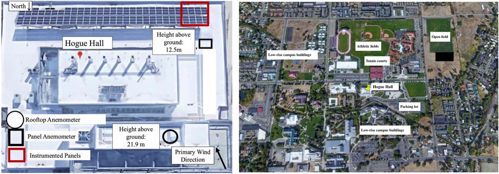
Figure 1. (A) Aerial view of the rooftop of Hogue with location of anemometers identified. Source: Google Earth. (B) Aerial view of Hogue with surroundings. Source: Google Earth.

The focus of this paper is the wind speed measurements recorded by the two R.M. Young ultrasonic anemometers, models 85,000 and 86,000, at 21.9 m [72 ft] and 12.5 m [41 ft], respectively, as shown in Figure 1A. They are labeled as “rooftop” and “panel” anemometers because the lower one was installed in front of the photovoltaic panel array to capture the wind speeds closer in location to the panels. Presumably, this anemometer would have been in the disturbed shear flow created by the building itself. The rooftop anemometer was placed on a 2.82 m [9 ft 3 in] tripod on the roof on the front or north side of the building. Metal ties secured the tripod. Data were collected at the maximum recording frequency of 122 Hz for the rooftop and 25 Hz for the panel anemometer.

The collected wind data time series were provided to LabVIEW. The data collection is set to start after 120 s of consistent wind speed over 4.46 m/s [10 mph] and stop after 120 s of consistent wind under 4.46 m/s [10 mph]. Acquisition and storage of data were done through National Instruments cRIO controllers. The purpose of installing the real-time controllers was to acquire and store data remotely on-site, without any need to directly connect to a primary computer. The real-time controllers were connected to the primary computer via the LAN network. This enabled a user to remotely modify and observe the real-time program on the controller and then remotely download the data collected after a test without having to physically retrieve the controllers’ flash drives. Each controller had various data acquisition modules installed to which the sensors were connected. In the next section, parameters used for data analysis are defined.

2.2 Data Analysis

The turbulence intensity I_u is the ratio of the standard deviation of the wind speed fluctuations to the mean wind speed:

$I_u=\frac{{\sigma }_u}{\overline{U}.}(1)$

where σ_u is the standard deviation and $\overline{U}$ is the mean.

This parameter provides a measure of the magnitude of the velocity fluctuations relative to the mean wind speed. Another important statistical parameter is the gust factor G_U. It is important to convert wind speeds from a short time duration to a longer one, such as the conversion from a 3-s gust U₃ to an hourly value U_hourly or vice-versa. The ratio of the wind speed U_t averaged over t seconds to that over 3,600 s (i.e., 1 h) is defined as the gust factor G_U:

$G_U=\frac{U_t}{U_{hourly}}=\frac{U_{t\left[\mathit{sec}\right].}}{U_{3600}}(2)$

Typically, these types of conversions are undertaken using the Durst formulation for gust factors (American Society of Civil Engineers, 2022; Durst, 1960). However, the Durst model is limited to open terrain conditions and installed at a height of 10 m above ground. Investigations for other terrain conditions have been undertaken in recent years in numerous studies (Wieringa, 1973; Greenway, 1979; ESDU 83045, 1983; Ashcroft, 1994; Kareem and Zhou, 2003; Kwon and Kareem, 2014). Wieringa (1973) evaluated gust factors over a lake and at the edge of a town. The gust factor was found to be associated with surface roughness and height above ground. Ashcroft (1994) investigated the influence of terrain roughness and mean wind speed on the gust factor and documented that the gust ratio is influenced by the terrain roughness though he did not report a general pattern of change for ratios and the increasing wind speed. Engineering Sciences Data Unit or ESDU (ESDU 83045, 1983) investigated the variation of mean-hourly wind speeds for various terrain conditions and their influence on gust factors. Krayer and Marshall evaluated different gust factors for hurricane records and reported that an upward adjustment from the existing Durst gust values was appropriate (Krayer and Marshall, 1992). They also concluded that a closer examination of the probability distribution function of the gust factors was in order. Schroeder and Smith (2003) evaluated wind flow characteristics for Hurricane Bonnie and had findings similar to those by Krayer and Marshall. Schroeder and Smith observed greater energy in the low-frequency region of the longitudinal power spectrum than that predicted in earlier analytical models, and corresponding discrepancies in the estimation of integral scales. Masters (2004) examined gust factors for tropical cyclone data and corroborated the robustness of the Krayer-Marshall models, i.e., larger gust factors than the Durst values. Yu and Chowdhury (2009) examined gust factors for the Florida Coastal Monitoring Program (FCMP) tropical cyclone data compared with Automated Surface Observing System (ASOS) data for extratropical storms; they reported higher gust factors supporting the findings by Krayer and Marshall. They highlighted the importance of further study on thermal stratification to assess the influence of temperature on the gusts. Empirical relationships for gust factors for various terrain conditions based on the log law description for wind speed have been established (Simiu, 2011). The current study also aimed to compare these empirical predictions with the in-situ data. In another study (Simiu and Scanlan, 1996) introduced a formulation was introduced for modifying the Durst equation for other terrains and hurricane wind speeds using the logarithmic law with correction factors. The equation for G_U is as follows:

$G_U=\frac{U_t\left(z\right)}{U_{mean}\left(z\right)}=1+\frac{\eta \left(z_0\right)c\left(t\right)}{2.5\mathit{ln}\left(\frac{z}{z_0}\right),}(3)$

where η(z₀) denotes a factor for surface roughness and c(t) is a factor for averaging time.

ESDU 83045 (ESDU 83045, 1983) makes use of a peak factor g, the mean velocity U, and the turbulence intensity I_u as follows, in its definition of the gust factor:

$G_U\left[aka{K}_{\tau }\right]=\frac{\widehat{U}\left(t,T_0\right)}{U}=\frac{U\left(t,T_0\right)+\widehat{u}\left(t,T_0\right)}{U}=1+g{I}_u,(4)$

where T₀ is the time interval within which wind speed applies or the observation period over which wind speed is measured and $\widehat{u}$ is a peak value.

While the peak factor g can be estimated from measured data, the ESDU document has formulated a methodology for estimating the second term in Equation 4 based on different gust averaging times (t). The following equations apply in this formulation:

$g=\frac{\widehat{u}\left(t,T_0\right)}{{\sigma }_u\left(t,T_0\right)}*\frac{{\sigma }_u\left(t,T_0\right)}{{\sigma }_u}.(5)$

$\frac{\widehat{u}\left(t,T_0\right)}{{\sigma }_u\left(t,T_0\right)}=\sqrt{2\mathit{ln}\left[T_0\nu \left(t,T_0\right)\right]}+\frac{0.577}{\sqrt{2\mathit{ln}\left[T_0\nu \left(t,T_0\right)\right].}}(6)$

$T_u=3.13z^{0.2}\mathrm{s}\mathrm{e}\mathrm{c}\mathrm{o}\mathrm{n}\mathrm{d}\mathrm{s}.(7)$

$\frac{{\sigma }_u\left(t,T_0=1\mathrm{h}\mathrm{o}\mathrm{u}\mathrm{r}\right)}{{\sigma }_u}=1-0.193{\left[\frac{T_u}{t}+0.1\right]}^{-0.68}.(8)$

$\nu \left(t,T_0=1\mathrm{h}\mathrm{o}\mathrm{u}\mathrm{r}\right)=\frac{0.007+0.213{\left(\raisebox{1ex}{$T_u$}\!\left/ \!\raisebox{-1ex}{$t$}\right.\right)}^{0.654}.}{T_u}(9)$

where T_u = the integral time scale; z = height above ground; t = gust averaging time; $\widehat{u}$ = peak value.

Liu et al. (2021) examined the ASCE7 gust effect or response factor for rigid buildings in conjunction with the aerodynamic admittance function. The gust factor is a component of the ASCE7 formulation of the gust response factor for buildings, which separates the low and high-frequency contributions of the wind speed spectrum from the corresponding pressure loadings. As the low-frequency region remains poorly understood, the Standard is expected to benefit from further investigation into the wind spectrum.

Various formulations for wind spectra exist in the literature (Simiu and Scanlan, 1996). Although ESDU 74030 and 74,031 (ESDU, 1974a; ESDU, 1974b) use the von Karman expression to characterize wind velocities, the Kaimal expression has been found more appropriate (Simiu, 2011). The Kaimal expression for the spectrum S_u at height z above ground is represented as under (Simiu and Scanlan, 1996):

$\frac{n{S}_u\left(z,n\right)}{u_{*}^2}=\frac{200f}{{\left(1+50f\right)}^{\raisebox{1ex}{$5$}\!\left/ \!\raisebox{-1ex}{$3$}\right.}}.(10)$

where $f=\raisebox{1ex}{$nz$}\!\left/ \!\raisebox{-1ex}{$\overline{U}(z)$}\right.$; n is frequency in Hz; $\overline{U}$(z,n) is the mean wind speed; u_* is the friction velocity.

The integral scale of turbulence ^xL_u is defined as the integration of the autocovariance function R_u as follows, e.g., (Simiu and Scanlan, 1996)

${}^x{L}_u=\overline{U}{\displaystyle \underset{0}{\overset{\infty }{\int }}}\frac{R_u\left(\tau \right)}{{\sigma }_u^2}d\tau =\overline{U}{\displaystyle \underset{0}{\overset{\infty }{\int }}}{\rho }_u\left(\tau \right)d\tau .(11)$

where $R_u\left(\tau \right)$ is the autocovariance function; ${\rho }_u\left(\tau \right)$ is the autocorrelation; τ is the time lag.

Because the autocovariance R_u is the Fourier transform of the spectrum S_u, the following equation is employed to determine ^xL_u, e.g., (Simiu and Scanlan, 1996)

${}^x{L}_u=\frac{\overline{U}{S}_u\left(n\cong 0\right)}{4{\sigma }_u^2}.(12)$

Equation 12 implies that knowledge of the lower-frequency region is critical for estimating the integral scale of turbulence.

The method attributed to Davenport and Solari (Davenport and Dalgliesh, 1971; Solari, 1993a; Solari, 1993b; Solari and Kareem, 1998) for determining the influence of the wind spectrum on the gust factor and loading of structures, has been defined by the following set of equations (Solari, 1993a; Solari, 1993b):

$G_U=1+g_u{I}_u\sqrt{P_0,}(13)$

$g_u\cong {\left\{1.175+2\ln \left[\stackrel{\sim }{t}\sqrt{\frac{P_1}{P_0}}\right]\right\}}^{\raisebox{1ex}{$1$}\!\left/ \!\raisebox{-1ex}{$2$}\right.},(14)$

$P_0={\displaystyle \underset{0}{\overset{\infty }{\int }}}\frac{S_u\left(n\right)}{{\sigma }_u^2}X\left(n,\overline{\tau }\right)dn,(15)$

$X\left(n,\overline{\tau }\right)=\frac{{\mathit{sin}}^2\pi n\overline{\tau },}{{\left(\pi n\overline{\tau }\right)}^2}(16)$

$P_1={\displaystyle \underset{0}{\overset{\infty }{\int }}}{\left[\frac{n{}^{x}L_u}{\overline{U}}\right]}^2\frac{S_u\left(n\right)}{{\sigma }_u^2}X\left(n,\overline{\tau }\right)dn,(17)$

$\stackrel{\sim }{t}=\frac{T\overline{U}}{{}^{x}L_u.}(18)$

where g_u = peak factor; I_u = turbulence intensity; n = frequency in Hz; ${}^{x}L_u$ = integral scale of turbulence; S_u = wind speed spectrum; ${\sigma }_u^2$ = variance of wind speed; $\overline{U}$ = mean wind speed; T = time duration over which the wind speed is averaged; $\overline{\tau }$ = the averaging time of the peak gust.

As a peak value, G_U can be fitted by an extreme value distribution. The equation for the probability density function y associated with the generalized extreme value distribution for x is

$y=f\left(x|k,\mu ,\sigma \right)=\left(\frac{1}{\sigma }\right)\mathit{exp}\left(-{\left(1+k\frac{\left(x-\mu \right)}{\sigma }\right)}^{-\left(\raisebox{1ex}{$1$}\!\left/ \!\raisebox{-1ex}{$k$}\right.\right)}\right){\left(1+k\frac{\left(x-\mu \right)}{\sigma }\right)}^{-1-\left(\raisebox{1ex}{$1$}\!\left/ \!\raisebox{-1ex}{$k$}\right.\right)},(19)$

where k, μ, and σ are the parameters of the distribution (MATLAB, 2020).

3 Results

3.1 Data processing

Measurements during the windy period yielded 94 1-h time series records. The rooftop anemometer recorded slightly more data than the panel because the mean wind speed surpassed the set point of 4.46 m/s more often. Furthermore, each 1-h record for the wind speed data consisted of approximately 90,000 (panel) to 440,000 (roof) observations; the number varies due to the 25 Hz recording for the panel anemometer and 122 Hz for the rooftop one. The directionality of the data was checked to examine any large deviations in wind direction through wind roses. The wind roses were fitted to mean wind directions for the records. The site exhibits a strong directionality in the NW quadrant with the angles being between 325–340° as shown in the wind rose of Figure 2. Hence, using each 1-h record for its entirety was considered appropriate.

Figure 2

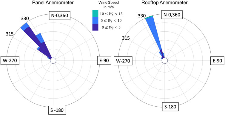
Figure 2. Wind roses for the anemometer data.

Stationarity tests were undertaken for the hour-long records. Visual inspection of the hour-long records showed storms with small or no changes to the mean value. When fitting a linear regression model to the mean as a function of time, the slope was found close to 0. The substantial number of observations proved somewhat problematic for stationarity testing. That is, tabulated values are provided for observations much smaller than 90,000. The Augmented Dickey-Fuller test was used on hour-long storms with the highest mean values, e.g., (MATLAB, 2020). For these records, the p-value was 0.045 (<0.05) with a test statistic of −1.986 and a critical value of −1.942 for a significance level of 5%. Resultantly, the Augmented Dickey Fuller test confirmed weak stationarity for the records. In order to compare results with previous investigations, the hourly data sets were initially separated into subsets of over four hundred 15-min (900 s) packets. These data sets are examined in the next section.

3.2 Measured wind flow characteristics

An example of the wind velocity time series data is furnished in Figures 3A, B for the 15-min highest wind speed data for the rooftop and panel data, respectively, for the 25 Hz sampling time. Figures 4A, B depict the corresponding spectra for the time series. The Kaimal spectrum of Equation 10 fitted to the data is shown for comparison. The rooftop data have shown markedly higher energy in the lower frequencies and lesser in the higher frequencies, whereas the panel record appears to have significant energy contributions for a larger range of frequencies.

Figure 3

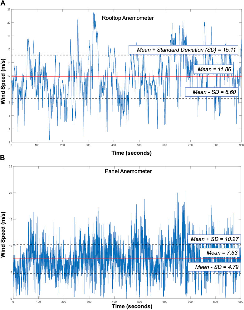
Figure 3. (A) Rooftop anemometer time series. (B) Panel anemometer time series.

Figure 4

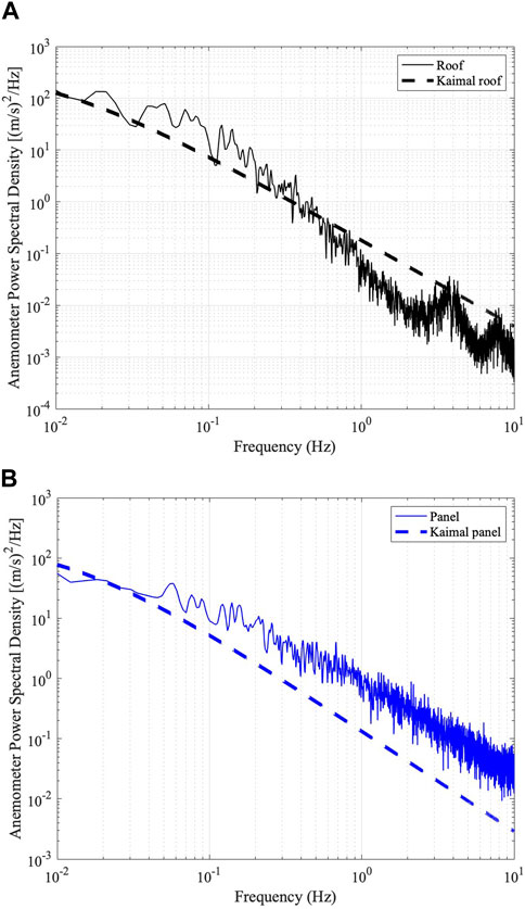
Figure 4. (A) Example spectrum using pwelch (MATLAB, 2020) for the time series in Figure 3A with the Kaimal expression shown. (B) Example spectrum using pwelch (MATLAB, 2020) for the time series in Figure 3B with the Kaimal expression shown.

Figure 5 shows histograms for the mean and maximum wind speeds, as well as the turbulence intensity data for the rooftop and panel. The mean hourly wind speed values ranged from 2 to 7 m/s for the panel and 3 to 12 m/s for the rooftop anemometer. The turbulence intensity I_u, defined in Equation 1 was in the range of 0.15 to 0.53, with the panel anemometer showing higher values. The panel intensities illustrate the disturbance of the wind flow near the panel array in situ. The maximum hourly wind speeds were in the range of 5 to 23 m/s. Using the log law as well as ESDU 83045, the value of the surface roughness parameter z₀ was estimated to be 0.25 m [9.8 in].

Figure 5

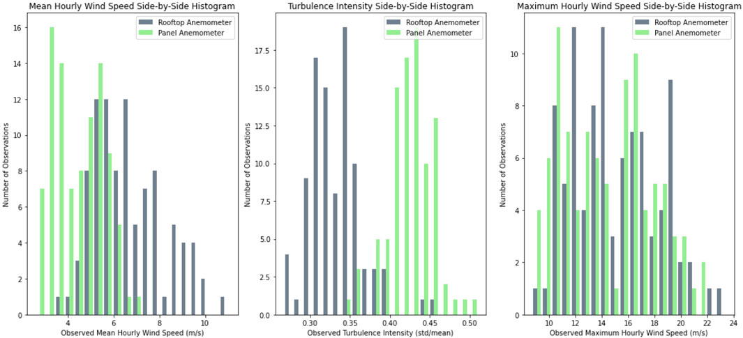
Figure 5. Histograms for the wind speed data.

The intensity of turbulence values I_u were fitted by a normal distribution as shown in Figure 6 for the rooftop and the panel, respectively. The rooftop values ranged from 0.27 to 0.45, with a mean of 0.30 and a coefficient of variation COV of 0.07. For the panel data, the mean value of I_u is 0.39 with a COV of 0.05. The range of values is slightly higher than that for the rooftop, thereby reflecting its position in the disturbed flow region of the lower roof.

Figure 6

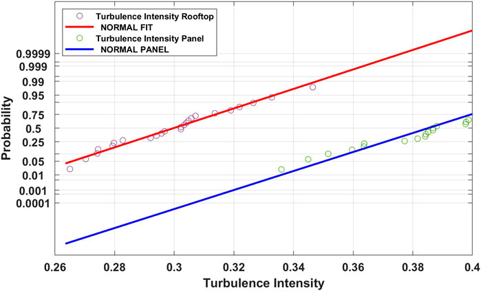
Figure 6. Normal probability plot for the turbulence intensity values for the rooftop and panel. N = 24.

The integral scales ^xL_u were derived from the integration of the autocovariance function as given in Equation 11. The rooftop data results demonstrate an approximate range of 34.6–81 m for ^xL_u. The mean value was 52.1 m, with a COV of 0.24. The values of the integral scales derived from the 15-minute spectra are smaller than the estimate of 106.8 m from ASCE7-22 (American Society of Civil Engineers, 2022). The panel data have a smaller range of values. For the panel data, the mean ^xL_u is 9.2 m with a COV of 0.21. Both were best fitted by normal distributions as shown in Figure 7.

Figure 7

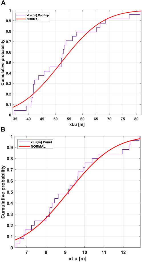
Figure 7. (A, B) Integral scales of turbulence for the rooftop and panel, respectively.

3.3 Gust factor estimation

The data sets were used to determine the gust factor G_U as defined in Equation 2. Because the moving average and segmental approaches to time averaging provided comparable results, the segmental was employed for the records as it was computationally faster. The peak t-second average value for each hour was divided by the mean for that hour. The averaging time t ranged from 0.1 to 3,600 s. These G_U values are shown in Figure 8. The data exhibit a wide scatter for the smaller t values. The rooftop G_U ranged from 1.0 to 2.76 with an average of 1.57 and COV of 0.31. The panel G_U had a maximum of 3.89, with an average of 1.73, and a COV of 0.41. The best fit relationship for the rooftop data as a function of averaging time t in seconds is

$\frac{U_t}{U_{3600}}=2.059t^{-0.089}\mathrm{w}\mathrm{i}\mathrm{t}\mathrm{h}{R}^2=0.8696.(20)$

Figure 8

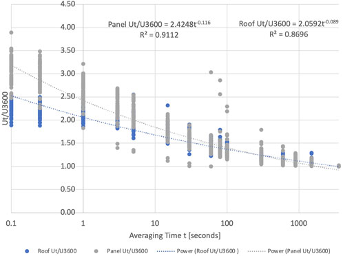
Figure 8. Gust factor plots for the rooftop and panel, respectively.

The panel data have a similar relationship as given in Equation 21:

$\frac{U_t}{U_{3600}}=2.423t^{-0.116}with{R}^2=0.9112.(21)$

3.3.1 Comparison with empirical methods

Equation 3 was evaluated for the rooftop and panel data assuming a z₀ factor of 0.25 m [9.8 in] and the hourly mean wind speed. The results are furnished in Figure 9 along with Equations 20 and 21. In addition, the empirical approximation for the Durst curve is shown in ASCE7-22 (American Society of Civil Engineers, 2022). Gust factor values in the lower averaging times are underestimated by the empirical model.

Figure 9

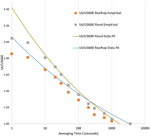
Figure 9. Comparison of data with empirical prediction method in Equation 3.

3.3.2 Extreme value analysis

The U_t/U₃₆₀₀ data for the lower averaging time t values display a wide scatter relative to the larger averaging times. As used in ASCE7 criteria, the 3-s averaging time was evaluated for these data. Table 1 provides some sample statistics for the U₃/U₃₆₀₀ and U₃/U₉₀₀ values for the rooftop and panel, respectively.

Table 1

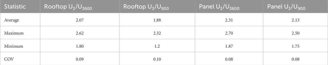
Table 1. Statistics for G_U for 3 s and 15 min. COV = coefficient of variation.

Because the gust factor is a peak value divided by a mean value, the Central Washington measurements provide suitable data for fitting an extreme value distribution. The generalized extreme value (GEV) distribution in MATLAB (MATLAB, 2020) given in Equation 19 was found to be the best fit for U₃/U₉₀₀ and U₃/U₃₆₀₀ as shown in Figure 10, for the rooftop and panel, respectively.

Figure 10

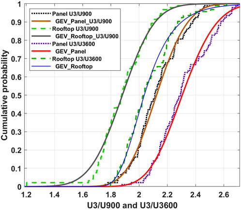
Figure 10. Gust factor distribution fitting. GEV = Generalized Extreme Value. N = 94 observations.

Table 2 provides various distribution parameters for both the hourly and 15-min (900 s) G_U values, which are commonly employed in practice. Other G_U comparisons were made using ESDU 83045 (ESDU 83045, 1983). Equation 4 for the panel data yielded a fitted g of 2.34 for the hourly data. Equations 5–9 were used to determine relationships for the peak factor g for both the U_t/U₉₀₀ and U_t/U₃₆₀₀ data, respectively as shown in Figure 11. Equations 22–25 were found fit to the results. These peak factor values are slightly larger than those determined from the data.

$\mathrm{P}\mathrm{e}\mathrm{a}\mathrm{k}\mathrm{f}\mathrm{a}\mathrm{c}\mathrm{t}\mathrm{o}\mathrm{r}\mathrm{g}\left[\mathrm{r}\mathrm{o}\mathrm{o}\mathrm{f}\mathrm{t}\mathrm{o}\mathrm{p}{\mathrm{U}}_{\mathrm{t}}/{\mathrm{U}}_{3600}\right]=3.4701t^{-0.117},R^2=0.6997.(22)$

$\mathrm{P}\mathrm{e}\mathrm{a}\mathrm{k}\mathrm{f}\mathrm{a}\mathrm{c}\mathrm{t}\mathrm{o}\mathrm{r}\mathrm{g}\left[\mathrm{r}\mathrm{o}\mathrm{o}\mathrm{f}\mathrm{t}\mathrm{o}\mathrm{p}{\mathrm{U}}_{\mathrm{t}}/{\mathrm{U}}_{900}\right]=3.13231t^{-0.123},R^2=0.695.(23)$

$\mathrm{P}\mathrm{e}\mathrm{a}\mathrm{k}\mathrm{f}\mathrm{a}\mathrm{c}\mathrm{t}\mathrm{o}\mathrm{r}\mathrm{g}\left[\mathrm{p}\mathrm{a}\mathrm{n}\mathrm{e}\mathrm{l}{\mathrm{U}}_{\mathrm{t}}/{\mathrm{U}}_{3600}\right]=3.5341t^{-0.141},R^2=0.8322.(24)$

$\mathrm{P}\mathrm{e}\mathrm{a}\mathrm{k}\mathrm{f}\mathrm{a}\mathrm{c}\mathrm{t}\mathrm{o}\mathrm{r}\mathrm{g}\left[\mathrm{p}\mathrm{a}\mathrm{n}\mathrm{e}\mathrm{l}{\mathrm{U}}_{\mathrm{t}}/{\mathrm{U}}_{900}\right]=3.2056t^{-0.15},R^2=0.8446.(25)$

Table 2

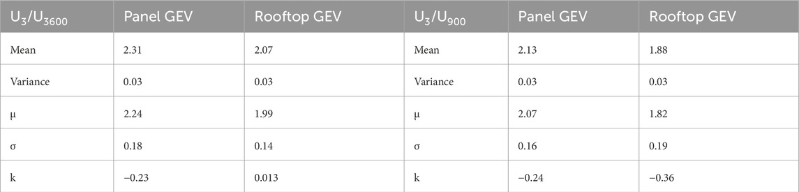
Table 2. Generalized Extreme Value (GEV) parameters for gust factors from Equation 19.

Figure 11

Figure 11. ESDU 83045 data fits for the peak factor g.

The method attributed to Davenport and Solari (D-S) e.g., (Solari, 1993a; Solari, 1993b) as shown in Equations 13–18 was investigated for the rooftop and panel data. For this method, the rooftop mean G_U was 1.79 with associated mean g_u = 3.01, which matches the ESDU estimate. The mean values of the other parameters were P₀ = 0.77; P₁ = 0.07; I_u = 0.30; and wind speed = 10 m/s. These G_U values were close to the mean U₃/U₃₆₀₀ of 1.74 for the in situ records. The panel data resulted in Davenport-Solari values of mean G_U = 1.87 with mean g_u = 3.16, which is higher than the mean G_U = 2.10 from the data. The mean values of the other parameters were P₀ = 0.51; P₁ = 0.01; I_u = 0.39; and wind speed = 6.3 m/s.

4 Discussion

Analysis of the spectral content for both data sets identified differences in the low and high-frequency ranges. The Kaimal spectrum was a good fit for the rooftop spectrum overall, although the rapid drop-off in the higher frequency range for the data was unexpected. It is suggested to conduct more studies in future. The spectral content for the panel anemometer located in a disturbed flow region displayed energy contributions for both low and high frequency regions. As expected, the spectrum is not representative of the Kaimal expression and illustrates the effects of the building itself. In addition, the energy content in the high-frequency range for the panel anemometer may indicate the possibility of wind-induced vibrations (dynamic response) of the photovoltaic arrays corresponding to the system’s natural frequencies. The corresponding lower integral scale of turbulence values indicates that a lower spatial correlation exists in the disturbed flow region. The large turbulence intensities for the panel also reflect the disturbed wind flow in that section of the roof. The turbulence intensity and integral scales of turbulence parameters were found to be Normal variables, with COV values of about 20%. This level of uncertainty seems reasonable for in situ conditions.

Gust factors for the rooftop and panel locations had similar trends in overall averaging times, with both locations displaying a large scatter for lower t values. The measured sparse suburban values were larger than those for open terrain as expected. Generalized extreme value distributions provided good fits for both anemometers and simplified the process of determining extreme values for the sparse suburban conditions for given probability levels.

The entire formulation of the ASCE7 gust response factor calculations, even for rigid buildings, depends upon the gust factor G_U, the wind spectrum S_u(n), and the integral scale of turbulence ^xL_u. Notably, the COV for gust factors in the lower averaging times is about 30%, which suggests that the suggested gust response factor of 0.85 for rigid buildings may not be as conservative as assumed.

5 Conclusion

Wind speed field measurements from two ultrasonic anemometers mounted on a low-rise building were presented and discussed. The Kaimal spectrum was a good fit to the rooftop data overall, with the measured data displaying a more rapid drop-off in the higher frequency range than expected. The panel spectra exhibited energy over a larger range of frequencies, which is indicative of the disturbed flow region. The high energy content in the high-frequency range of the spectrum can lead to wind-induced dynamic effects on the photovoltaic systems (which is a topic of future research). It was found that the gust factors display a wide scatter for low t values when plotted against the averaging time t. A generalized extreme value distribution was fit to the U₃/U₃₆₀₀ and U₃/U₉₀₀ ratios for both anemometers. The integral scale of turbulence and the turbulence intensity were best fit by Normal distributions. The corresponding ASCE7-22 integral scale value was much higher than the field data, suggesting a greater correlation than in situ.

Data availability statement

The raw data supporting the conclusions of this article will be made available by the authors, without undue reservation.

Author contributions

SW: writing–original draft and writing–review and editing. DR: conceptualization, formal analysis, funding acquisition, methodology, supervision, writing–original draft, writing–review and editing, data curation, investigation, and resources. GL: methodology, software, writing–original draft, and writing–review and editing. JE: methodology, software, and writing–review and editing. PI: conceptualization, formal analysis, investigation, methodology, software, supervision, and writing–review and editing. AC: conceptualization, data curation, formal analysis, investigation, methodology, project administration, software, supervision, validation, writing–original draft, and writing–review and editing.

Funding

The author(s) declare that financial support was received for the research, authorship, and/or publication of this article. The writers acknowledge the National Science Foundation (NSF) for collaborative research awards 1824995 and 1825908 to FIU, and CWU and UW.

Conflict of interest

The authors declare that the research was conducted in the absence of any commercial or financial relationships that could be construed as a potential conflict of interest.

Publisher’s note

All claims expressed in this article are solely those of the authors and do not necessarily represent those of their affiliated organizations, or those of the publisher, the editors and the reviewers. Any product that may be evaluated in this article, or claim that may be made by its manufacturer, is not guaranteed or endorsed by the publisher.

Author disclaimer

The views and opinions expressed in this paper are those of the writers and do not necessarily reflect the position of the NSF.

References

Ashcroft, J. (1994). The relationship between the gust ratio, terrain roughness, gust duration and the hourly mean wind speed. JWEIA 53, 331–355. doi:10.1016/0167-6105(94)90090-6

CrossRef Full Text | Google Scholar

Baskaran, A., Molleti, S., Martins, N., and Martin-Perez, B. (2018). Development of wind load criteria for commercial roof edge metals. J. Archit. Eng. 24. doi:10.1061/(asce)ae.1943-5568.0000308

CrossRef Full Text | Google Scholar

Bender, W., Waytuck, D., Wang, S., and Reed, D. A. (2018). In situ measurement of wind pressure loadings on pedestal style rooftop photovoltaic panels. Eng. Struct. 163, 281–293. doi:10.1016/j.engstruct.2018.02.021

CrossRef Full Text | Google Scholar

Cochran, L. S., and Cermak, J. E. (1992). Full- and model-scale cladding pressures on the Texas Tech University experimental building. J. Wind Eng. Industrial Aerodynamics 43 (1), 1589–1600. doi:10.1016/0167-6105(92)90374-j

CrossRef Full Text | Google Scholar

SEAOC Solar Photovoltaic Systems Committee (2017). Wind design for solar arrays. California: Structural Engineers Association of California.

Google Scholar

Davenport, A. G., and Dalgliesh, W. A. (1971). “A preliminary appraisal of wind loading concepts of the 1970 National Building Code of Canada,” in Third international conference on wind effects on buildings and structures. Tokyo, Japan.

Google Scholar

Durst, C. S. (1960). Wind speeds over short periods of time. Meteorological Mag. 89 (1056), 181–186.

Google Scholar

American Society of Civil Engineers, (2022). Minimum design loads and associated criteria for buildings and other structures. ASCE.

Google Scholar

ESDU (1974a). Characteristics of atmospheric turbulence near the ground Part 1 ESDU. Charlotte St., London, UK: Engineering Sciences Data Unit Ltd.: Hartford House, 7–9.

Google Scholar

ESDU (1974b). Characteristics of atmospheric Turbulence near the ground Part II, ESDU. London, UK: Engineering Sciences Data Unit Ltd.

Google Scholar

Greenway, M. E. (1979). An analytical approach to wind velocity gust factors. JWEIA 5, 61–91. doi:10.1016/0167-6105(79)90025-4

CrossRef Full Text | Google Scholar

Kareem, A., and Zhou, Y. (2003). Gust loading factor—past, present and future. JWEIA 91, 1301–1328. doi:10.1016/j.jweia.2003.09.003

CrossRef Full Text | Google Scholar

Kopp, G. A. (2013). Wind loads on low profile, tilted, solar arrays placed on large, flat low-rise building roofs. J Struct Engr.

Google Scholar

Kopp, G. A., and Banks, D. (2012). Use of the wind tunnel test method for obtaining design wind loads on roof-mounted solar arrays. J. Struct. Engr. doi:10.1061/(ASCE)ST.1943-541X.0000654

CrossRef Full Text | Google Scholar

Krayer, W. R., and Marshall, R. D. (1992). Gust factors applied to hurricane winds. Bull. Am. Meteorological Soc. 73, 613–618. doi:10.1175/1520-0477(1992)073<0613:gfathw>2.0.co;2

CrossRef Full Text | Google Scholar

Kwon, D. K., and Kareem, A. (2014). Revisiting gust averaging time and gust effect factor in ASCE7. J. Struct. Engr. 140 (11). doi:10.1061/(asce)st.1943-541x.0001102

CrossRef Full Text | Google Scholar

Levitan, M. L., Mehta, K. C., Vann, W. P., and Holmes, J. D. (1991). Field measurements of pressures on the Texas tech building. J. Wind Eng. Industrial Aerodynamics 38, 227–234. doi:10.1016/0167-6105(91)90043-v

CrossRef Full Text | Google Scholar

Liu, Y., Kopp, G. A., and Chen, S.-f. (2021). An examination of the gust effect factor for rigid high-rise buildings. Front. Built Environ. 6 (February). doi:10.3389/fbuil.2020.620071

CrossRef Full Text | Google Scholar

Martins, N. E., Martin-Perez, B., and Baskaran, A. (2016). Application of statistical models to predict roof edge suctions based on wind speed. JWEIA 150, 42–53. doi:10.1016/j.jweia.2016.01.003

CrossRef Full Text | Google Scholar

Masters, F. J. (2004). Measurement, modeling and simulation of ground-level tropical cyclone winds. ProQuest Dissertations & Theses. University of Florida, 3145950.

Google Scholar

MATLAB (2020). MATLAB programming language.

Google Scholar

Naeiji, A., Raji, F., and Zisis, I. (2017). Wind loads on residential scale rooftop photovoltaic panels. JWEIA 168, 228–246. doi:10.1016/j.jweia.2017.06.006

CrossRef Full Text | Google Scholar

Okada, H., and Ha, Y.-C. (1992). Comparison of wind tunnel and full-scale pressure measurement tests on the Texas Texh Building. J. Wind Eng. Industrial Aerodynamics 43 (1), 1601–1612. doi:10.1016/0167-6105(92)90375-k

CrossRef Full Text | Google Scholar

Estephan, J. (2021). “Peak wind effects on low-rise building roofs and rooftop PV arrays,” in 6th American association for wind engineering workshop. Editor N. Kaye (Clemson University). (online).

Google Scholar

ESDU 83045, (1983). Strong winds in the atmospheric boundary layer 83045. Engineering Sciences Data Unit, 30.

Google Scholar

Schroeder, J. L., and Smith, D. A. (2003). Hurricane Bonnie wind flow characteristics as determined from WEMITE. J. Wind Eng. Industrial Aerodynamics 91, 767–789. doi:10.1016/s0167-6105(02)00475-0

CrossRef Full Text | Google Scholar

Simiu, E. (2011). Design of buildings for wind: a guide for ASCE7-10 standard users and designers of special structures. Second ed. Hoboken, New Jersey: John Wiley and Sons, 338.

CrossRef Full Text | Google Scholar

Simiu, E., and Scanlan, R. H. (1996). Wind effects on structures. NY,NY: John Wiley and Sons.

Google Scholar

Solari, G. (1993a). Gust Buffeting I: peak wind velocity and equivalent pressure. J. Struct. Engr. 119 (2), 365–382. doi:10.1061/(asce)0733-9445(1993)119:2(365)

CrossRef Full Text | Google Scholar

Solari, G. (1993b). Gust buffeting. II: dynamic alongwind response. J. Struct. Engr. 119 (2), 383–398. doi:10.1061/(asce)0733-9445(1993)119:2(383)

CrossRef Full Text | Google Scholar

Solari, G., and Kareem, A. (1998). On the formulation of ASCE7-95 gust effect factor. JWEIA 77-78, 673–684. doi:10.1016/s0167-6105(98)00182-2

CrossRef Full Text | Google Scholar

Stenabaugh, S. E., Iida, Y., Kopp, G. A., and Karava, P. (2015). Wind loads on photovoltaic arrays mounted parallel to sloped roofs on low-rise buildings. JWEIA 139, 16–26. doi:10.1016/j.jweia.2015.01.007

CrossRef Full Text | Google Scholar

Wieringa, J. (1973). Gust factors over open water and built-up country. Bound. Layer. Meteorol. 3, 424–441. doi:10.1007/bf01034986

CrossRef Full Text | Google Scholar

Yu, B., and Chowdhury, A. G. (2009). Gust factors and turbulence intensities for the tropical cyclone environment. J. Appl. Meteorology Climatol. 48 (3), 534–552. doi:10.1175/2008jamc1906.1

CrossRef Full Text | Google Scholar