 W. Saeger
 P. Miranda
 G. Toledo
 C. E. Silva
 A. Ozdagli
 F. Moreu
- 1Department of Civil, Construction and Environmental Engineering, The University of New Mexico, Albuquerque, NM, United States
- 2Facultad de Ingeniería Mecánica y Ciencias de la Producción, Escuela Superior Politécnica del Litoral, ESPOL, Guayaquil, Ecuador
- 3Department of Mechanical Engineering, The University of New Mexico, Albuquerque, NM, United States
- 4Department of Bioengineering, Civil Engineering, and Environmental Engineering, Florida Gulf Coast University, Fort Myers, FL, United States
Real-time hybrid simulation has gained popularity over the last 20 years as a viable and cost-effective method of testing dynamic systems that cannot be tested using traditional methods. The emergence of multi-axial Real-time Hybrid Simulation (maRTHS) has led to an increase in the allowable fidelity of the numerical and experimental substructures. The testing community can now replicate multiple-degree-of-freedom (MDOF) responses of both substructures and thus can perform more representative tests. However, with this increased fidelity of the substructures comes an increased complexity of controlling these components. Specifically, multi-axial hydraulic actuator assemblages require nonlinear coordinate transformations to derive plant displacements as the force transducers on the actuators are not capable of performing this task directly. Recently, benchmark problems have been provided to the RTHS community in the form of virtual simulations. Virtual simulation refers to a fully virtual testing methodology where numerical and physical components are represented virtually. This approach enables the RTHS community to evaluate various control algorithms without the need to recreate physical components. This project aims to demonstrate the capability of computer vision-based displacement tracking in a realistic virtual simulation of the experimental substructure in avoiding excess nonlinear coordinate transforms. The tracking algorithm utilizing the Lucas-Kanade optical flow method is tested in the virtual simulation environment which is set up using real-time 3D creation engine, Unreal Engine 4 (UE4), and computer graphics software, Blender. This environment interfaces with MATLAB/Simulink, more specifically “Simulation Tool for v-maRTHS benchmark” developed for multi-axial tests. The result of this study establishes a novel framework for applying computer vision-based tracking algorithms and sensing in v-maRTHS simulations using simulated cameras within virtual simulation environments. A computer vision displacement tracking algorithm is developed and optimized to work in tandem with a MIMO PI controller to reduce tracking time delays within 31.25 milliseconds while tracking the nodal displacement and rotation of the frame within a normalized RMSE of 1.24 and 1.10 respectively.
1 Introduction
Real-time hybrid simulation (RTHS) is an experimental technique popularly used to test structural systems that are not typically feasible to implement in a lab setup due to size or cost constraints. Hybrid simulation as we know it today was developed by Hakuno et al. (1969), who used an analog computer to solve a one-degree-of-freedom (1DOF) equation. This novel research on pseudo dynamic (PsD) testing constituted an efficient way of modeling engineering systems and opened the door to developing new experiments with physical and numerical substructures. The first formal contribution to this alternative was formally made by Takashima (Takanashi et al., 1975) in 1975, where the equation of motion (EOM) was discretized in the time domain to facilitate its numerical integration. The substructuring idea arose from these early developments. Substructuring implies that instead of building the entire reference structure for testing, only a portion of it can be extracted as a specimen and tested, focusing on the portion with the most uncertain or hysteretic behavior occurs (Shao et al., 2011; Nakata et al., 2014). On the other hand, Horiuchi et al. (1999) demonstrated in a test of a stiffness specimen that the effect of the time delay is equivalent to adding a negative damping to the structure in RTHS. When this negative damping is greater than or equal to the system damping, instability problems can occur and further threaten the safety of the system.
Due to this effect in RTHS systems, new advanced control strategies have been proposed that seek to minimize the unavoidable delay between the commanded signal and the measured signal. Recently, many of these approaches adapt several stages for robust and adaptive design (Ou et al., 2015; Li et al., 2021), which also increases their attention to improving system performance in the presence of noise and random disturbances.
In efforts to successfully synchronize the experimental and numerical substructures, many sophisticated control algorithms have been developed. To date, in the maRTHS context, robust and adaptive methods (Aguila et al., 2024; Xu et al., 2024) have been proposed to mitigate the inherent unknown uncertainties of the servo-hydraulic system. It has been shown that Linear Quadratic Gaussian (LQG) controllers produce very low tracking errors in single axis RTHS applications (Fermandois, 2019; Wang et al., 2019). These LQG controllers leverage model-based compensation techniques to be robust to model uncertainties. Consequently, compensation methods have emerged obtaining very good results using optimized PI controllers. Tao and Mercan (Tao and Mercan, 2019), optimized their PI controller using an adaptive feedback compensation method. Niño Hilarion, A. (Niño Hilarión, 2021), used a deep learning framework to optimize their PI controller.
Typically, a physical substructure of an RTHS experiment is comprised of a transfer system [servo-valve dynamics, actuator dynamics and control-structure interaction (CSI) (Palacio-Betancur and Gutierrez Soto, 2022)] coupled to an experimental substructure, which is a representation of the full structure (Condori et al., 2023). These components must be properly identified in the form of transfer functions or state-space equations so they can be numerically integrated. However, these dynamics are affected by several factors, such as D/A (digital/analog) and A/D conversions, communication time, controller sampling frequency and actuator dynamics (Dyke et al., 1995), making the successful synchronization of the experimental and numerical substructure a challenge.
Typical control architectures used for conducting RTHS experiments may include feedback signals of displacement, acceleration, and force. Displacement transducers, such as LVDTs, can be used to provide direct displacement measurements of the actuators and the frame. For some laboratory setups it may be difficult or impossible to position or angle the displacement to properly obtain the desired frame displacement measurements. Force-transducers offer an almost instant feedback signal that is optimal for actuator controller purposes and has little structural interaction. However, these sensors are less optimal for determining the nodal displacement of the frame. To find the nodal displacement values the signals received from the force transducers must be converted through a nonlinear coordinate transform, a process in which errors may occur. Additionally, if imperfections exist within the actuator assemblages or the frame itself, there may be uncertainties if the coordinate transform is correctly calculating the nodal displacements of the frame. Accelerometers can also be a solution to get a more exact measurement of the nodal displacement. However, given the need to integrate the signal twice to obtain displacement, their use is prone to producing errors and uncertainties associated with the integration itself and high frequency noise amplification. There are still unanswered questions about using acceleration for RTHS feedback, but contributions by researchers like Liu et al. (2023), and Ferrero et al., (Ferrero et al., 2016), where correction techniques based on Kalman filters are used to reduce these errors have been important to increase the use of acceleration feedback control in RTHS. Computer vision displacement tracking offers a possible solution to these issues by providing a non-contact solution that is unaffected by assemblage or frame uncertainties.
Computer vision-based tracking algorithms have gained popularity over the past 40 years, but little has been done in the context of real-time displacement tracking of structures in the laboratory. Optical Flow is one of the most used and accepted tracking methods. Summarized by Barron et al. (1992), there are many different approaches to applying optical flow methods. Lucas and Kanade and Horn and Schunck all found success using first-order Differential-Based Methods to minimize spatial gradients and estimate normal velocities (Barron et al., 1992). Nagel, Uras, Girosi, Verri, and Torre all found success using second-order Differential-Based Methods. Anandan and Singh utilized Region-Based Matching methods for their optical flow algorithms (Barron et al., 1992). Waxman, Wu, and Bergholm developed a Phase-Based technique that applies spatiotemporal filters to edge maps to track edges in real time (Barron et al., 1992). Fleet and Jepson developed a separate Phase-Based technique that uses band-pass velocity-tuned filters (Barron et al., 1992). Shoa, et al., proposed an advanced binocular vision system for 3D vibration displacement measurements that found success (Ali et al., 2019).
Recently, there has been additional focus on optimizing the Lucas Kanade optical flow computer vision tracking techniques to make them more suitable for real-time displacement tracking. These efforts include creating algorithms that are more robust to noisy measurements and have a reduced processing time (Guo and Zhu, 2016). Aminfar et al. (2019) and Ahmine et al. (2019) investigated the impacts of using Gaussian filters and median filters with different optical flow techniques and were able to achieve much higher spatial resolution within their measurements. Dan et al. (2017) proposed a sparse Lucas Kanade optical flow algorithm through using multi-level pyramids and combining it with the SURF matching algorithm which greatly increased the algorithms tracking speed.
Others have begun using real-time computer vision tracking for control applications. The use of computer vision for control techniques enables one to control numerous points within a camera’s field of view. Manigel and Leonhard used a Kalman Filter and an H2 controller with computer vision to propose new control methods for self-driving cars (Manigel and Leonhard, 1992). Kazemian et al., used computer vision control as a real-time extrusion quality monitoring during robotic building construction (Zisserman and Curwen, 1993).
Recently, there has been an increased focus on developing digital models, consisting of digital twins and simulated cameras that can perform simulations asynchronously with real world sensors. Davis et al. (2024) demonstrated these capabilities by recording the modal shapes of a flexible cantilever beam in a simulation and comparing it to real-world experiments. This project proposes a novel framework to create and evaluate a computer vision displacement tracking algorithm using simulated cameras in a virtual simulation environment for a virtual maRTHS problem.
The structure of this paper is as follows. The subsequent section will discuss the overall methodology of the project. After the methodology, the changes to the Simulink architecture will be discussed. Then, the experimental setup procedure will be detailed in Sections 3–6. This includes the creation process of the virtual-realistic environment, the development of the UE4 and Simulink interface, and finally, the implementation of the computer vision-based displacement tracking algorithm and the MIMO PID controller. Next, the calibration process of the virtual camera and the optimization of the PID controller will be overviewed in Sections 6, 7, respectively. The virtual experiments are detailed in Section 8 followed by analysis of the results of those experiments in Section 9. Conclusions will wrap up this study in Section 10, and followed by Author Contributions, Funding, Acknowledgments, and References.
2 Methodology
To conduct the v-maRTHS simulation for the maRTHS benchmark problem, “Simulation Tool for v-maRTHS benchmark” is utilized. Developed in Simulink, this tool encompasses an all-inclusive RTHS framework with models of the reference structure or ground truth, the numerical substructure, and the experimental substructure. The reference structure is modeled using a SAP2000 finite element model. Both the numerical and experimental substructures are represented as state-space models. The experimental substructure used for this benchmark problem is a frame structure with two S3 × 5.7 columns, a custom-built beam, two connecting joints (Nodes 4 and 7) that bolt the beam to the columns, along with a coupler acting as a transfer system between the actuators and Node 4. The experimental substructure in the lab is depicted in Figure 1 (Condori et al., 2023).
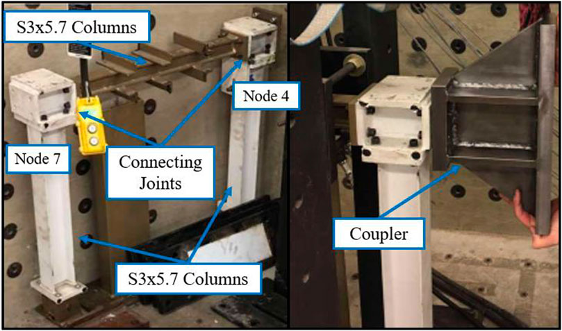
Figure 1. Physical experimental substructure in a laboratory (Condori et al., 2023).
This research aims to create a realistic virtual simulation environment to test and evaluate computer vision-based tracking algorithms. To achieve this goal, the experimental structure is rendered in a real-time 3D creation engine, Unreal Engine 4 (UE4), where the models are built with the Computer Aided Design software SOLIDWORKS, the open-source computer graphics software Blender. Realistic and dimensionally accurate representations of the coupler and the beam are developed in SOLIDWORKS. Blender is employed to model the columns. Finally, UE4 serves as a scaffold for assembling SOLIDWORKS and Blender geometries and for conducting virtual experiments. This process will be discussed in more detail in the subsequent sections. Figure 2 illustrates the data flow of the project.
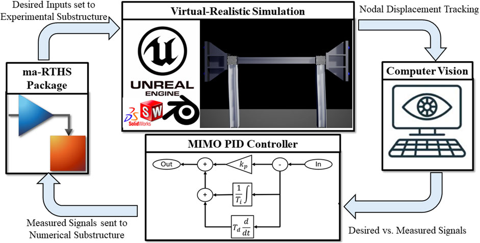
Figure 2. Overview of the v-maRTHS pipeline.
3 Updated Simulink architecture
The Simulink model’s architecture can be divided into three different sub-levels: low-level, mid-level, and high-level. The low-level architecture is defined as the atomic models contained within a block that do not contain any sub-blocks. For example, the experimental substructure representation is low-level, as it does not contain further sub-blocks within itself. Typically, a mid-level block contains only low-level architecture sub-blocks. Here, the controller sub-block is considered mid-level, as it contains the experimental substructure representation along with other low-level blocks such as the Kalman filter. High-level architecture encapsulates all middle- and low-level sub-blocks and coordinates the signals between them.
3.1 Low-level updated architecture
To introduce computer vision capability into the “Simulation Tool for v-maRTHS benchmark” problem, several modifications are made to the Simulink model provided with the benchmark. The representation method of the experimental substructure is changed from a state-space model to a UE4-based virtual-realistic simulation. Four unique modules from the “Vehicle Dynamics Blockset,” “Simulation 3D Actor Transform Set,” “Simulation 3D Actor Transform Get,” “Simulation 3D Scene Configuration,” and “Simulation 3D Camera Get,” are leveraged to enable the virtual simulation. Additionally a separate “MATLAB Function” module is developed to facilitate the computer vision tracking algorithm. Each of these modules will be discussed in detail in later sections. Figure 3 illustrates the “Flexible UE4 Model” sub-block, which includes the new blocks used for computer vision capability.

Figure 3. Vehicle Dynamics Block set modules used for Simulink and UE4 Interface.
3.2 Mid-level updated architecture
The major modification made to the mid-Level architecture of the Simulink model is the addition of measured nodal displacement signals outputting from the “Flexible UE4 Model” sub-block. Mimicking the provided model, these measured actuator signals are sent through an estimator and used in the control loop while also output from the controller sub-block. Additionally, the measured nodal displacement values are also output from the controller sub-block. The actuator displacements are sent through the provided coordinate transformation sub-block and recorded to provide a baseline for comparing the tracking abilities of the computer vision algorithm. These processes can be seen in Figure 4.
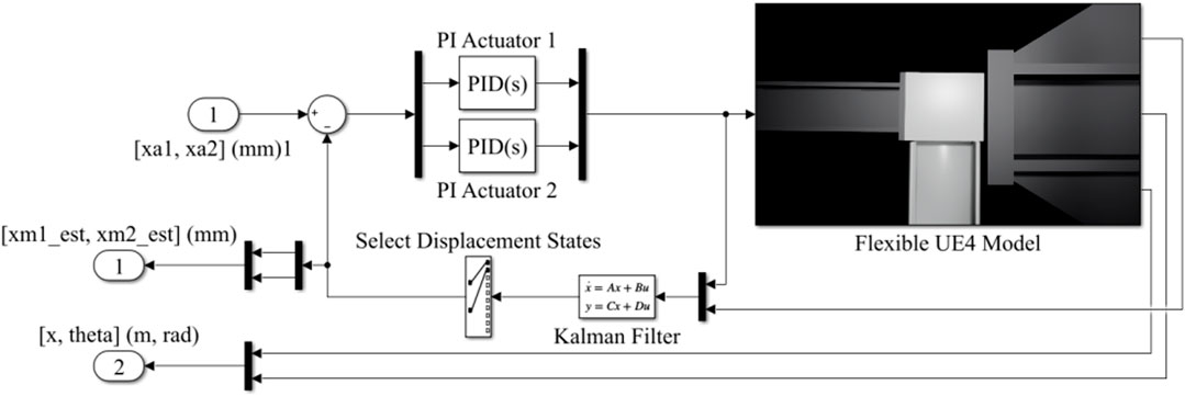
Figure 4. MIMO PID control loop in Simulink.
3.3 High-level updated architecture
The aforementioned mid-level and low-level adjustments are packaged in the “Physical Substructure” sub-block depicted below. The updated high-level architecture is shown in Figure 5. The high-level architecture no longer requires two separate nonlinear coordinate transforms to close the RTHS loop. The first nonlinear transform converts desired nodal displacements into actuator displacements. However, the second nonlinear coordinate transform can now be bypassed, thanks to the creation and implementation of the virtual-realistic simulation and the computer vision-based tracking algorithm, which allow for direct measurement of nodal displacements.
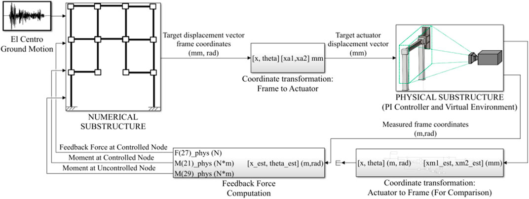
Figure 5. v-maRTHS high-level architecture in Simulink.
4 Unreal engine virtual-realistic model
4.1 Geometry creation
A virtual realistic representation of the experimental substructure is created in UE4. However, one of UE4’s limitations is its inability to create flexible objects with Euler beam like behavior directly using the UE4 interface. To overcome this challenge, SOLIDWORKS and Blender are employed to create the geometry of the 3D experimental substructure. SOLIDWORKS is used to model the built-up beam, the connector components, and the coupler. These components are then imported into UE4 as static meshes, as all these components are assumed to remain rigid through the experiment. The two S3 × 5.7 columns of the substructure are modelled in Blender as I-shaped prisms with consistent base, width, and height dimensions as listed in the benchmark problem statement. The columns are then manually meshed into eight hexahedral elements, and each element is connected to neighboring elements with “bones.” These columns are then imported into UE4 as skeletal meshes and physics assets. Adjusting the physical properties of the skeletal meshes allows the columns to appear flexible and mimic Euler beam-like deformation.
4.2 Assembling the experimental substructure
Each static mesh is assigned to its own “Static Mesh Actor.” An actor in UE4 refers to any object that can be spawned or placed into a level. Once assigned to an actor, each component is positioned and assigned material properties. Every component in the assembly is assigned UE4’s metal material. The two skeletal meshes are imported as to “Skeletal Mesh Actors.” Physics constraints between each bone of the mesh are created to represent the stiffness and damping properties of the columns while still allowing some degree of flexibility. “Physics Constraint Actors” are then used to represent contacts and boundary conditions within the model. The “Physics Constraint Actors” are also assigned the degrees of freedom, stiffness, and damping, between each component connection to represent fixed supports on the bottom of each column.
4.3 Simulink-unreal engine interface components
4.3.1 Unreal engine components
After the physical substructure is assembled, the Simulink-UE4 Interface Components (SUEICs) are added to both the Simulink and UE4 model. The components for UE4 provided freely by MathWorks, MathWorks Interface and MathWorks Automotive Content, are installed in UE4. Next, two controllable spherical actors are added to the environment to represent the hydraulic actuators. The two actuators are positioned 254 mm apart and centered on the coupler, consistent with the depiction in the benchmark problem statement. Each actuator is linked to the coupler with “Physics Constraint Actors,” and the Chaos Physics Engine is used to simulate the collisions between each component. The Chaos Physics Engine and collisions are necessary to accurately represent the actuators translating the coupler and provide key features for rigid body dynamics, such as damping and collision response. The final SUIEC added to the UE4 model is a virtual camera pointing towards the coupler. To ensure the virtual camera can accurately capture the motion in the simulation, a controlled black background and a point light are added to the environment. The recorded video data from this virtual camera is used for data collection in the computer vision-based tracking algorithm. A render of the virtual environment is shown in Figure 6.
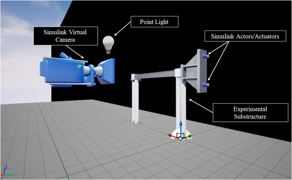
Figure 6. Virtual-realistic experimental setup in UE4.
4.3.2 Required symmetry
A major limitation of “Physics Constraint Actors” is their inability to represent a “pulling force” from the SUEIC actuators on the coupler, thus leaving the model unable to accurately simulate negative actuator displacements. To work around this issue, symmetry is introduced into the model. A second coupler is added to Node 7 of the experimental substructure and then both actuators are copied and placed behind the second coupler, as illustrated in Figure 7. In this setup the previous negative “pulling forces” are now represented as “pushing forces” on the second actuator.
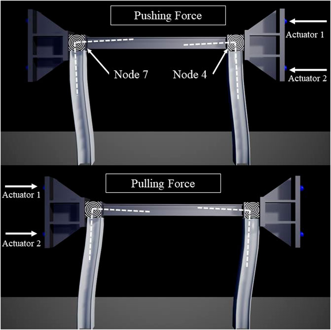
Figure 7. Depiction of the pushing and pulling couplers.
4.3.3 Simulink components
To communicate with the SUEIC actors, the Vehicle Dynamics Blockset provided by MathWorks is utilized. While the primary intent of this blockset is to simulate vehicle dynamics in various driving scenarios, it is repurposed for this project to conduct RTHS tests. The “Simulate 3D Scene Configuration” block within the blockset is used to link the virtual realistic environment to the Simulink model and allow for communication between UE4 and Simulink. Next, the “Simulation 3D Actor Transform Set” block is introduced to send the desired actuator displacement values from Simulink into the SUEIC actuators in UE4 at every time step. Likewise, the “Simulation 3D Actor Transform Get” block is used to receive measured actuator displacement values from the SUEIC actuators back to Simulink. Due to the collisions in the UE4 simulation, the actuators experience a damping effect, causing the desired and measured actuator displacements to differ, which is consistent with what one would expect in a real-world test. To be thorough, the sensor noise values are also added to each of the measured responses to preserve the representation of the force transducers. The final block used in the simulation is the “Simulation 3D Camera Get” block. This block is used to configure the mounting location and rotation, the vertical and horizontal resolution, and field of view angle of the virtual camera SUEIC setup earlier. The block then records the simulation from the specified mounting point and exports a real-time RGB array value at each time step. The combination of the virtual realistic environment in UE4 and the previously listed Simulink blocks now allow for computer vision-based tracking algorithms to be simulated in the v-maRTHS.
5 Computer vision tracking algorithm
A real-time computer vision-based tracking algorithm is used to measure the displacement of Node 4, shown previously in Figure 7 of the experimental substructure directly. The algorithm utilizes the Lucas-Kanade optical flow method to track the displacement of a specific Region of Interest (ROI) from the RGB array that is output from the simulation video at each time step (Al-Qudah and Yang, 2023). To compute the optical flow between two images, the optical flow constraint equation, Equation 1, shown below is solved.
Ω represent small spatial neighborhoods within the ROI domain, where x and y refer denote individual pixels within each spatial neighborhood. W is a window function that prioritizes the constraints towards the center of the ROI acting as the weighting factor. The solution to the weighted minimization problem is seen below in Equation 3.
The spatiotemporal derivatives
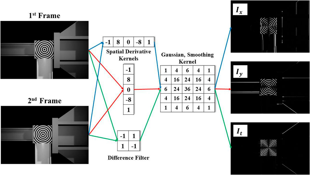
Figure 8. Lucas Kanade Optical Flow kernels.
6 Controller
6.1 MIMO controller
The controller is based on a conventional proportional-integral-derivative (PID) model, the with derivative constant omitted due to its potential to induce instability. To establish initial values for the PI controller gains, the Ziegler-Nichols closed-loop tuning method (Fahmy et al., 2014) is employed. Since the system is a MIMO system, the gains set for the control subsystem in the PID block are presented in the expression given by Equation 4:
where
The block diagram illustrated in Figure 9 depicts the experimental implementation of the control plant based on a UE4 interface aimed at achieving the most synchronized tracking possible. For this reason, the output of the control plant (measured displacements) follows the target displacement vector (numerical substructure) and evaluates the tracking, estimation and global performance of the maRTHS. Another significant aspect of this new approach is the versatility of the frame response, which is not estimated, i.e., the response of the experimental substructure provides the displacements and calculates the measured forces for the numerical substructure.
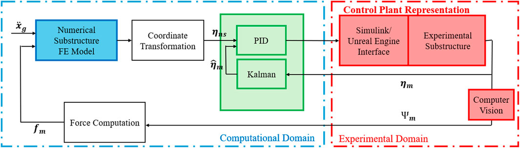
Figure 9. Computational and Experimental Domain block diagram.
In the tracking control section, one can observe the interaction scheme between the structure and the actuators. An estimate based on a Kalman filter is established for the signal filtering that acts directly on the MIMO PID controller, as previously mentioned. In this context, the displacement obtained from the actuators does not directly interfere in obtaining the measured force. This, as you can see, is obtained from the tracking algorithm for computer vision. A block diagram of the UE4 and Simulink interface is provided in Figure 10.
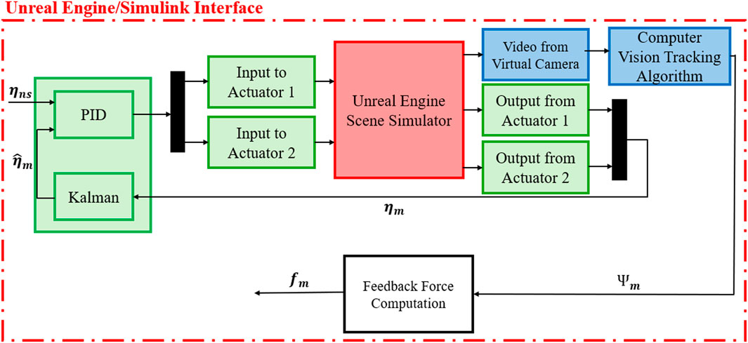
Figure 10. Unreal Engine and Simulink interface block diagram.
6.2 Kalman filter for estimating unobserved states
According to (Ziegler and Nichols, 1993), an estimator is necessary, because the measured signals,
where
In MATLAB, the Kalman function performs the estimates to minimize the steady-state error covariance. It takes the plant system and noise covariance data (Q, R and N), and returns the estimates of the output and states (Kalman: Design Kalman filter for state estimation, 2007). The process noise covariance gain, Q, and the sensor noise covariance gain, R, are positive values, which in this case are obtained from experimental measurements conducted on the multiaxial benchmark.
6.3 PID optimization
The Control Design Toolbox of MATLAB (Simulink Control Design, 2023) is an optimization package that facilitates the selection of feedback gains to meet design specifications in closed-loop control systems. The values discussed in Section 6.1 are refined through simulations or real-time testing to achieve optimal performance, selecting the optimization method, Bode, Nichols or Root Locus editor. In this case, being a MIMO system, the PI controller constants are determined for each output of the control plant, taking into account their respective responses. Using the Root Locus Editor method, the poles and zeros are strategically adjusted to determine a feasible stability range for the system that will be reflected in new gain values (Clark, 1996; Ogata, 2010). Both the open-loop frequency response and step response can be visualized simultaneously, allowing verification of proper control practice in the time-domain response—a crucial aspect of effective control design, aiming for less than 20% overshoot. This method provides a starting point for further refinement to achieve the desired control performance, balancing factors like response time, stability, and steady-state accuracy. The design methods are iterative and combine parameter selection with analysis, simulation and understanding of plant dynamics.
7 Validation of the computer vision-based tracking algorithm
7.1 Virtual camera calibration
To calibrate the virtual camera used to record the simulation, a calibration board is created to be used in the MATLAB Camera Calibrator App. The board is first modeled in SOLIDWORKS as a 200 × 200 mm square containing 50 × 50 mm checkered squares. The board is then imported into UE4 and placed 375 mm away from the virtual camera, maintaining the same distance as used in the simulation. The board is then moved side-to-side and rotated while the camera takes 9 different pictures of the process. The pictures taken of the virtual calibration board can be seen in Figure 11.

Figure 11. Nine Pictures of the calibration board at different locations and rotations.
The pictures are input into the Camera Calibrator App in MATLAB to analyze the dynamics and characteristics of the virtual camera. The app automatically recognizes the tracking points in the checkerboard and shows the errors in pixels. Images that generated larger errors are dismissed and the calibration process is repeated. Once removed, all remaining images are localized with defined positions and angles, with an overall mean error of 0.15 pixels. This process is illustrated in Figure 12.
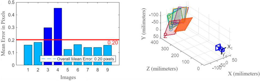
Figure 12. Error of each picture and representation of the position of the board to the camera.
The intrinsic and extrinsic camera parameters are saved in a variable containing all image information, which is recorded in Table 1. The focal length, the skew coefficient, and the first-order radial and tangential distortions are retrieved from the intrinsic parameters. Additionally, the pixel-to-mm conversion factor,
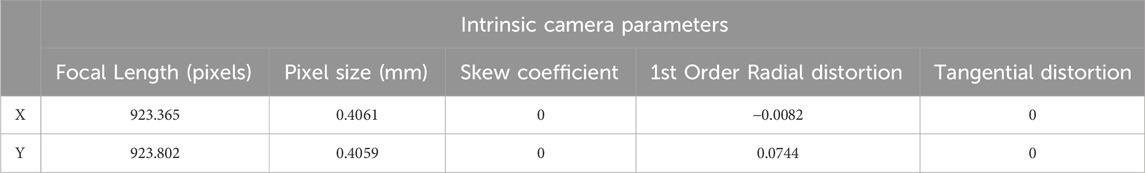
Table 1. Intrinsic Camera Parameters received from calibration.
7.2 Virtual validation experiment
The accuracy of the computer vision-based tracking algorithm is then tested in a controlled experiment. The experiment consists of a cube moving in a transverse sine wave pattern, oscillating with an amplitude of 10 mm. The noise threshold is optimized based on this experiment and implemented into the algorithm, with the results shown in Figure 13. The algorithm can track true displacement with a root mean square error of 2.02 mm without smoothing. This number drops to 0.63 mm with smoothing but due to the real time requirement and computational demands of a moving average, this was not applied in the RTHS model. The calibration experiment also suggests an inherent offset in the displacement likely due to a process that occurs in UE4 in which the model “settles” at the beginning of the simulation. The camera’s intrinsic parameters, the optimized noise threshold, and the inherent offset are implemented into the computer vision tracking algorithm to more accurately track the nodal displacement and rotation of the frame. In real time applications another cause of error is time delay. The algorithm is also optimized to reduce the time delay as much as possible. To do this, the frames are fed into the algorithm in an RGB Array format which allows for faster data processing at the expense of image detail. Another way this algorithm is optimized is using a Gaussian filter which blurs the detail of each frame but greatly reduces noise and processing time.
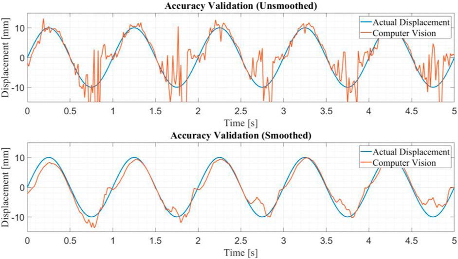
Figure 13. Results from validation experiment.
8 Experiments
Two separate experiments are conducted to compare the different experimental substructure and displacement tracking methods. The first experiment is conducted with the provided Simulink model and an optimized PID controller. The Simulink model represented the experimental substructure with a state-space model and measured the nodal displacement through transforming the actuator displacements. The second experiment is conducted using the developed virtual-realistic experimental substructure with the nodal displacement measured directly using the computer vision-based tracking algorithm, the actuator displacements are also recorded. The input for both experiments is the El Centro historic earthquake record scaled by a factor of 0.8. The error indexes are recorded and can be seen in Table 2. Comparing the tracking results of these experiments provides a means to quantitatively evaluate the performance of the MIMO PI controller while also determining the fidelity of the response of the virtual simulation compared to the analytical model. The desired nodal displacement and the rotation of the numerical substructure and the measured nodal displacement of the experimental substructure using both the computer vision-based tracking algorithm and the nonlinear coordinate transform are also recorded. By comparing the nodal displacement and rotation measurements recorded using the coordinate transform method and the computer vision tracking method, the accuracy of the computer vision tracking algorithm is quantified.
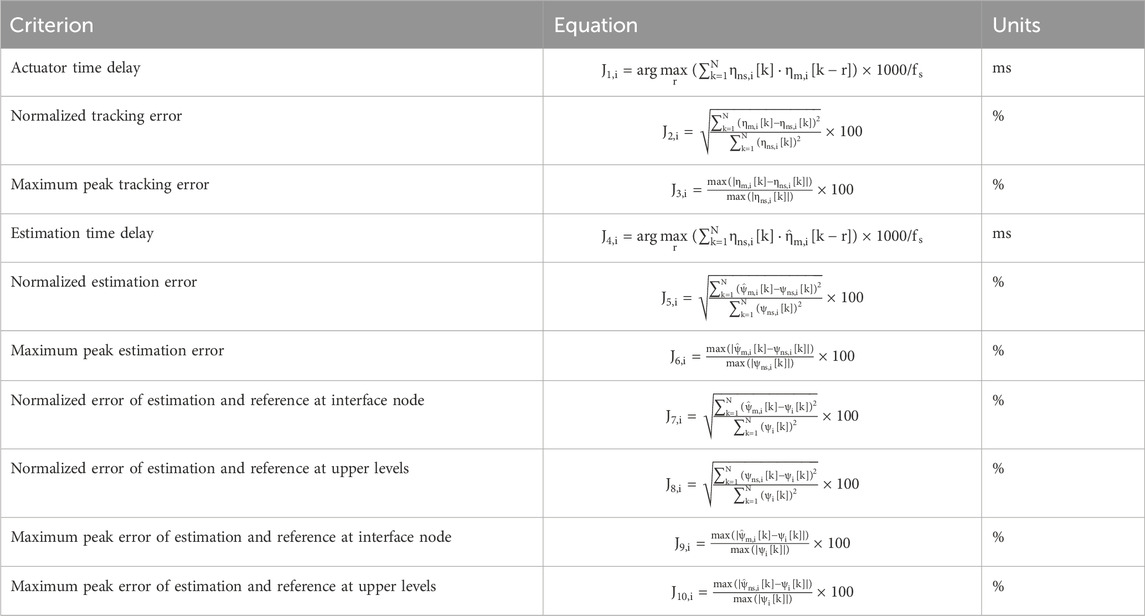
Table 2. Performance evaluation criteria.
9 Results and discussion
9.1 Evaluation of error indexes
The “Experimental Benchmark Control Problem for Multi-axial Real-time Hybrid Simulation” paper provides 10 different error indices to evaluate the performance of the controller. The formulas used to calculate each error index can be seen in Table 2.
The state-space and virtual realistic representations produce similar tracking control error index results. Using the PID controller and the provided control plant, the model can be controlled to a maximum peak tracking error under 35% and a maximum time delay of 15.63 milliseconds. Meanwhile, the virtual realistic representation can be controlled to a maximum peak tracking error of 46.63% with a maximum time delay of 19.53 milliseconds. The tracking results are plotted in Figures 14, 15.
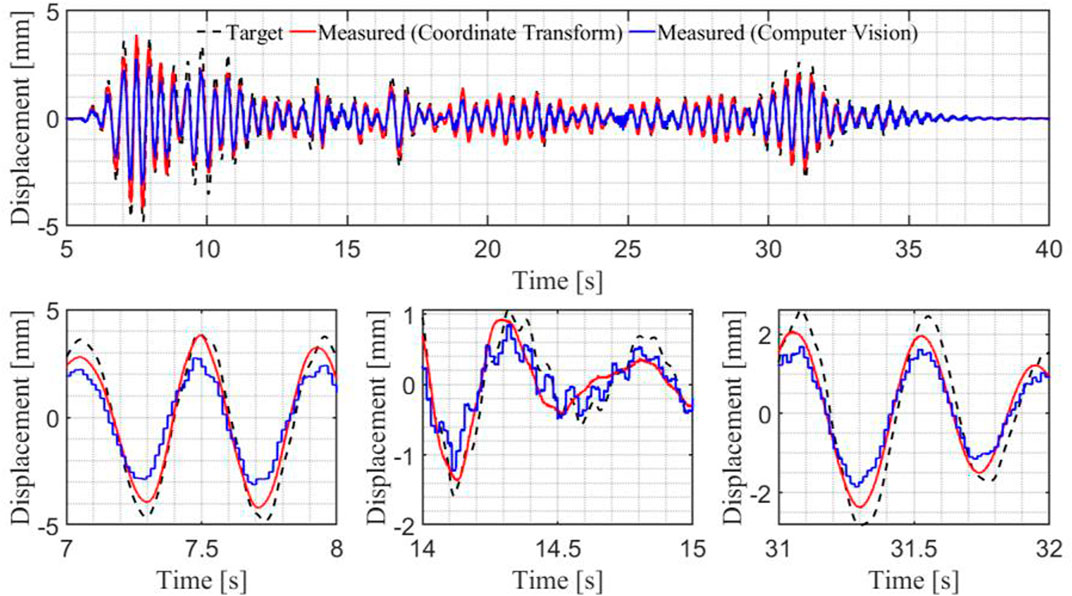
Figure 14. Comparison of the Target versus Measured actuator 1 displacements.
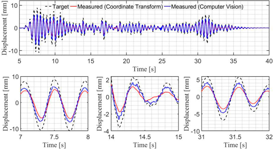
Figure 15. Comparison of the Target versus Measured actuator 2 displacements.
The estimation and global RTHS performance of the state-space representation performs significantly better than the virtual-realistic representation. The state-space model can be controlled to a maximum peak estimation error of 40.49% and a maximum peak RTHS error of 40.29%. It also records a maximum estimation time delay of 37.11 milliseconds. Meanwhile, the virtual realistic model has much higher maximum estimation and global RTHS errors of 92.5% and 94.63%, respectively. All of the error indices can be seen in Table 3. The higher estimation and global RTHS errors are due to a lack of refinement in the computer vision-based tracking algorithm and the uncertainties within the virtual realistic simulation environment. This is evident because despite similar tracking results the estimation and global errors are magnified. This is investigated in the following sections.
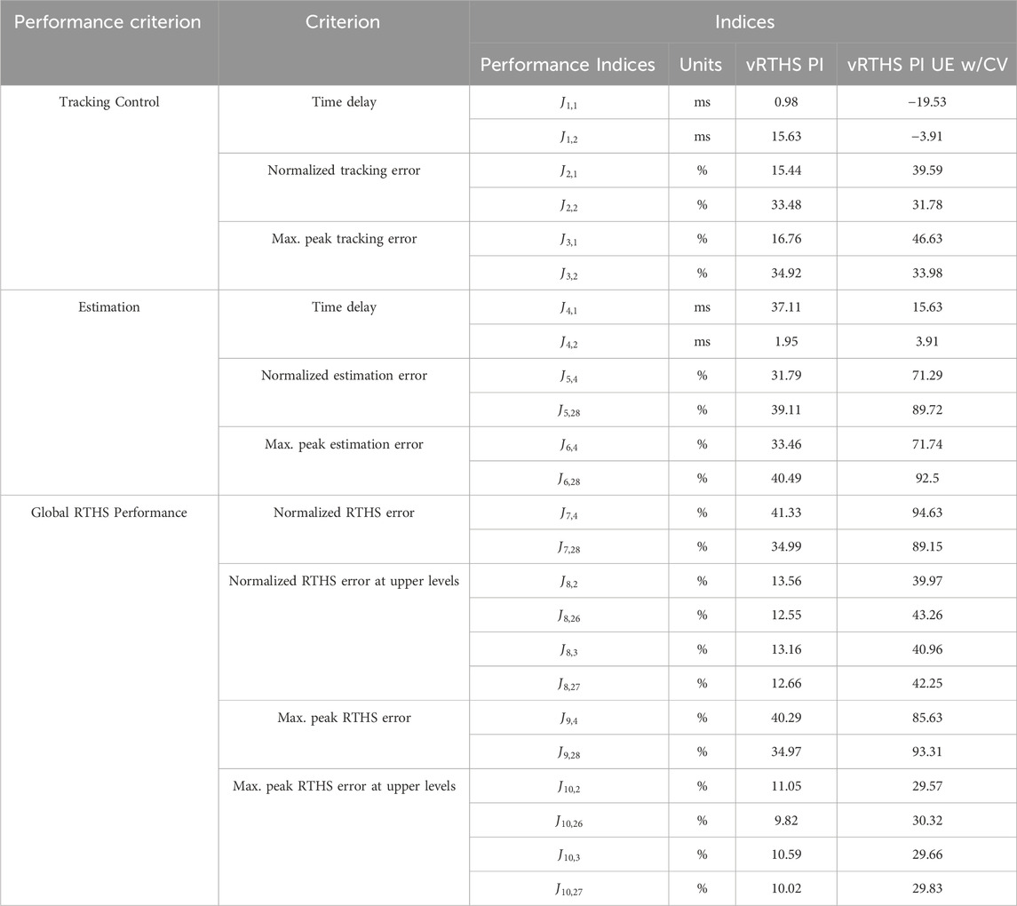
Table 3. Error indices.
9.2 Nodal tracking evaluation
The nodal tracking abilities of the nonlinear coordinate transform and the computer vision-based tracking algorithm are compared and plotted in Figure 16, below. The nonlinear coordinate transform can track the nodal displacement values within a maximum peak tracking error of 35.6% and a normalized RMSE of 0.64 using Eq. 7. The computer vision tracking algorithm can track the nodal displacement within a maximum peak tracking error of 78.8% and a normalized RMSE of 1.24. This can be seen in Figure 16.
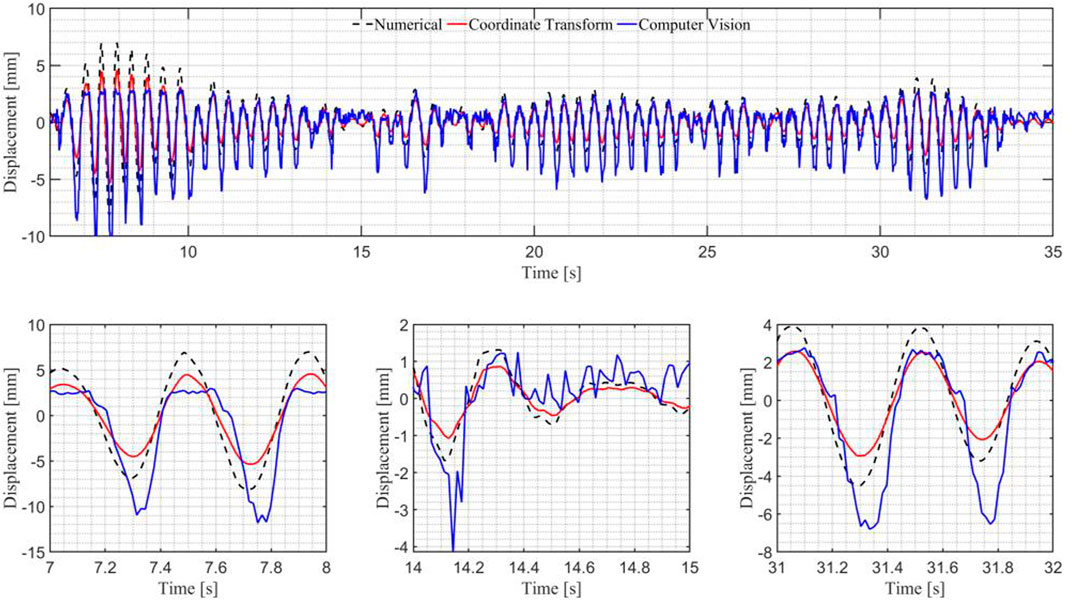
Figure 16. Nodal displacement tracking evaluation of the different tracking techniques.
The nonlinear coordinate transform is able to track the nodal rotation values within an maximum peak tracking error of 30.9% and a normalized RMSE of 0.50. The computer vision tracking algorithm was able to track the nodal displacement within a maximum peak tracking error of 70.7% and an RMS percent error of 1.10, as illustrated in Figure 17.
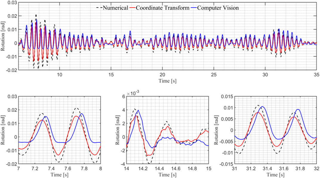
Figure 17. Nodal rotation tracking evaluation of the different tracking techniques.
9.3 Error mitigation investigation
The computer vision tracking algorithm produces higher errors when tracking the displacement and rotation of the frame, which significantly influences the estimation and global RTHS results. Additionally, noise appears to play a role in these effects, offering areas for potential improvement. As mentioned in the accuracy validation section, the addition of a moving average filter to the tracking algorithm to make it more resistant to noise can greatly improve the accuracy of the tracking results. Moving averages of different window sizes are applied to the computer vision tracking algorithm and the tracking errors are recalculated and plotted in Figure 18.
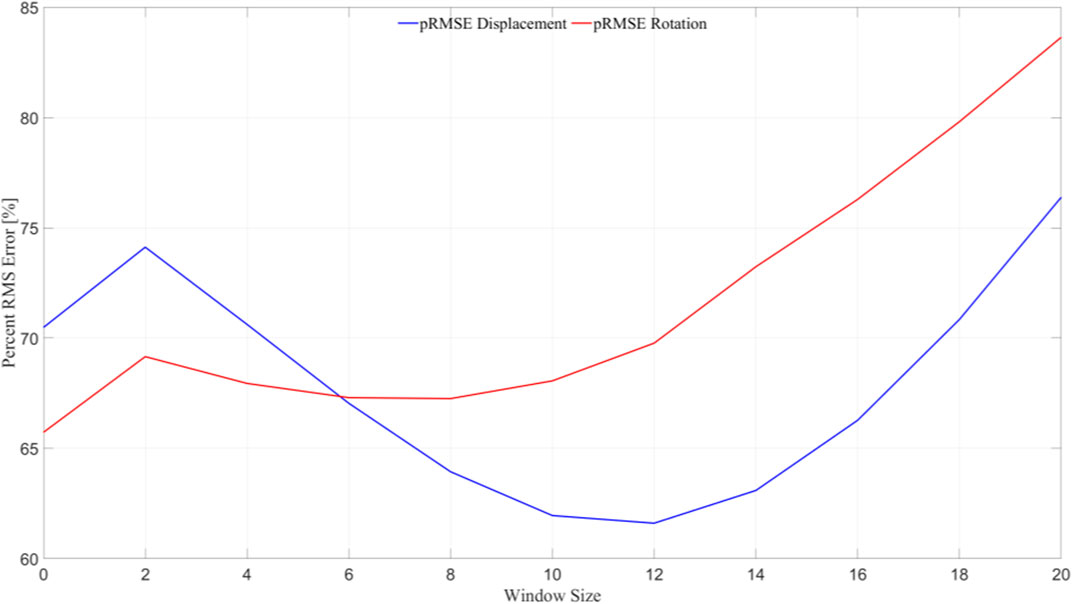
Figure 18. Error mitigation investigation.
Both the nodal displacement and rotation tracking results improve greatly when a moving average with a window size of 8 is applied to the data. The estimation and global RTHS error metrics are recalculated with this filter applied. The recalculated error indices are shown in Table 4.
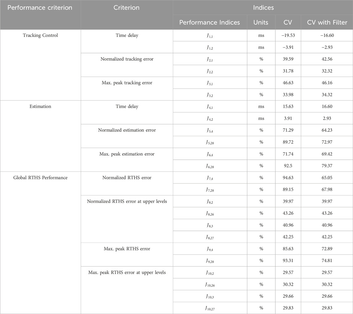
Table 4. Filter effect investigation.
The time delay errors and the RTHS errors at the upper levels are unaffected by the filter, however the remaining estimation and global RTHS indices are improved when the filter is applied. The indices that are most impacted include the normalized RTHS error at nodes 4 and 28 dropping from 94.63% to 65.05% and 89.15%–67.98%, respectively. This suggests that the algorithm will benefit greatly from a predictive moving average filter or an adaptive feedback loop to reduce the noise of the signal.
9.4 Comparison with previous PI controllers
The performance of the PI controller is compared to the tracking performance of the PI controllers that were submitted to the previous single-axis RTHS benchmark problem. This comparison quantifies the effectiveness of the PI controller implemented in this study compared to four previously successful PI controllers: the sample optimized PI controller from the previous single-axis benchmark problem, a deep reinforcement learning (DRL) PI controller, and an adaptive delay compensation PI controller. It also provides some insight into what effects multi-axial dynamics may have on PI controllers. Table 5 displays the time delay, normalized tracking error, and maximum tracking error achieved by each controller. The MIMO PI controller used in this study is separated into two columns to compare actuator tracking results independently.
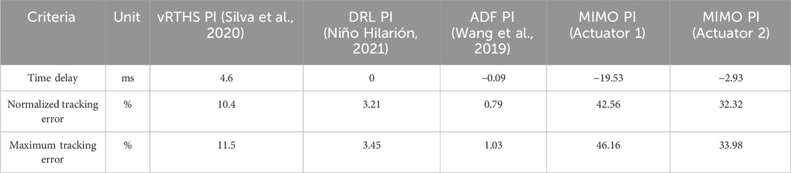
Table 5. Comparison with previous PI controllers.
The comparison of the MIMO PI controller to the initial optimized PI controller, provided with the first benchmark statement (Silva et al., 2020), suggests that the enhanced level of complexity due to multiple actuators has a great negative impact on an optimized PI controller’s performance as both controllers were made using similar methodologies. The comparison suggests that either a deep reinforcement learning feature (Niño Hilarión, 2021) or an adaptive delay feedback would greatly improve the performance of the MIMO controller.
10 Conclusion and future work
This study establishes a novel framework for applying computer vision-based tracking algorithms and sensing in v-maRTHS simulations using simulated cameras within virtual simulation environments. A computer vision displacement tracking algorithm has been developed to reduce time delays within 31.25 milliseconds while tracking the nodal displacement and rotation of the frame within a normalized RMSE of 1.24 and 1.10, respectively. Thus, demonstrating that the nodal displacement and rotation of the frame can be tracked directly using the Lucas-Kanade Optical Flow algorithm and provides an alternative method to the current method of nonlinear coordinate transformations. This study also begins to allow others to advance computer vision control theory in future v-maRTHS benchmark problems. It is shown that Unreal Engine can be a feasible approach to simulating experimental substructures of similar nature, while still being able to measure actuator imperfections and control structure interactions. The virtual simulation environment along with computer vision tracking can be interfaced with a MIMO PI controller to conduct a maRTHS with maximum actuator tracking errors of under 46.63% and 33.98% for actuators 1 and 2, respectively, and a maximum actuator time delay of 19.53 milliseconds and 3.91 milliseconds.
With these conclusions, there are areas that could be further explored. Firstly, this experiment could be simulated with an event-based imager. An event-based imager has a much higher sampling frequency than a traditional camera and can be a viable option to record higher frequency tests in the laboratory, producing shorter time delays and higher tracking accuracy. Secondly, increasing the model fidelity of the virtual-realistic model, including using a more detailed mesh, and more accurate contact points, could enhance the realism of the simulation. Lastly, applying a computer-vision controller or a more sophisticated PI controller into the model could yield better tracking results.
Data availability statement
The raw data supporting the conclusions of this article will be made available by the authors, without undue reservation.
Author contributions
WS: Conceptualization, Data curation, Formal Analysis, Investigation, Methodology, Project administration, Software, Validation, Visualization, Writing–original draft. PM: Conceptualization, Formal Analysis, Investigation, Methodology, Software, Validation, Visualization, Writing–original draft. GT: Conceptualization, Formal Analysis, Methodology, Software, Visualization, Writing–original draft. CS: Conceptualization, Formal Analysis, Methodology, Software, Supervision, Writing–original draft, Writing–review and editing. AO: Conceptualization, Formal Analysis, Investigation, Methodology, Project administration, Supervision, Writing–original draft, Writing–review and editing. FM: Conceptualization, Funding acquisition, Project administration, Resources, Supervision, Writing–review and editing.
Funding
The author(s) declare that financial support was received for the research, authorship, and/or publication of this article. The authors appreciate the support of NSF Division of Information and Intelligent Systems (IIS) CISE, Hardening the Data Revolution DSC, Grant/Award Number: 2123346; and Office of Naval Research, research program: Structural Reliability, ONR 331, Grant No: 13620990, Award Number: N00014-22-1-2638.
Acknowledgments
The authors thank the creators of the “Experimental Benchmark Control Problem for Multi-axial Real-time Hybrid Simulation” for the opportunity to compete in this competition and for driving this research objective. The authors would like to thank the UNM Center for Advanced Research Computing, supported in part by the National Science Foundation, for providing the laboratory space and office resources used to conduct this work. The authors also thank Brandon Sisk and Duncan Gardener for their early assistance with this research.
Conflict of interest
The authors declare that the research was conducted in the absence of any commercial or financial relationships that could be construed as a potential conflict of interest.
Publisher’s note
All claims expressed in this article are solely those of the authors and do not necessarily represent those of their affiliated organizations, or those of the publisher, the editors and the reviewers. Any product that may be evaluated in this article, or claim that may be made by its manufacturer, is not guaranteed or endorsed by the publisher.
References
Aguila, A. J., Li, H., Palacio-Betancur, A., Ahmed, K. A., Kovalenko, I., and Gutierrez Soto, M. (2024). Conditional adaptive time series compensation and control design for multi-axial real-time hybrid simulation. Front. Built Environ. 10, 1384235. doi:10.3389/fbuil.2024.1384235
Ahmine, Y., Caron, G., Mouaddib, El M., and Chouireb, F. (2019). Adaptive lucas-kanade tracking. Image Vis. Comput. 88, 1–8. 0262-8856. doi:10.1016/j.imavis.2019.04.004
Ali, K., Yuan, X., Davtalab, O., and Khoshnevis, B. (2019). Computer vision for real-time extrusion quality monitoring and control in robotic construction. Automation Constr. 101, 92–98. doi:10.1016/j.autcon.2019.01.022
Al-Qudah, S., and Yang, M. (2023). Large displacement detection using improved lucas–kanade optical flow. Sensors 23, 3152. doi:10.3390/s23063152
Aminfar, A. H., Davoodzadeh, N., Aguilar, G., and Princevac, M. (2019). Application of optical flow algorithms to laser speckle imaging. Microvasc. Res. 122, 52–59. ISSN 0026-2862. doi:10.1016/j.mvr.2018.11.001
Barron, J. L., Fleet, D. J., Beauchemin, S. S., and Burkitt, T. A. (1992). “Performance of optical flow techniques,” in Proceedings of the IEEE Conference on Computer Vision and Pattern Recognition (CVPR), Champaign, IL: CVPR, 236–242.
Carrion, J. E., and Spencer, B. F. (2007). Model-based strategies for real-time hybrid testing. University of Illinois at Urbana-Champaign.
Condori, J. W., Salmeron, M., Patino, E., Montoya, H., Dyke, S. J., Silva, C. E., et al. (2023). Experimental benchmark control problem for multi-axial real-time hybrid simulation. Front. Built Environ. 9. doi:10.3389/fbuil.2023.1270996
Dan, L., Dai-Hong, J., Rong, B., Jin-Ping, S., Wen-Jing, Z., and Chao, W. (2017). “Moving object tracking method based on improved lucas-kanade sparse optical flow algorithm,” in 2017 International Smart Cities Conference (ISC2), Wuxi, China, 14-17 September 2017, 1–5.
Davis, A., et al. (2024). “Digital twins for photorealistic event-based structural dynamics,” in Computer vision and laser vibrometry, volume 6. SEM 2023. Conference proceedings of the society for experimental Mechanics series. Editors J. Baqersad, and D. Di Maio (Cham: Springer). doi:10.1007/978-3-031-34910-2_13
Dyke, S. J., Spencer, B. F., Quast, P., and Sain, M. (1995). Role of control-structure interaction in protective system design. J. Eng. Mech. 121, 322–338. doi:10.1061/(asce)0733-9399(1995)121:2(322)
Fahmy, R., Badr, R., and Rah, F. (2014). Adaptive PID controller using RLS for SISO stable and unstable systems. Adv. Power Electron., 5. doi:10.1155/2014/507142
Fermandois, G. A. (2019). Application of model-based compensation methods to real-time hybrid simulation benchmark. Mech. Syst. Signal Process. 131, 394–416. 0888-3270. doi:10.1016/j.ymssp.2019.05.041
Ferrero, R., Gandino, F., Hemmatpour, M., Montrucchio, B., and Rebaudengo, M. “Exploiting accelerometers to estimate displacement,” in 2016 5th Mediterranean Conference on Embedded Computing (MECO), Bar, Montenegro, Bar, Montenegro, 12-16 June 2016, 206–210. keywords: {Accelerometers;Acceleration;Kalman filters;Estimation;Noise measurement;Motion measurement;Frequency measurement;accelerometer;Kalman filter;position tracking;displacement}.
Guo, J., and Zhu, C. (2016). Dynamic displacement measurement of large-scale structures based on the Lucas–Kanade template tracking algorithm. Mech. Syst. Signal Process. 66–67, 425–436. ISSN 0888-3270. doi:10.1016/j.ymssp.2015.06.004
Hakuno, M., Shidawara, M., and Hara, T. (1969). Dynamic destructive test of a cantilever beam, controlled by an analog-computer. Proc. Jpn. Soc. Civ. Eng. 1969, 1–9. doi:10.2208/jscej1969.1969.171_1
Horiuchi, T., Inoue, M., Konno, T., and Namita, T. (1999). Real-time hybrid experimental system with actuator delay compensation and its application to a piping system with energy absorber. Earthq. Eng. Struct. Dyn. 28, 1121–1141. doi:10.1002/(sici)1096-9845(199910)28:10<1121::aid-eqe858>3.3.co;2-f
Kalman: Design Kalman filter for state estimation (2007). MathWorks. Available at: https://la.mathworks.com/help/control/ref/ss.kalman.html?lang=en.
Li, H., Amin, M., Montoya, H., Uribe, J. W. C., Dyke, S. J., and Xu, Z. (2021). Sliding mode control design for the benchmark problem in real-time hybrid simulation. Mech. Syst. Signal Process. 151, 107364. doi:10.1016/j.ymssp.2020.107364
Liu, X., Li, Q., Wang, L., Lin, M., and Wu, J. (2023). Data-Driven state of charge estimation for power battery with improved extended kalman filter. IEEE Trans. Instrum. Meas. 72, 1–10. keywords: {State of charge;Estimation;Batteries;Neural networks;Kalman filters;Mathematical models;Integrated circuit modeling;Back-propagation (BP) neural network;extended Kalman filter (EKF);lithium-ion battery;state of charge (SOC);variance compensation}. doi:10.1109/TIM.2023.3239629
Manigel, J., and Leonhard, W. (1992). Vehicle control by computer vision. IEEE Trans. Industrial Electron. 39 (3), 181–188. keywords: {Computer vision;Remotely operated vehicles;Road vehicles;Computer displays;Mobile robots;Guidelines;Charge coupled devices;Charge-coupled image sensors;Cameras;Automotive components}. doi:10.1109/41.141618
Nakata, N., Dyke, S., Zhang, J., Mosqueda, G., Shao, X., Mahmoud, H., et al. (2014). Hybrid simulation primer and dictionary. Available at: https://datacenterhub.org/resources/8102.
Niño Hilarión, A. (2021). Using deep reinforcement learning to design a tracking controller for a real-time hybrid simulation benchmark problem. Univ. los Andes. Dispon. Available at: http://hdl.handle.net/1992/55345.
Ou, Ge, Ozdagli, A. I., Dyke, S. J., and Wu, B. (2015). Robust integrated actuator control: experimental verification and real-time hybrid-simulation implementation. Earthq. Eng. Struct. Dyn. 44, 441–460. doi:10.1002/eqe.2479
Palacio-Betancur, A., and Gutierrez Soto, M. (2022). Recent advances in computational methodologies for real-time hybrid simulation of engineering structures. Archives of Computational Methods in Engineering.
Shao, X., Reinhorn, A. M., and Sivaselvan, M. V. (2011). Real-time hybrid simulation using shake tables and dynamic actuators. J. Struct. Eng. 137 (7), 748–760. doi:10.1061/(ASCE)ST.1943-541X.0000314
Silva, C. E., Gomez, D., Maghareh, A., Dyke, S. J., and Spencer, B. F. (2020). Benchmark control problem for real-time hybrid simulation. Mech. Syst. Signal Process. 135, 106381. doi:10.1016/j.ymssp.2019.106381
Simulink Control Design (2023). MathWorks," MathWorks. Available at: https://la.mathworks.com/help/control/ref/controlsystemdesigner-app.html.
Takanashi, K., Udagawa, K., Seki, M., Okada, T., and Tanaka, H. (1975). Nonlinear earthquake response analysis of structures by a computer-actuator on-line system. Earthquake Resistant Structure Research Center.
Tao, J., and Mercan, O. (2019). A study on a benchmark control problem for real-time hybrid simulation with a tracking error-based adaptive compensator combined with a supplementary proportional-integral-derivative controller. Mech. Syst. Signal Process. 134, 106346. 0888-3270. doi:10.1016/j.ymssp.2019.106346
Wang, Z., Ning, X., Xu, G., Zhou, H., and Wu, B. (2019). High performance compensation using an adaptive strategy for real-time hybrid simulation. Mech. Syst. Signal Process. 133, 106262. ISSN 0888-3270. doi:10.1016/j.ymssp.2019.106262
Xu, W., Meng, X., Chen, C., Guo, T., and Peng, C. (2024). Evaluation of data-driven-narx model-based compensation for multi-axial real-time hybrid simulation benchmark study. Front. Built Environ. 10, 1374819. doi:10.3389/fbuil.2024.1374819
Ziegler, J. G., and Nichols, N. B. (1993). Optimum settings for automatic controllers. J. Dyn. Syst. Meas. Control-transactions Asme 115, 220–222. doi:10.1115/1.2899060
Keywords: real-time hybrid simulation, computer vision, multi-axial test, virtual reality, control
Citation: Saeger W, Miranda P, Toledo G, Silva CE, Ozdagli A and Moreu F (2024) A framework for computer vision for virtual-realistic multi-axial real-time hybrid simulation. Front. Built Environ. 10:1415032. doi: 10.3389/fbuil.2024.1415032
Received: 09 April 2024; Accepted: 22 July 2024;
Published: 08 August 2024.
Edited by:
Tao Wang, China Earthquake Administration, ChinaReviewed by:
Wael A. Altabey, Alexandria University, EgyptChia-Ming Chang, National Taiwan University, Taiwan
Copyright © 2024 Saeger, Miranda, Toledo, Silva, Ozdagli and Moreu. This is an open-access article distributed under the terms of the Creative Commons Attribution License (CC BY). The use, distribution or reproduction in other forums is permitted, provided the original author(s) and the copyright owner(s) are credited and that the original publication in this journal is cited, in accordance with accepted academic practice. No use, distribution or reproduction is permitted which does not comply with these terms.
*Correspondence: F. Moreu, Zm1vcmV1QHVubS5lZHU=