Predicting the impact of adding metakaolin on the splitting strength of concrete using ensemble ML classification and symbolic regression techniques –a comparative study

The mechanical characteristics of concrete are crucial factors in structural design standards especially in concrete technology. Employing reliable prediction models for concrete’s mechanical properties can reduce the number of necessary laboratory trials, checks and experiments to obtain valuable representative design data, thus saving both time and resources. Metakaolin (MK) is commonly utilized as a supplementary replacement for Portland cement in sustainable concrete production due to its technical and environmental benefits towards net-zero goals of the United Nations Sustainable Development Goals (UNSDGs). In this research work, 204 data entries from concrete mixes produced with the addition of metakaolin (MK) were collected and analyzed using eight (8) ensemble machine learning tools and one (1) symbolic regression technique. The application of multiple machine learning protocols such as the ensemble group and the symbolic regression techniques have not been presented in any previous research work on the modeling of splitting tensile strength of MK mixed concrete. The data was partitioned and applied according to standard conditions. Lastly, some selected performance evaluation indices were used to test the models’ accuracy in predicting the splitting strength (Fsp) of the studied MK-mixed concrete. At the end, results show that the k-nearest neighbor (KNN) outperformed the other techniques in the ensemble group with the following indices; SSE of 4% and 1%, MAE of 0.1 and 0.2 MPa, MSE of 0, RMSE of 0.1 and 0.2 MPa, Error of 0.04% and 0.04%, Accuracy of 0.96 and 0.96 and R2 of 0.98 and 0.98 for the training and validation models, respectively. This is followed closely by the support vector machine (SVM) with the following indices; SSE of 7% and 3%, MAE of 0.2 and 0.2 MPa, MSE of 0.0 and 0.1 MPa, RMSE of 0.2 and 0.3 MPa, Error of 0.05% and 0.06%, Accuracy of 0.95 and 0.94, and R2 of 0.96 and 0.95, for the training and validation models, respectively. The third model in the superiority rank is the CN2 with the following performance indices; SSE of 15% and 4%, MAE of 0.2 and 0.2 MPa, MSE of 0.1 and 0.1 MPa, RMSE of 0.3 and 0.3 MPa, Error of 0.08% and 0.07%, Accuracy of 0.92 and 0.93 and R2 of 0.92 and 0.93, for the training and validation models, respectively. These models outperformed the models utilized on the MK-mixed concrete found in the literature, therefore are the better decisive modes for the prediction of the splitting strength (Fsp) of the studied MK-mixed concrete with 204 mix data entries. Conversely, the NB and SGD produced unacceptable model performances, however, this is true for the modeled database collected for the MK-mixed Fsp. The RSM model also produced superior performance with an accuracy of over 95% and adequate precision of more than 27. Overall, the KNN, SVM, CN2 and RSM have shown to possess the potential to predict the MK-mixed Fsp for structural concrete designs and production.

1 Introduction

The splitting tensile strength of concrete, also known as the splitting strength, is a measure of the tensile strength of concrete perpendicular to the direction of the applied load (Shah et al., 2022a). It is an important mechanical property of concrete, particularly in applications where the concrete is subjected to tensile stresses, such as in reinforced concrete beams or slabs (Ray et al., 2023). To determine the splitting tensile strength of concrete, a cylindrical or prismatic specimen is typically tested (Shah et al., 2022b). The specimen is subjected to a compressive load along its longitudinal axis while diametral tensile stresses are induced perpendicular to the applied load (Ray et al., 2021). This test is commonly referred to as the “Brazilian test” or “indirect tensile test.” During the test, the concrete specimen undergoes tensile failure along a plane perpendicular to the applied load, resulting in a tensile crack that propagates across the diameter of the specimen (Kannan and Ganesan, 2014). The splitting tensile strength is calculated by dividing the maximum tensile load applied to the specimen by the cross-sectional area perpendicular to the applied load (Guneyisi et al., 2008).The splitting tensile strength of concrete is influenced by various factors, including the composition of the concrete mix (such as the type and proportion of aggregates, cementitious materials, and admixtures), the curing conditions, the age of the concrete at testing, and the size and shape of the specimen (Khan and Haq, 2020). Generally, the splitting tensile strength of concrete is lower than its compressive strength, but it still provides valuable information about the concrete’s behavior under tensile loading conditions (Dinakar et al., 2013). Engineers use the splitting tensile strength of concrete in structural design to assess the cracking potential and durability of concrete elements subjected to tensile stresses (Ray et al., 2023). It is also used in quality control and quality assurance procedures to ensure that concrete mixes meet the required strength specifications for specific applications (Kannan and Ganesan, 2014).

The addition of metakaolin to concrete can have a significant impact on its splitting tensile strength. Metakaolin, as a pozzolanic mineral admixture, reacts with calcium hydroxide (lime) in the presence of water to form additional calcium silicate hydrate (C-S-H) gel (Guneyisi et al., 2008). This reaction contributes to the densification of the concrete matrix and improves its mechanical properties, including splitting tensile strength (Al-alaily and Hassan, 2016). Here are some key impacts of metakaolin on the splitting strength of concrete: Enhanced Microstructure: Metakaolin contributes to the refinement of the pore structure in concrete, leading to a denser and more homogeneous microstructure (Onyelowe K. C. et al., 2022). This improvement in microstructure enhances the interfacial bond between the cementitious matrix and aggregates, resulting in increased resistance to tensile stresses and improved splitting tensile strength (Onyelowe et al., 2022b). The pozzolanic reaction between metakaolin and lime leads to the formation of additional C-S-H gel, which contributes to increased strength and cohesion within the concrete matrix (Onyelowe KC. et al., 2022). As a result, concrete containing metakaolin typically exhibits higher splitting tensile strength compared to plain concrete without metakaolin (Onyelowe et al., 2022d). The incorporation of metakaolin into concrete can lead to a reduction in pore size and porosity. This reduction in porosity improves the concrete’s resistance to tensile cracking and enhances its splitting tensile strength (Shah et al., 2022a; Onyelowe et al., 2022e). Metakaolin can improve the durability of concrete by reducing permeability and increasing resistance to chemical attack and freeze-thaw cycles (Onyelowe et al., 2023a). These improvements in durability can contribute to the long-term performance and strength retention of concrete elements subjected to tensile stresses (Onyelowe et al., 2023c). Overall, the addition of metakaolin to concrete can result in concrete with enhanced splitting tensile strength, improved microstructure, and increased durability (Onyelowe and Ebid, 2023). However, the extent of improvement in splitting tensile strength may vary depending on factors such as the dosage of metakaolin, the quality of other concrete ingredients, curing conditions, and the specific characteristics of the aggregate and cementitious materials used (Dinakar et al., 2013). Optimal dosage levels and mix proportions should be carefully evaluated through laboratory testing and trial mixes to achieve the desired enhancement in splitting tensile strength while maintaining other performance criteria. The present research flowchart is presented in Figure 1, which illustrates the main focus of this present research project.

Figure 1

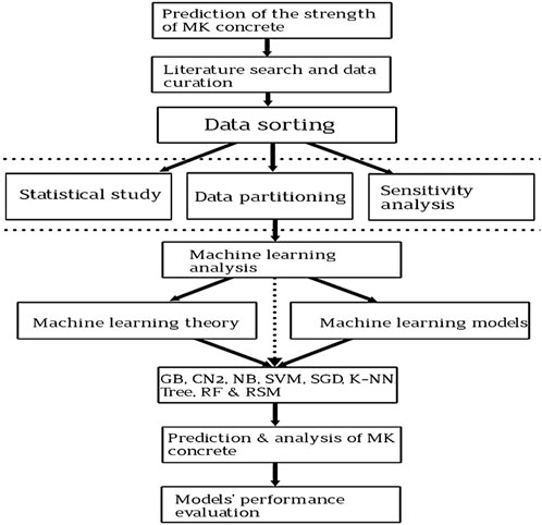
Figure 1. Flowchart of research.

2 Literature reviews

Shah et al. (2022a) used the M5P model tree algorithm to forecast the compressive strength (CS) and splitting tensile strength (STS) of concrete that includes silica fume (SF). Extensive databases were generated, and the models were evaluated using statistical metrics and parametric analysis. The trained models provide a fast and precise tool for designers to efficiently determine the appropriate proportions of silica fume concrete, resulting in time and cost savings compared to conducting laboratory trials and tests. Ray et al. (2023) forecasted the compressive and splitting tensile strength of concrete produced with waste Coarse Ceramic aggregate (CCA) and Nylon Fibre by employing machine learning techniques, specifically Support Vector Machine (SVM) and Gradient Boosting Machine (GBM). The models were trained using a comprehensive dataset consisting of 162 test results obtained from nine different mix proportions. The findings indicated that GBM had superior performance compared to SVM in terms of coefficient of determination and statistical accuracy, particularly in predicting the mechanical strength of concrete. Shah et al. (2022b) developed models that accurately predict the mechanical properties of concrete containing metakaolin (MK) using four different machine learning techniques: gene expression programming (GEP), artificial neural network (ANN), M5P model tree method, and random forest (RF). The study collected data from peer-reviewed documents and determined that RF exhibits superior predictive and generalization capabilities compared to GEP, ANN, and M5P model tree method. The study additionally discovered that the optimal ratios of MK as a partial substitute for cement are 10% for FS and 15% for both. Also, Ray et al. (2021) examined the utilization of ceramic waste as a substitute for natural aggregate in concrete. It assessed engineering characteristics such as bulk density, water absorption, and workability. An SVM-based prediction model is presented for forecasting compressive and splitting tensile strength. The model demonstrated a high accuracy level over 90%, as determined by the coefficient of determination (R²). It effectively predicted the strength of concrete with varying quantities of ceramic material. Kannan and Ganesan (2014) assessed the mechanical characteristics of self-compacting concrete (SCC) using combinations of metakaolin and fly ash (FA) in binary and ternary cementitious mixes. The investigation revealed that augmenting the proportion of MK, FA, and MK+FA had a substantial positive impact on the mechanical characteristics of SCC. The ternary mixture of cement with 15% metakaolin and 15% fly exhibited superior workability and mechanical qualities compared to the standard self-consolidating concrete (SCC) sample without MK or FA. Güneyisi et al. (2008) investigated the utilization of metakaolin (MK) as an additional cementitious ingredient to improve the performance of concrete. The process employs two alternative MK substitution rates: 10% and 20% based on the weight of Portland cement. The findings indicated that MK diminishes drying shrinkage strain while enhancing concrete strengths. The extent of these effects is contingent upon the replacement level, water-to-cement ratio, and testing age. At a 20% replacement rate, Ultrafine MK improves the pore structure of concrete and increases its impermeability. Another, Khan et al. (2020) investigated the extended-term robustness and resilience of concrete blends incorporating rice husk ash (RHA), metakaolin, and silica fume (SF) as alternatives to cement content. Workability, compressive strength, splitting tensile strength, and water absorption were evaluated for seven different types of mixtures. The findings indicated that the use of supplementary cementitious materials (SCMs) leads to a reduction in the strength of the matrix during the initial 28 days of curing. However, they thereafter contribute to the restoration of strength. A multivariable non-linear regression model was suggested to estimate the compression strength, tension strengths, and water absorption capacity. Dinakar et al. (2013) investigated the influence of metakaolin (MK) on the mechanical and durability characteristics of high strength concrete. This study determined that a substitution level of 10% of MK yielded the highest compressive strength, reaching a maximum value of 106 MPa. The strong resistance exhibited by MK concretes suggested that local MK has the capability to produce concretes with superior performance. Al-alaily et al. (2016) enhanced the strength and reduce the chloride permeability of concrete by using metakaolin (MK). The study conducted an experiment on 53 different concrete mixtures using the improved response surface method. The experiment took into account several aspects such as the total amount of binder, the percentage of MK (a specific type of binder), and the ratio of water to binder. The findings demonstrated the utility of the proposed models and design charts in comprehending crucial variables and forecasting the most advantageous mixture proportions for certain applications. It is important to note that this present work has reported the application of multiple machine learning techniques comprising of the ensemble and symbolic regression groups, which present nine different techniques. It is significant that future research project focusing on recent developments in machine learning application in civil engineering will refer to this article. It also gives MK mixed concrete designer opportunities to select the best models out of nine to forecast the concrete optimal splitting tensile strength.

3 Methodology

3.1 Data collection, sorting and preliminary statistics

After an extensive literature search, a globally representative database of two hundred and four (204) records were collected from literature (Shah et al., 2022a; 2022b) for splitting strength for different mixing ratios of meta-kaolin with concrete at different ages. The previous studies had applied the ANN, M5P, and the RF to predict the mechanical properties of the studied concrete but the present research paper reports the application of multiple machine learning techniques. Each record contains the following data: C-the content of cement (kg/m³), MK-the content of meta-kaolin (kg/m³), W-the content of water (kg/m³) or (litre/m³), FAg-the content of fine aggregates (kg/m³), CAg-the content of coarse aggregates (kg/m³), P-the content of super-plasticizer (kg/m³), Age-the concrete age at testing (days), and Fsp-Splitting tensile strength (MPa). The collected records were divided into training set (164 records≈80%) and validation set (40 records≈ 20%). Table 1 summarizes their statistical characteristics. Finally, Figure 2 shows the Pearson correlation matrix, histograms, and the relations between variables.

Table 1

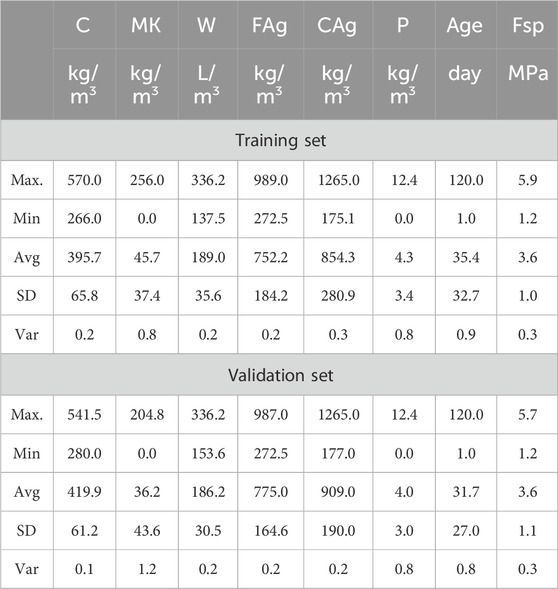
Table 1. Statistical analysis of collected database.

Figure 2

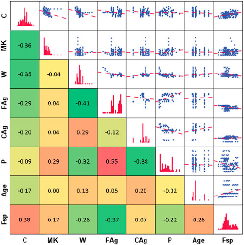
Figure 2. Correlation, distribution and interpreting chart.

3.2 Sensitivity analysis

A preliminary sensitivity analysis was carried out on the collected database to estimate the impact of each input on the (Y) values. “Single variable per time” technique is used to determine the “Sensitivity Index” (SI) for each input using the Hoffman and Gardener (1983) and Handy (1994) formula in Eq. 1 as follows:

$SI\left(X_n\right)=\frac{Y\left(X_{\mathit{max}}\right)-Y\left(X_{\mathit{min}}\right)}{Y\left(X_{\mathit{max}}\right)}(1)$

A sensitivity index of 1.0 indicates complete sensitivity, a sensitivity index less than 0.01 indicates that the model is insensitive to changes in the parameter. Figure 3 shows the sensitivity analysis with respect to Fsp.

Figure 3

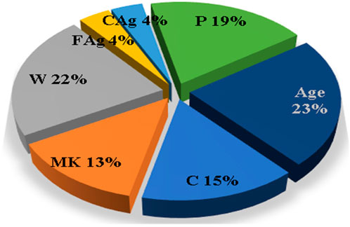
Figure 3. Sensitivity analysis with respect to Fsp.

3.3 Research program

Eight different ensemble ML classification techniques and one symbolic regression technique were used to predict the splitting tensile strength of concrete mixed with meta-kaolin using the collected database. These techniques are “Gradient Boosting (GB),” “CN2 Rule Induction (CN2),” “Naive Bayes (NB),” “Support vector machine (SVM),” “Stochastic Gradient Descent (SGD),” “K-Nearest Neighbors (KNN),” “Tree Decision (Tree)” and “Random Forest (RF)” and the “Response Surface Methodology (RSM).” The developed models were used to predict (Fsp) using the concrete mixture component contents (C, MK, W, FAg, CAg, P) and the concrete age (Age). All the developed ensemble models were created using “Orange Data Mining” software version 3.36. The considered data flow diagram is Supplementary Material.

3.4 Theory of the ML techniques

3.4.1 Gradient boosting (GB)

Gradient Boosting is a powerful ensemble learning technique used for both regression and classification tasks (Ebid, 2020). The theoretical framework is provided in Supplementary Material. Here are some advantages of Gradient Boosting over other machine learning techniques: High Predictive Accuracy: Gradient Boosting typically achieves high predictive accuracy compared to other machine learning algorithms. By combining the predictions of multiple weak learners (typically decision trees), it can capture complex relationships in the data and achieve strong generalization performance (Onyelowe et al., 2023b). Handles Non-linearity and Interactions: Gradient Boosting can capture non-linear relationships and interactions between features in the data. It does so by sequentially fitting new models to the residuals of the previous models, effectively reducing the bias and variance of the ensemble (Ebid, 2020). Robustness to Overfitting: Gradient Boosting is less prone to overfitting than individual decision trees, especially when using techniques such as regularization (e.g., shrinkage) and early stopping. These techniques help prevent the model from memorizing noise in the training data and improve its ability to generalize to unseen data (Onyelowe et al., 2023b). Gradient Boosting provides an estimate of feature importance, indicating which features are most influential in making predictions. This information can help identify the most relevant features for prediction and provide insights into the underlying data patterns (Ebid, 2020). Gradient Boosting can handle missing values in the data without the need for imputation techniques. It can learn to make predictions using the available information in the dataset, even when certain features have missing values (Onyelowe et al., 2023b). Gradient Boosting can be applied to a wide range of machine learning tasks, including regression, classification, and ranking. It supports various loss functions and can be customized by adjusting hyperparameters such as the learning rate, tree depth, and number of trees. Gradient Boosting algorithms can be parallelized, allowing for efficient distributed computing across multiple processors or computing nodes. This makes it suitable for training large-scale models on clusters or cloud computing platforms. Overall, Gradient Boosting is a versatile and effective algorithm that performs well in a variety of machine learning tasks. Its ability to handle complex data patterns, robustness to overfitting, and interpretability make it a popular choice among data scientists and machine learning practitioners. Hyperparameter tuning is crucial for optimizing the performance of Gradient Boosting models. Here are some key hyperparameters to consider tuning for Gradient Boosting: Number of Trees (n_estimators): This parameter controls the number of boosting stages (trees) to be built. Increasing the number of trees may improve model performance, but it also increases the risk of overfitting and training time. Learning Rate (learning_rate): The learning rate controls the contribution of each tree to the final ensemble. Lower learning rates require more trees to achieve similar performance but can improve generalization. It is essential to tune this parameter along with the number of trees to find the right balance between model complexity and generalization. Tree Depth (max_depth): This parameter specifies the maximum depth of each tree in the ensemble. Deeper trees can capture more complex relationships in the data but may also lead to overfitting. It is crucial to tune this parameter to prevent overfitting and improve model generalization. Minimum Samples Split (min_samples_split): This parameter specifies the minimum number of samples required to split an internal node. Increasing this parameter can help prevent overfitting by imposing a constraint on the tree’s growth. Minimum Samples Leaf (min_samples_leaf): This parameter specifies the minimum number of samples required to be at a leaf node. Increasing this parameter can help prevent overfitting and improve the robustness of the model to noise in the data. Maximum Features (max_features): This parameter controls the number of features to consider when searching for the best split at each node. It can help reduce overfitting and improve model generalization by limiting the number of features considered. Subsample Ratio (subsample): This parameter specifies the fraction of samples to be used for fitting each tree. It can help reduce overfitting and improve model generalization by introducing randomness into the training process. Loss Function: Gradient Boosting supports various loss functions, such as least squares regression, logistic regression, and exponential loss. Choosing the appropriate loss function depends on the specific task and the characteristics of the data. Early Stopping: Early stopping allows training to stop when performance on a validation set no longer improves. It can help prevent overfitting and reduce training time by stopping training when further iterations are unlikely to improve performance. Cross-Validation Strategy: Choosing the right cross-validation strategy, such as k-fold cross-validation or stratified cross-validation, is essential for reliable hyperparameter tuning results. It is crucial to use an appropriate cross-validation strategy to avoid overfitting to the validation set. It is important to note that the impact of each hyperparameter may vary depending on the specific dataset and task. Therefore, it is essential to experiment with different combinations of hyperparameters and evaluate the model’s performance using cross-validation to find the optimal configuration for your Gradient Boosting model. Additionally, techniques like random search or Bayesian optimization can be used to efficiently search the hyperparameter space and find the best-performing model.

3.4.2 CN2 rule induction (CN2)

CN2 Rule Induction is a machine learning algorithm used for rule-based classification (Ebid, 2020). The theoretical framework is provided in Supplementary Material. It is an extension of the basic CN1 algorithm designed to handle noise and continuous-valued attributes. Here are some advantages of CN2 Rule Induction over other machine learning techniques: CN2 produces human-readable rules that describe the decision-making process of the model in a straightforward manner. This interpretability is valuable in domains where understanding the reasoning behind predictions is important, such as healthcare and finance (Onyelowe et al., 2023b). Handling Continuous and Categorical Features: CN2 can handle both continuous and categorical features, making it suitable for datasets with mixed data types. It discretizes continuous features into intervals and generates rules based on these intervals. Scalability: CN2 is relatively scalable and can handle datasets with a large number of instances and features. It is particularly efficient for datasets where the number of features is small compared to the number of instances. Robustness to Noise: CN2 is robust to noisy data and outliers. It uses statistical measures such as information gain to evaluate the quality of rules and prune irrelevant attributes, which helps mitigate the impact of noise on the model’s performance. Incremental Learning: CN2 supports incremental learning, allowing the model to adapt to new data without retraining the entire model from scratch (Ebid, 2020). This is useful in applications where data arrives sequentially over time, such as online recommendation systems. Feature Selection: CN2 automatically performs feature selection by generating rules based on the most informative attributes. This helps reduce the dimensionality of the data and improve the generalization performance of the model. Flexible Rule Generation: CN2 generates rules using a beam search strategy, which explores different rule hypotheses and selects the most promising ones based on predefined criteria. This flexibility allows CN2 to discover complex patterns in the data and create concise and accurate rule sets. Overall, CN2 Rule Induction is a powerful and versatile algorithm that offers several advantages, including interpretability, scalability, robustness to noise, and support for mixed data types. It is well-suited for rule-based classification tasks where transparency and comprehensibility are important considerations (Ebid, 2020). Hyperparameter tuning in CN2 Rule Induction can help optimize the performance of the model and the quality of the generated rules. While CN2 Rule Induction does not have as many hyperparameters as some other machine learning techniques, there are still some parameters that can be tuned to improve performance. Here are some key considerations for hyperparameter tuning in CN2 Rule Induction: Beam Width: The beam width parameter controls the number of rule hypotheses considered at each step of the search process. A larger beam width allows for more diverse rule hypotheses but can increase computational complexity. Tuning this parameter can help balance the trade-off between exploration and exploitation in the rule search space. Minimum Cover Threshold: The minimum cover threshold specifies the minimum number of instances that a rule must cover to be considered for expansion. Lower values may lead to more specific rules, while higher values may result in more general rules. Tuning this parameter can affect the granularity and interpretability of the generated rules. Minimum Significance Threshold: The minimum significance threshold determines the minimum improvement in predictive accuracy required for a rule to be considered significant. Lower values may result in more rules being generated, while higher values may lead to fewer but more accurate rules. Tuning this parameter can help control the trade-off between rule quality and rule quantity. Rule Post-Pruning: CN2 Rule Induction typically generates a large number of candidate rules, which may include redundant or irrelevant rules. Rule post-pruning techniques, such as rule covering and rule trimming, can help improve the quality and interpretability of the final rule set. Experimenting with different post-pruning strategies can help optimize the performance of the model. Class Imbalance Handling: If the dataset is imbalanced, where one class is significantly more prevalent than others, tuning parameters related to handling class imbalance may be necessary. For example, adjusting the minimum cover threshold or incorporating class weights into the rule induction process can help address class imbalance issues and improve model performance. Cross-Validation Strategy: Choosing an appropriate cross-validation strategy is crucial for reliable hyperparameter tuning results. Techniques such as k-fold cross-validation or stratified cross-validation can help ensure that the model’s performance is evaluated effectively across different subsets of the data. While CN2 Rule Induction may not have as many hyperparameters as some other machine learning techniques, careful tuning of these parameters can still significantly impact the performance and interpretability of the generated rule set. Experimentation and iterative refinement of hyperparameters are essential to find the optimal configuration for your specific dataset and task.

3.4.3 Naive Bayes (NB)

Naive Bayes is a simple and effective machine learning algorithm commonly used for classification tasks (Onyelowe et al., 2023b). The theoretical framework is provided in Supplementary Material. Here are some advantages of Naive Bayes over other machine learning techniques: Efficiency: Naive Bayes is computationally efficient and scales well to large datasets (Ebid, 2020). It requires minimal training time and memory, making it suitable for real-time and streaming applications. Naive Bayes is conceptually simple and easy to implement. It relies on the assumption of conditional independence between features given the class label, which simplifies the model and reduces the risk of overfitting. Naive Bayes is robust to irrelevant features in the data. Since it assumes independence between features, irrelevant features are effectively ignored during the classification process, leading to a more efficient model (Onyelowe et al., 2023b). Naive Bayes can handle both numerical and categorical data without the need for feature scaling or encoding. This makes it versatile and applicable to a wide range of datasets with different data types. Naive Bayes can handle high-dimensional data with many features. It performs well even when the number of features exceeds the number of samples, making it suitable for text classification and document analysis tasks. Works well with Small Datasets: Naive Bayes requires relatively small amounts of training data to estimate the parameters of the model accurately. It performs well even with limited data, making it suitable for tasks with small training datasets. Naive Bayes provides probabilistic predictions, allowing for easy interpretation of the model’s output. It assigns a probability score to each class, indicating the likelihood of the input belonging to that class (Ebid, 2020). Overall, Naive Bayes is a versatile and effective algorithm that performs well in a variety of classification tasks, especially when dealing with large datasets, mixed data types, or limited computational resources. However, it is important to note that the “naive” assumption of feature independence may not hold true in all cases, and the performance of Naive Bayes can be sensitive to violations of this assumption. Therefore, it is essential to evaluate its performance carefully and consider its limitations when applying it to real-world problems.

3.4.4 Support vector machine (SVM)

Support Vector Machine (SVM) is a powerful supervised learning algorithm used for classification, regression, and outlier detection (Ebid, 2020). The theoretical framework is provided in Supplementary Material. SVM is effective in high-dimensional spaces, making it suitable for tasks where the number of features exceeds the number of samples (Onyelowe et al., 2023b). It can handle datasets with thousands or even millions of features efficiently. SVM is less prone to overfitting than many other machine learning algorithms, especially in high-dimensional spaces (Ebid, 2020). By maximizing the margin between classes, SVM seeks a hyperplane that generalizes well to unseen data. SVM can be applied to both linear and non-linear classification and regression tasks. By using different kernel functions (e.g., linear, polynomial, radial basis function), SVM can capture complex relationships in the data and create non-linear decision boundaries. SVM uses a subset of training data points called support vectors to define the decision boundary (Ebid, 2020). Since the decision function depends only on these support vectors, SVM is memory efficient and can handle large datasets with ease. Outlier Robustness: SVM is robust to outliers in the training data. Since the decision boundary is determined by support vectors, which are the closest data points to the decision boundary, outliers have less influence on the final model compared to other algorithms. Global Optimization: SVM optimization objective seeks to minimize the generalization error rather than just fitting the training data. This leads to a more stable and robust model that performs well on unseen data. SVM produces a sparse model, with only a subset of training data points (support vectors) contributing to the decision boundary (Ebid, 2020). This makes it easier to interpret and understand the model’s predictions compared to more complex algorithms like neural networks. Overall, SVM is a versatile and effective algorithm that performs well in various machine learning tasks. Its ability to handle high-dimensional data, robustness to overfitting, and versatility in handling linear and non-linear relationships make it a popular choice in many domains, including text classification, image recognition, and bioinformatics (Onyelowe et al., 2023b). Hyperparameter tuning is essential for optimizing the performance of Support Vector Machine (SVM) models. Here are some key hyperparameters to consider tuning for SVM: Kernel Type: SVM can use different kernel functions, such as linear, polynomial, radial basis function (RBF), and sigmoid. The choice of kernel can significantly impact the model’s performance, and it is essential to experiment with different kernel types to find the one that works best for your dataset. Regularization Parameter (C): The regularization parameter C controls the trade-off between maximizing the margin and minimizing the classification error. A smaller C value leads to a softer margin, allowing for more misclassifications but potentially improving generalization. Conversely, a larger C value imposes a harder margin, leading to fewer misclassifications on the training data but potentially overfitting to noise. Kernel Parameters: If using non-linear kernels like polynomial or RBF, you’ll need to tune specific parameters such as the degree for polynomial kernels and the gamma parameter for RBF kernels. These parameters can significantly influence the model’s flexibility and generalization ability. Class Weights (for Imbalanced Data): In cases where the classes are imbalanced, you may want to assign different weights to each class to balance their influence on the model’s training. Tuning class weights can help improve the model’s performance on minority classes. Tolerance for Stopping Criterion: SVM training algorithms typically have a tolerance parameter (tol) that determines the stopping criterion for the optimization process. Tuning this parameter can affect the convergence speed of the algorithm and, consequently, the training time. Cross-Validation Strategy: Choosing the right cross-validation strategy, such as k-fold cross-validation or stratified cross-validation, can impact the reliability of hyperparameter tuning results. It is crucial to use an appropriate cross-validation strategy to avoid overfitting to the validation set. Grid Search or Random Search: Hyperparameter tuning can be performed using grid search or random search techniques. Grid search exhaustively searches through a predefined set of hyperparameter values, while random search samples hyperparameter values randomly from predefined distributions. Both methods have their advantages, and it is essential to experiment with both to find the best hyperparameter values. It is important to note that hyperparameter tuning can be computationally expensive, especially for large datasets and complex models. Therefore, it is advisable to use techniques like grid search with a limited set of hyperparameter values or employ more advanced optimization techniques like Bayesian optimization to efficiently search the hyperparameter space. Additionally, it is crucial to evaluate the performance of the tuned model on a separate test set to ensure its generalization ability.

3.4.5 Stochastic gradient descent (SGD)

Stochastic Gradient Descent (SGD) is an optimization algorithm commonly used in training machine learning models, particularly in scenarios where datasets are large and computational resources are limited (Ebid, 2020). The theoretical framework is provided in Supplementary Material. Here are some advantages of SGD over other optimization techniques: Efficiency with Large Datasets: SGD is computationally efficient and can handle large datasets with millions of samples and features. Instead of computing gradients on the entire dataset, SGD updates the model parameters using only a single sample (or a small subset), making it scalable to big data scenarios (Ebid, 2020). SGD often converges faster than traditional batch gradient descent, especially when dealing with large datasets (Onyelowe et al., 2023b). By updating model parameters more frequently, SGD can quickly adapt to the underlying data distribution and find an optimal solution. SGD supports online learning, where the model is updated continuously as new data becomes available. This is particularly useful in real-time applications such as streaming data analysis, where the model needs to adapt to changing conditions over time (Onyelowe et al., 2023b). SGD naturally incorporates regularization techniques such as L1 and L2 regularization, which help prevent overfitting and improve the generalization performance of the model. SGD is highly parallelizable, allowing for efficient distributed computing across multiple processors or computing nodes (Ebid, 2020). This makes it suitable for training large-scale models on clusters or cloud computing platforms. Robustness to Noise: SGD is robust to noisy gradients and outliers in the data. Since it updates model parameters based on individual samples or small batches, the influence of noisy data points is mitigated, leading to more stable optimization. Memory Efficiency: Unlike batch gradient descent, which requires storing the entire dataset in memory, SGD operates on a single sample or mini-batch at a time, requiring much less memory. This makes it feasible to train models on devices with limited memory resources, such as mobile phones or IoT devices (Ebid, 2020). Overall, SGD is a versatile and efficient optimization algorithm that is widely used in training various machine learning models, including neural networks, linear models, and support vector machines. Its scalability, speed, and robustness make it particularly well-suited for handling large-scale and real-time learning tasks. Stochastic Gradient Descent (SGD) is not necessarily advantageous over other machine learning techniques in all scenarios, but it does offer several advantages in certain contexts: Efficiency with Large Datasets: SGD is particularly useful when dealing with large datasets, as it updates model parameters using only a single data point (or a small subset) at a time (Onyelowe et al., 2023b). This allows it to scale efficiently to datasets with millions or even billions of samples, where other techniques may struggle due to memory or computational constraints. Online Learning: SGD supports online learning, where the model is continuously updated as new data becomes available (Onyelowe et al., 2023b). This is beneficial in scenarios where data arrives sequentially over time, such as in streaming applications or online recommendation systems. Speed of Convergence: SGD often converges faster than traditional batch gradient descent, especially when dealing with noisy or high-dimensional data (Ebid, 2020). By updating model parameters more frequently, SGD can quickly adapt to the underlying data distribution and find an optimal solution. Parallelization: SGD is highly parallelizable, allowing for efficient distributed computing across multiple processors or computing nodes. This makes it suitable for training large-scale models on clusters or cloud computing platforms, where distributed computing resources are available. Memory Efficiency: Unlike batch gradient descent, which requires storing the entire dataset in memory, SGD operates on a single data point (or mini-batch) at a time, requiring much less memory (Ebid, 2020). This makes it feasible to train models on devices with limited memory resources, such as mobile phones or IoT devices. While SGD offers these advantages, it also has limitations, such as sensitivity to learning rate tuning, potential oscillations during training, and the need for careful regularization to prevent overfitting. Additionally, SGD may not always converge to the global optimum and can get stuck in local minima, especially in highly non-convex optimization problems. Therefore, it is essential to carefully consider the characteristics of the dataset and the requirements of the problem when choosing an optimization technique.

3.4.6 K-nearest neighbors (KNN)

K-Nearest Neighbors (KNN) is a simple and versatile machine learning algorithm used for both classification and regression tasks (Ebid, 2020). The theoretical framework is provided in Supplementary Material. Here are some advantages of KNN over other machine learning techniques: Simplicity: KNN is conceptually straightforward and easy to understand. It does not involve complex mathematical formulations or assumptions about the underlying data distribution. Non-Parametric: KNN is a non-parametric algorithm, meaning it does not make assumptions about the shape of the data distribution. It can capture complex relationships between features and target variables without imposing constraints (Ebid, 2020). No Training Phase: Unlike many other machine learning algorithms that require a training phase, KNN does not explicitly train a model. Instead, it stores all the training data and makes predictions based on the similarity between new instances and existing data points (Ebid et al., 2020). Adaptability to New Data: KNN can quickly adapt to new data points without retraining the model. This makes it suitable for applications where the data distribution is non-stationary or evolves over time. Versatility: KNN can be applied to both classification and regression tasks. It can handle datasets with numerical, categorical, or mixed data types, making it versatile across various domains and applications (Ebid et al., 2020). Robust to Outliers: KNN is robust to outliers in the training data, as it considers multiple neighbors to make predictions. Outliers are less likely to significantly affect the final prediction compared to other algorithms that rely on global model fitting. No Assumptions about Data Distribution: KNN does not assume any specific data distribution, making it suitable for datasets with complex or unknown underlying distributions (Onyelowe et al., 2023b). Despite its advantages, KNN also has some limitations, such as computational inefficiency with large datasets and sensitivity to the choice of the distance metric and the number of neighbors (K). However, with careful parameter tuning and preprocessing, KNN can be a powerful tool for various machine learning tasks (Ebid, 2020). While K-Nearest Neighbors (KNN) has its strengths, it is important to note that it is not inherently superior to other machine learning techniques. However, it does offer some unique advantages that make it suitable for certain scenarios: Simple Implementation: KNN is straightforward to implement and understand, making it a good choice for beginners and for quick prototyping of machine learning models (Onyelowe et al., 2023b). Unlike many other machine learning algorithms, KNN does not require a training phase. It simply stores the training data and makes predictions based on the similarity between new instances and existing data points. KNN is non-parametric, meaning it does not make assumptions about the underlying data distribution (Ebid, 2020). This makes it flexible and adaptable to various types of data and problem domains. KNN can be applied to both classification and regression tasks. It can handle datasets with numerical, categorical, or mixed data types, making it versatile across different types of data (Onyelowe et al., 2023b). KNN can quickly adapt to new data points without retraining the model. This makes it suitable for applications where the data distribution is non-stationary or evolves over time. KNN is robust to outliers in the training data, as it considers multiple neighbors to make predictions. Outliers are less likely to significantly affect the final prediction compared to other algorithms that rely on global model fitting. Localized Decision Boundaries: KNN’s decision boundaries are localized around the data points, allowing it to capture complex and non-linear relationships in the data without assuming any specific functional form. While KNN has these advantages, it also has limitations, such as computational inefficiency with large datasets, sensitivity to the choice of distance metric and number of neighbors (K), and the need for careful preprocessing of data. Depending on the specific requirements of the problem and the characteristics of the dataset, other machine learning techniques may be more suitable. Therefore, it is essential to carefully consider the trade-offs and select the most appropriate algorithm for the task at hand.

3.4.7 Tree decision (tree)

Decision Tree is a versatile and interpretable machine learning algorithm used for both classification and regression tasks (Ebid, 2020). The theoretical framework is provided in Supplementary Material. Here are some key advantages: Decision Trees provide a clear and intuitive representation of decision-making processes (Ebid, 2020). The tree structure is easy to understand, making it useful for explaining the logic behind predictions to stakeholders. No Data Preprocessing: Decision Trees do not require extensive data preprocessing such as normalization or scaling. They can handle both numerical and categorical data without much preprocessing effort (Onyelowe et al., 2023b). Handles Non-linear Relationships: Decision Trees can capture non-linear relationships between features and the target variable. They partition the feature space into regions based on simple decision rules, allowing them to model complex decision boundaries (Ebid, 2020). Feature Importance: Decision Trees provide a measure of feature importance, indicating which features are most influential in making predictions. This information can be valuable for feature selection and understanding the underlying data patterns. Robust to Outliers: Decision Trees are robust to outliers and noise in the data. Since they make decisions based on majority voting within each partition, individual outliers are less likely to have a significant impact on the overall model (Onyelowe et al., 2023b). Handles Missing Values: Decision Trees can handle missing values in the dataset by using surrogate splits or treating missing values as a separate category. This eliminates the need for imputation techniques. Scalability: Decision Trees can be trained efficiently on large datasets with millions of observations and thousands of features. They are also parallelizable, allowing for distributed training on multiple processors or nodes (Ebid, 2020). Overall, Decision Trees are a powerful and versatile algorithm suitable for a wide range of applications. Their simplicity, interpretability, and ability to handle complex data make them a popular choice in both academic research and industry settings. Decision trees offer several advantages over other machine learning processes: Interpretability: Decision trees provide a transparent and interpretable model (Onyelowe et al., 2023b). The logic of decision-making is represented as a tree structure, which can be easily understood and interpreted by humans. This is particularly useful in domains where interpretability is important, such as healthcare and finance. No Assumptions about Data Distribution: Decision trees do not make any assumptions about the distribution of the data or the relationship between variables. They are non-parametric and can handle both linear and non-linear relationships, making them versatile and applicable to a wide range of datasets. Handling Non-Numeric Data: Decision trees can handle both numerical and categorical data without the need for preprocessing (Ebid, 2020). Other machine learning algorithms often require encoding categorical variables into numeric format, which can be cumbersome and may lead to information loss. Feature Selection: Decision trees naturally perform feature selection by selecting the most discriminative features at each split. This can help in identifying the most important variables for prediction and simplifying the model by focusing on the most relevant features. Robustness to Irrelevant Features: Decision trees are robust to irrelevant features and noise in the data. They can effectively filter out irrelevant variables during the training process, leading to simpler and more interpretable models. Scalability: Decision trees can handle large datasets with millions of observations and thousands of features. They are also parallelizable, allowing for efficient training on multi-core processors or distributed computing frameworks. Handling Missing Data: Decision trees can handle missing values in the data without the need for imputation techniques. They can treat missing values as a separate category or use surrogate splits to make decisions in the presence of missing data. Overall, the interpretability, versatility, and robustness of decision trees make them a popular choice for various machine learning tasks, especially when transparency and ease of understanding are important considerations.

3.4.8 Random forest (RF)

Random Forest is a popular ensemble learning technique used in machine learning for both classification and regression tasks (Ebid, 2020). The theoretical framework is provided in Supplementary Material. Here are some of its key advantages: High Accuracy: Random Forest typically yields high accuracy compared to traditional single decision trees. By aggregating predictions from multiple decision trees, it reduces overfitting and generalizes well to unseen data (Onyelowe et al., 2023b). Robustness to Overfitting: Random Forest is less prone to overfitting than individual decision trees, thanks to the randomness introduced during the training process. Random selection of feature subsets and bootstrapping helps in decorrelating the trees and improving the overall performance (Onyelowe et al., 2023b). Handles Large Datasets: It can efficiently handle large datasets with many features and observations. The algorithm is parallelizable, making it suitable for distributed computing frameworks. Implicit Feature Selection: Random Forest provides an estimate of feature importance based on how much each feature contributes to decreasing impurity (e.g., Gini impurity or entropy) (Ebid, 2020). This can help in identifying the most relevant features for prediction. Robustness to Noise and Outliers: Random Forest is robust to noisy data and outliers due to its ensemble nature (Onyelowe et al., 2023b). Outliers are less likely to affect the overall model performance significantly. No Need for Feature Scaling: Random Forest does not require feature scaling or normalization, as it works by comparing features at each split independently (Ebid, 2020). Tolerant to Missing Data: It can handle missing values in the dataset by using surrogate splits, which enable the algorithm to make decisions even when certain features have missing values. Overall, Random Forest is a powerful and versatile algorithm that is widely used in various domains for its robustness, accuracy, and ability to handle complex datasets. Random Forest offers several advantages over other machine learning techniques: High Accuracy: Random Forest typically provides higher accuracy compared to single decision trees and many other traditional machine learning algorithms (Onyelowe et al., 2023b). By aggregating predictions from multiple decision trees, it reduces overfitting and generalizes well to unseen data. Robustness to Overfitting: Random Forest is less prone to overfitting than individual decision trees. The randomness introduced during the training process, such as bootstrapping and random feature selection, helps in decorrelating the trees and improving the overall model’s robustness (Ebid, 2020). Handles Large Datasets: Random Forest can efficiently handle large datasets with many features and observations. The algorithm is parallelizable, making it suitable for distributed computing frameworks and capable of processing large volumes of data effectively. Implicit Feature Selection: Random Forest provides an estimate of feature importance based on how much each feature contributes to decreasing impurity (e.g., Gini impurity or entropy). This can help in identifying the most relevant features for prediction and simplifying the model. Robustness to Noise and Outliers: Random Forest is robust to noisy data and outliers due to its ensemble nature (Onyelowe et al., 2023b). Outliers are less likely to significantly affect the overall model performance since the aggregation of multiple trees mitigates their impact. No Need for Feature Scaling: Random Forest does not require feature scaling or normalization, as it works by comparing features at each split independently. This simplifies the preprocessing steps and makes it easier to apply to different types of data. Handles Both Regression and Classification Tasks: Random Forest can be applied to both regression and classification tasks, providing a versatile solution for a wide range of predictive modeling problems. Overall, Random Forest is a powerful and versatile algorithm that is widely used in various domains for its high accuracy, robustness, and ability to handle complex datasets.

3.4.9 Response surface methodology (RSM)

Response Surface Methodology (RSM) is a statistical and mathematical technique used for optimizing processes, formulations, or systems (de Oliveira et al., 2019). The theoretical framework is provided in Supplementary Material. It involves designing experiments to explore the relationship between multiple input variables (factors) and one or more response variables (outputs). By systematically varying the levels of the input variables and measuring the corresponding responses, RSM constructs a mathematical model that approximates the relationship between inputs and outputs (de Oliveira et al., 2019). This model enables researchers to predict the optimal settings of input variables that result in desired outcomes of the response variables. RSM is widely applied in various fields such as engineering, chemistry, agriculture, and manufacturing for process optimization, product development, and quality improvement. However, Response Surface Methodology (RSM) and machine learning are two distinct approaches used for modeling and optimization, each with its own advantages and limitations. Here’s how they compare: Advantages of Response Surface Methodology (RSM): Simplicity: RSM typically involves fitting polynomial equations to experimental data, which can be more straightforward and interpretable compared to complex machine learning algorithms (Barton, 2013). Limited Data Requirement: RSM often requires fewer data points to build models compared to machine learning techniques, making it suitable for situations where data collection is expensive or limited. Physical Interpretability: RSM models are often based on fundamental scientific principles, making it easier to interpret the relationships between input variables and responses in physical terms (Ofuyatan et al., 2022). Well-established Theory: RSM has a long history and is backed by robust statistical theory, with established guidelines for experimental design and model validation. Advantages of Machine Learning: Flexibility: Machine learning algorithms can handle a wide range of data types and complexities, including high-dimensional data and non-linear relationships, which may be challenging for traditional RSM approaches. Scalability: Machine learning techniques can be applied to large datasets with millions of observations, allowing for more comprehensive analysis and modeling in big data scenarios (Barton, 2013). Automation: Machine learning algorithms can automatically learn patterns and relationships from data, reducing the need for manual experimentation and model building. Generalization: Machine learning models can generalize well to unseen data, making them suitable for prediction and classification tasks beyond the specific experimental conditions used to train the model (Ofuyatan et al., 2022).In summary, while Response Surface Methodology offers simplicity, interpretability, and suitability for small datasets, machine learning provides flexibility, scalability, and automation capabilities for handling large and complex datasets (de Oliveira et al., 2019) The choice between the two approaches depends on the specific requirements and constraints of the problem at hand.

3.5 Performance analysis

The performance of the developed models was evaluated by comparing SSE, MAE, MSE, RMSE, Error %, Accuracy % and R² between predicted and calculated splitting strength values. The definition of each used measurement is presented in Eqs 2–7. The results of all developed models are summarized in Table 2.

$MAE=\frac{1}{N}{\displaystyle \sum _{i=1}^N}\left|y_i-\widehat{y}\right|(2)$

$MSE=\frac{1}{N}{\displaystyle \sum _{i=1}^N}{\left(y_i-\widehat{y}\right)}^2(3)$

$RMSE=\sqrt{MSE}(4)$

$Error\%=\frac{RMSE}{\widehat{y}}(5)$

$Accurcy\%=1-Error\%(6)$

$R^2=1-\frac{\sum {\left(y_i-\widehat{y}\right)}^2}{\sum {\left(y_i-\overline{y}\right)}^2}(7)$

Table 2

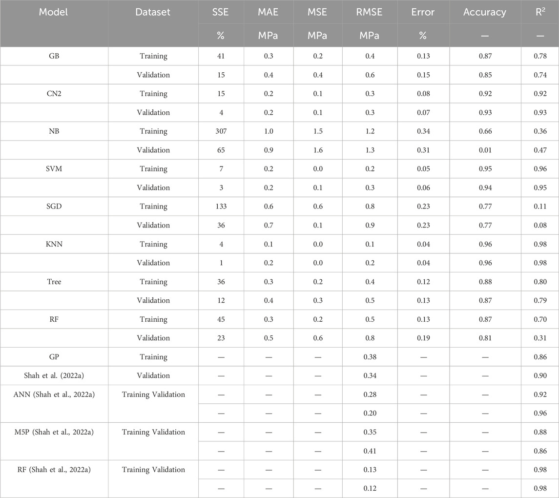
Table 2. Performance measurements of developed ensemble models for (Fsp).

4 Results presentation and discussion

4.1 GB model

The developed (GB) model was based on (Scikit-learn) method with learning rate of 0.1 and minimum splitting subset of 2. Nine trials were conducted for each model started with two trees and two tree levels and increased gradually to four trees and four tree levels. The reduction of the prediction error (%) for each trail is presented in Figure 4. Accordingly, the models with four trees and four tree levels are considered the optimum ones. This shows that the iterations based on the number of trees and levels below and above four did not produce desirable performance in terms errors and optimal concrete strength. Performance metrics of the developed model for both training and validation dataset are also presented. The average achieved accuracy was (86%). The relations between calculated and predicted values are shown in Figure 4.

Figure 4

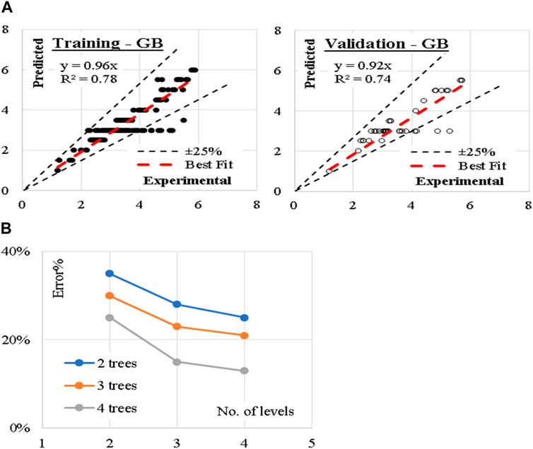
Figure 4. (A) Relation between predicted and calculated splitting tensile strength using (GB) and (B) Reduction in Error % with increasing the number of trees and levels.

4.2 CN2 model

Similarly, five (CN2) models were developed considering “Laplace accuracy” as evaluation measurement with beam width of 1.0 and minimum rule coverage of 1.0. The maximum rule length was started by 1.0 and increased up to 9.0. Figure 5 shows the reduction in Error % with increasing the rule length. Accordingly, rule length of 7.0 is considered. The developed models contain 115 “IF condition” rules, Figure 5 presents some of these rules. Performance metrics of the developed model for both training and validation dataset are also presented. The average achieved accuracy was (93%). The relations between calculated and predicted values are shown in Figure 5.

Figure 5

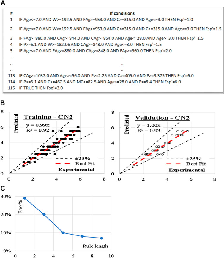
Figure 5. (A) Sample of the developed CN2 “If condition,” (B) Relation between predicted and calculated splitting tensile strength using (CN2) and (C) Reduction in Error % with increasing the rule length.

4.3 NB model

Traditional Naive Bayes classifier technique considering the concept of “Maximum likelihood” were used to develop the nine models. Although this type of classifier is highly scalable and are used in many applications, but it showed a very low performance as shown. The relations between calculated and predicted values are shown in Figure 6. The achieved average accuracies was33%.

Figure 6

Figure 6. Relation between predicted and calculated splitting tensile strength using (NB).

4.4 SVM model

The developed (SVM) model was based on “polynomial” kernel with cost value of 100, regression loss of 0.10 and numerical tolerance of 1.0. The kernel started with one-degree polynomial (linear) and increased up to three-degree polynomial (cubic). The reduction in the error % with increasing the polynomial degree is illustrated in Figure 7. Accordingly, (cubic) kernel is considered. Performance metrics of the three developed models for both training and validation dataset are also illustrated. The average achieved accuracy was (94%). The relations between calculated and predicted values are shown in Figure 7.

Figure 7

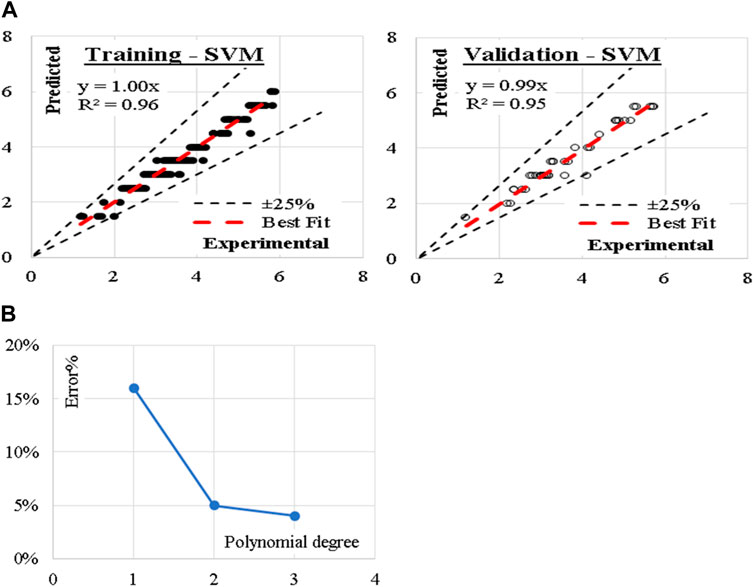
Figure 7. (A) Relation between predicted and calculated splitting tensile strength using (SVM) and (B) Reduction in Error % with increasing the polynomial degree.

4.5 SGD model

These three models were developed considering modified Huber classification function and “Elastic net” re-generalization technique with mixing factor of 0.01 and strength factor of 0.001. The learning rate, which is a crucial hyperparameter that controls the step size at each iteration of the optimization process starts with 0.01, then gradually decreased to 0.001. The reduction in error% with reducing the learning rate is presented in Figure 8. Performance metrics of the three developed models for both training and validation dataset are equally presented. The average achieved accuracy was (77%). The relations between calculated and predicted values are shown in Figure 8.

Figure 8

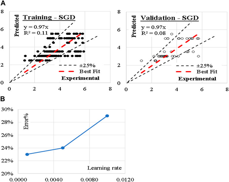
Figure 8. (A) Relation between predicted and calculated splitting tensile strength using (SGD) and (B) Reduction in Error % with reducing the learning rate.

4.6 KNN model

Considering number of neighbors of 1.0, Euclidian metric method and weights were evaluated by distances, the developed (KNN) models showed the best accuracy. (KNN) model showed the best performance where the average error (%) was (96%). The relations between calculated and predicted values are shown in Figure 9.

Figure 9

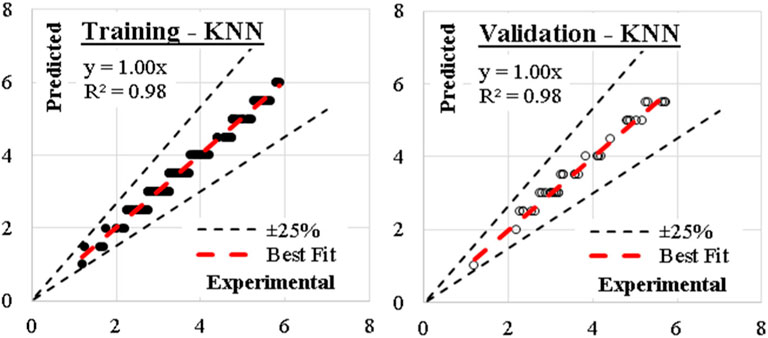
Figure 9. Relation between predicted and calculated splitting tensile strength using (KNN).

4.7 Tree model

These five models were developed considering minimum number of instants in leaves of 2.0 and minimum split subset of 5.0. The models began with only two tree levels and gradually increased to six levels. Figure 10 illustrates the reduction in Error % with increasing the number of layers. The layouts of the generated models are presented in Figure 10. Performance metrics of the last developed model for both training and validation dataset are also presented. The average achieved accuracy was (88%). The relations between calculated and predicted values are shown in Figure 10.

Figure 10

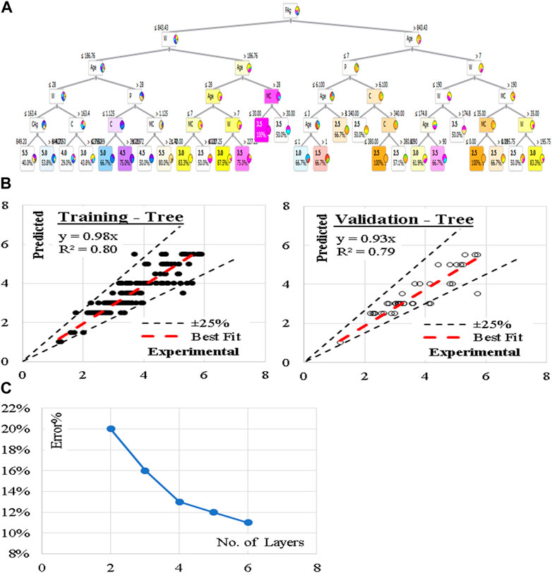
Figure 10. (A) The layout of the developed (Tree), (B) Relation between predicted and calculated splitting tensile strength using (Tree), and (C) Reduction in Error % with increasing the No. of layers.

4.8 RF model

Finally, nine (RF) models were generated. The models began with only two trees and two levels and increased up to four trees and four levels. Figure 11 shows the reduction in error (%) with increasing number of Tress and layers. Accordingly, the models with four trees and four layers are considered. The developed models are graphically presented using Pythagorean Forest in Figure 11. These arrangements leaded to a good average accuracy of (84%). The relations between calculated and predicted values are shown in Figure 11.

Figure 11

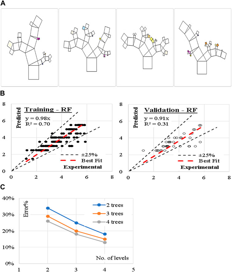
Figure 11. (A) Pythagorean Forest diagram for the developed (RF) models, (B) Relation between predicted and calculated splitting tensile strength using (RF) and (C) Reduction in Error % with increasing the No. of Tress and layers.

4.9 Ensemble models discussion

Overall, the performance measurements of developed ensemble models for the MK-mixed splitting tensile strength (Fsp) are presented in Table 2. It can be seen that the KNN outperformed the other techniques in the ensemble group with the following indices; SSE of 4% and 1%, MAE of 0.1 and 0.2 MPa, MSE of 0, RMSE of 0.1 and 0.2 MPa, Error of 0.04% and 0.04%, Accuracy of 0.96 and 0.96 and R2 of 0.98 and 0.98 for the training and validation models, respectively. This is followed closely by the SVM with the following indices; SSE of 7% and 3%, MAE of 0.2 and 0.2 MPa, MSE of 0.0 and 0.1 MPa, RMSE of 0.2 and 0.3 MPa, Error of 0.05% and 0.06%, Accuracy of 0.95 and 0.94, and R2 of 0.96 and 0.95, for the training and validation models, respectively. The third model in the superiority rank is the CN2 with the following performance indices; SSE of 15% and 4%, MAE of 0.2 and 0.2 MPa, MSE of 0.1 and 0.1 MPa, RMSE of 0.3 and 0.3 MPa, Error of 0.08% and 0.07%, Accuracy of 0.92 and 0.93 and R2 of 0.92 and 0.93, for the training and validation models, respectively. These models outperformed the GP, ANN, and M5P models utilized on the MK-mixed concrete found in the literature (Shah et al., 2022b), therefore are the better decisive modes for the prediction of the splitting strength (Fsp) of the studied MK-mixed concrete with 204 d mix data entries. However, the ANN used in the previous work performed with equal R2 of 0.98 of the present research work but the present work’s performance is better by comparing the RMSE values. Conversely, the NB and SGD produced unacceptable model performances, however, this is true for the modeled database collected for the MK-mixed Fsp. Figure 12 presents the comparison of the accuracies of the developed models for Fsp prediction using Taylor charts for the ensemble machine learning techniques. The performance of the models in this present research paper presents superior models compared to previous research papers, that presented model research results from genetic programming (GP), artificial neural networks (ANN), random forest (RF) and M5P tree models (Shah et al., 2022a; 2022b).

Figure 12

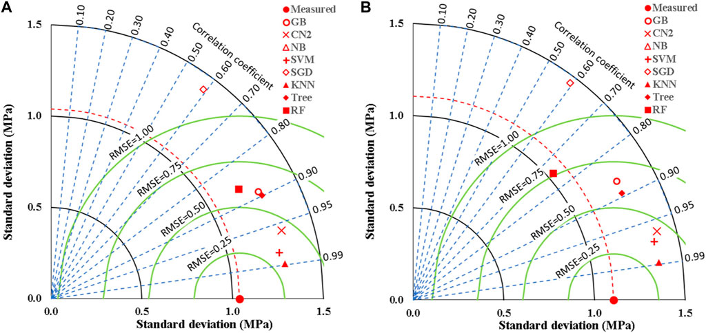
Figure 12. Comparing the accuracies of the developed models for (Fsp) using Taylor charts; (A) Training dataset, (B) Validation dataset.

4.10 RSM

The Model F-value of 41.67 implies the MK-mixed concrete Fsp model is significant. There is only a 0.01% chance that an F-value this large could occur due to noise. p-values less than 0.0500 indicate model terms are significant. In this case A, C, D, E, F, G, AC, AD, AE, AF, BC, BD, BE, BF, CD, CE, CG, DE, EF, FG, A², B², C², D², E², G² are significant model terms. Values greater than 0.1000 indicate the model terms are not significant. If there are many insignificant model terms (not counting those required to support hierarchy), model reduction may improve your model. The predicted R² of 0.9332 is in reasonable agreement with the Adjusted R² of 0.9752; i.e., the difference is less than 0.2. Adeq precision measures the signal to noise ratio. A ratio greater than four is desirable. Your ratio of 27.417 indicates an adequate signal. This performance corroborates with the results deposited in the literature (Ofuyatan et al., 2022). These presented results are summarized in the tables in the Supplementary Material. This model can be used to navigate the design space. Eq. 8 in terms of actual factors can be used to make predictions about the response for given levels of each factor. Here, the levels should be specified in the original units for each factor. This equation should not be used to determine the relative impact of each factor because the coefficients are scaled to accommodate the units of each factor and the intercept is not at the center of the design space. The RSM model simulation of the Fsp of the MK mixed concrete produced optimized scatter plots of residuals, runs, Cook’s distance, Box-Cox plots for power transforms, predicted and actual values of the Fsp, DFFITS and DFBETAS for the intercept to run configurations, and 3D surface configurations in Figures 13–18. In Figure 13, the RSM plot of the residuals, residuals versus predicted values, and residuals versus entry runs is illustrated. In Figure 14, the plot of the (a) Cook’s distance and (b) Box-Cox for power transforms is presented. In Figure 15, the plots of (a) predicted versus actual values, (b) residuals versus cement addition, (c) leverage versus run, (d) DFFITS versus run, and (e) DFBETAS for intercept versus run are presented. In Figure 16, the plots of the Fsp 3D surface for (a) MK-C combination, (b) W-C combination, (c) FAg-C combination, (d) CAg-C combination, (e) P-C combination, and (f) Age-C combination in the concrete mixes and presented. In Figure 17, the desirability of the optimized Fsp based on the best outcome from multiple iterations is illustrated. And finally, in Figure 18, the RSM Fsp behavioral scatter pattern with the single impacts of (a) C, (b) MK, (c) W, (d) FAg, (e) CAg, (f) P, and (g) Age. These plots represent the structural behavioral patter of the MK-mixed concrete splitting tensile strength (Fsp) with the introduction of the selected concrete components especially the supplementary cementitious activity of the MK.

$\begin{array}{l}\text{Fsp}=-228.37737+0.344850\mathrm{C}+0.356382\text{MK}+0.677729\mathrm{W}+0.171709\text{FAg}+0.072973\text{CAg\hspace{0.17em}}-0.385967\mathrm{P}\\ +0.036778\text{Age\hspace{0.17em}}-0.000059\mathrm{C}*\text{MK\hspace{0.17em}}-0.000764\mathrm{C}*\mathrm{W}-0.000068\mathrm{C}*\text{FAg\hspace{0.17em}}-0.000088\mathrm{C}*\text{CAg\hspace{0.17em}}-0.000973\mathrm{C}*\mathrm{P}\\ +0.000049\mathrm{C}*\text{Age\hspace{0.17em}}-0.000677\text{MK}*\mathrm{W}-0.000081\text{MK}*\text{FAg\hspace{0.17em}}-0.000146\text{MK}*\text{CAg\hspace{0.17em}}-0.001589\text{MK}*\mathrm{P}\\ +0.000098\text{MK}*\text{Age}-0.000211\mathrm{W}*\text{FAg\hspace{0.17em}}-0.000142\mathrm{W}*\text{CAg\hspace{0.17em}}-0.002061\mathrm{W}*\mathrm{P}-0.000105\mathrm{W}*\text{Age\hspace{0.17em}}-0.000034\text{FAg}*\text{CAg\hspace{0.17em}}\\ -0.000242\text{FAg}*\mathrm{P}+2.32722\mathrm{E}-06\text{FAg}*\text{Age}+0.001651\text{CAg}*\mathrm{P}-0.000011\text{CAg}*\text{Age\hspace{0.17em}}-0.001260\mathrm{P}*\text{Age\hspace{0.17em}}\\ -0.000088{\mathrm{C}}^2-0.000057{\text{MK}}^2-0.000163{\mathrm{W}}^2-0.000050{\text{FAg}}^2+6.93384\mathrm{E}-06{\text{CAg}}^2-0.001011{\mathrm{P}}^2-0.000121{\text{Age}}^2\end{array}(8)$

Figure 13

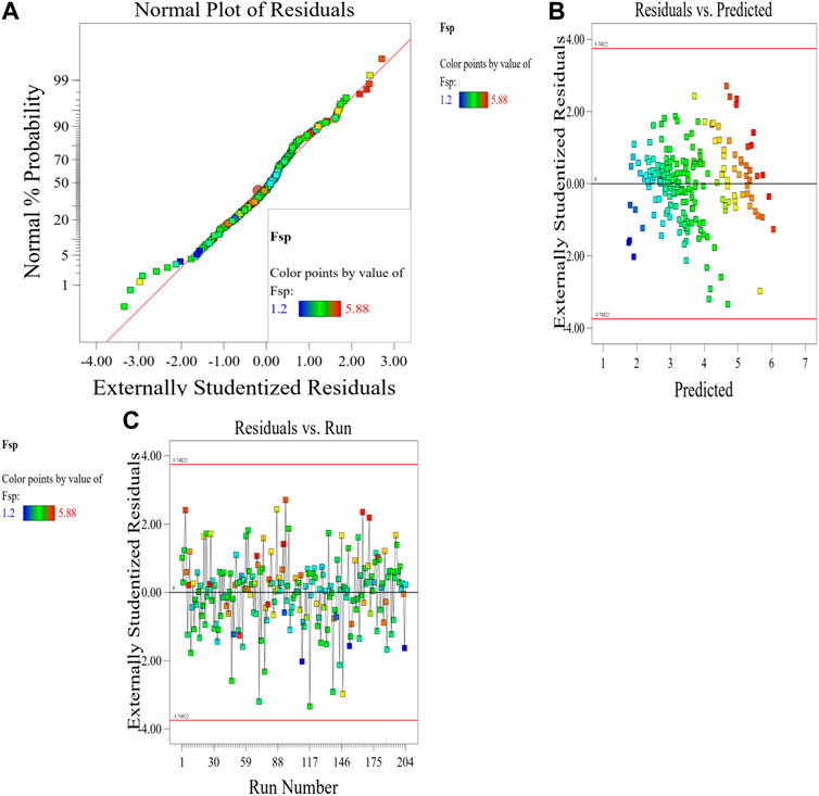
Figure 13. (A) RSM plot of the residuals, (B) residuals versus predicted values, and (C) residuals versus entry runs.

Figure 14

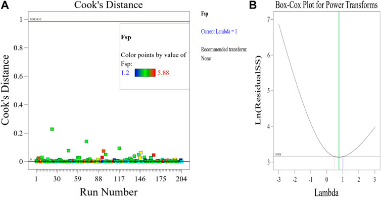
Figure 14. Plot of the (A) Cook’s distance and (B) Box-Cox for power transforms.

Figure 15

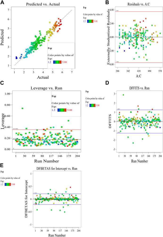
Figure 15. Plots of (A) predicted versus actual values, (B) residuals versus cement addition, (C) leverage versus run, (D) DFFITS versus run, and (E) DFBETAS for intercept versus run.

Figure 16

Figure 16. Plots of the Fsp 3D surface for (A) MK-C combination, (B) W-C combination, (C) FAg-C combination, (D) CAg-C combination, (E) P-C combination, and (F) Age-C combination in the concrete mixes.

Figure 17

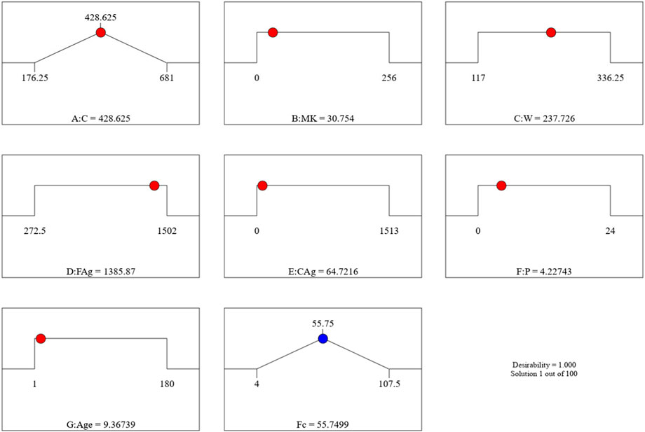
Figure 17. The desirability of the optimized Fsp based on the best outcome from multiple iterations.

Figure 18

Figure 18. RSM Fsp behavioral scatter pattern with the single impacts of (A) C, (B) MK, (C) W, (D) FAg, (E) CAg, (F) P, and (G) Age.

5 Conclusion

This research presents a comparative study between eight ML classification techniques, namely, GB, CN2, NB, SVM, SGD, KNN, Tree and RF to estimate the impact of adding meta-kaolin to concrete on its splitting strength considering mixture components contents and concrete age. The outcomes of this study could be concluded as follows:

- (CN2, SVM, KNN) models showed an excellent accuracy of about 93%–96%, while (GB, Tree, RF) models showed very good accuracies of about (84%–88%), (SGD) models showed fair accuracy level of about 77% and finally (NB) presented unacceptable accuracy (less than 50%).

- Both of correlation matrix and sensitivity analysis indicated that all considered inputs have almost the same level of impact on the splitting strength except the aggregate contents (CAg, FAg) which has almost neglected impact on the concrete splitting strength, this observation makes perfect sense since splitting strength is a kind of tensile strength which is mainly resisted by the binder and increased with time.

- The RSM model produced R2 of above 95% in addition to a closed-form equation, which allows the RSM model to be applied manually in addition. It also performed with an adequate precision of 27.4172, which outperforms the standard established for RSM models.

- All the developed models are too complicated to be used manually, which may be considered as the main disadvantage of the ML classification techniques compared with other symbolic regression ML techniques such as the RSM utilized in this work and GP and EPR presented in the literature.

- The developed models are valid within the considered range of parameter values, beyond this range; the prediction accuracy should be verified.

Data availability statement

The original contributions presented in the study are included in the article/Supplementary Material, further inquiries can be directed to the corresponding authors.

Author contributions

CG: Data curation, Project administration, Resources, Writing–original draft, Writing–review and editing. AA: Data curation, Investigation, Resources, Validation, Writing–review and editing. AS: Investigation, Methodology, Project administration, Resources, Visualization, Writing–original draft. NU: Investigation, Methodology, Project administration, Resources, Writing–original draft. AB: Formal Analysis, Investigation, Methodology, Resources, Supervision, Visualization, Writing–original draft. KO: Conceptualization, Data curation, Formal Analysis, Investigation, Methodology, Software, Supervision, Validation, Visualization, Writing–original draft, Writing–review and editing. AE: Investigation, Methodology, Project administration, Software, Visualization, Writing–original draft. SH: Data curation, Investigation, Project administration, Resources, Writing–original draft.

Funding

The authors declare that no financial support was received for the research, authorship, and/or publication of this article.

Conflict of interest

The authors declare that the research was conducted in the absence of any commercial or financial relationships that could be construed as a potential conflict of interest.

Publisher’s note

All claims expressed in this article are solely those of the authors and do not necessarily represent those of their affiliated organizations, or those of the publisher, the editors and the reviewers. Any product that may be evaluated in this article, or claim that may be made by its manufacturer, is not guaranteed or endorsed by the publisher.

Supplementary material

The Supplementary Material for this article can be found online at: https://www.frontiersin.org/articles/10.3389/fbuil.2024.1395448/full#supplementary-material

References

Al-alaily, H. S., and Hassan, A. A. A., Refined statistical modeling for chloride permeability and strength of concrete containing metakaolin, Constr. Build. Mater. 114 (2016) 564–579. doi:10.1016/j.conbuildmat.2016.03.187

CrossRef Full Text | Google Scholar

Barton, R. R. (2013). “Response surface methodology,” in Encyclopedia of operations research and management science. Editors S. I. Gass, and M. C. Fu (Boston, MA: Springer). doi:10.1007/978-1-4419-1153-7_1143

CrossRef Full Text | Google Scholar

de Oliveira, L. G., de Paiva, A. P., Balestrassi, P. P., Ferreira, J. R., da Costa, S. C., and da Silva Campos, P. H. (2019). Response surface methodology for advanced manufacturing technology optimization: theoretical fundamentals, practical guidelines, and survey literature review. Int. J. Adv. Manuf. Technol. 104, 1785–1837. doi:10.1007/s00170-019-03809-9

CrossRef Full Text | Google Scholar

Dinakar, P., Sahoo, P. K., and Sriram, G. (2013). Effect of metakaolin content on the properties of high strength concrete. Int. J. Concr. Struct. Mater. 7, 215–223. doi:10.1007/s40069-013-0045-0

CrossRef Full Text | Google Scholar

Ebid, A. (2020). 35 Years of (AI) in geotechnical engineering: state of the art. Geotech. GeolEng 39, 637–690. doi:10.1007/s10706-020-01536-7

CrossRef Full Text | Google Scholar

Güneyisi, E., Gesoğlu, M., and Mermerdaş, K. (2008). Improving strength, drying shrinkage, and pore structure of concrete using metakaolin. Mater. Struct. 41, 937–949. doi:10.1617/s11527-007-9296-z

CrossRef Full Text | Google Scholar

Hamby, D. M. (1994). A review of techniques for parameter sensitivity analysis of environmental models. Environ. Monit. Assess. 32, 135–154. doi:10.1007/BF00547132

PubMed Abstract | CrossRef Full Text | Google Scholar

Hoffman, F. O., and Gardner, R. H. (1983). “Evaluation of uncertainties in environmental radiological assessment models,” in Radiological assessments: a textbook on environmental dose assessment. Editors J. E. Till, and H. R. Meyer (Washington, DC: U.S. Nuclear Regulatory Commission). Report No. NUREG/CR-3332.

Google Scholar

Kannan, V., and Ganesan, K. (2014). Mechanical properties of self-compacting concrete with binary and ternary cementitious blends of metakaolin and fly ash. South Afr. Inst. Civ. Eng. Suid-Afrikaanse Inst. Siviele Ingenieurswese. 56, 97–105.

Google Scholar

Khan, R. A., and Haq, M. (2020). Long-term mechanical and statistical characteristics of binary-and ternary-blended concrete containing rice husk ash, metakaolin and silica fume. Innov. Infrastruct. Solut. 5, 53–14. doi:10.1007/s41062-020-00303-0

CrossRef Full Text | Google Scholar

Ofuyatan, O. M., Agbawhe, O. B., Omole, D. O., Igwegbe, C. A., and Ighalo, J. O. (2022). RSM and ANN modelling of the mechanical properties of self-compacting concrete with silica fume and plastic waste as partial constituent replacement. Clean. Mater. 4, 100065. doi:10.1016/j.clema.2022.100065

CrossRef Full Text | Google Scholar

Onyelowe, K. C., and &Ebid, A. M. (2023). The influence of fly ash and blast furnace slag on the compressive strength of high-performance concrete (HPC) for sustainable structures. Asian J. Civ. Eng. 25, 861–882. doi:10.1007/s42107-023-00817-9

CrossRef Full Text | Google Scholar

Onyelowe, K. C., Ebid, A. M., and &Ghadikolaee, M. R. (2023c). GRG-optimized response surface powered prediction of concrete mix design chart for the optimization of concrete compressive strength based on industrial waste precursor effect. Asian J. Civ. Eng. 25, 997–1006. doi:10.1007/s42107-023-00827-7

CrossRef Full Text | Google Scholar

Onyelowe, K. C., Ebid, A. M., Mahdi, H. A., Onyelowe, F. K. C., Shafieyoon, Y., Onyia, M. E., et al. 2023a, “AI mix design of fly ash admixed concrete based on mechanical and environmental impact considerations”, Civ. Eng. J., Vol. 9, Special Issue, 2023, 27, 45. doi:10.28991/CEJ-SP2023-09-03

CrossRef Full Text | Google Scholar

Onyelowe, K. C., Ebid, A. M., Mahdi, H. A., Soleymani, A., Jahangir, H., and Dabbaghi, F. (2022d). Optimization of green concrete containing fly ash and rice husk ash based on hydro-mechanical properties and life cycle assessment considerations. Civ. Eng. J. 8 (12), 3912–3938. doi:10.28991/CEJ-2022-08-12-018

CrossRef Full Text | Google Scholar

Onyelowe, K. C., Ebid, A. M., Riofrio, A., Soleymani, A., Baykara, H., Kontoni, D.-P. N., et al. (2022c). Global warming potential-based life cycle assessment and optimization of the compressive strength of fly ash-silica fume concrete; environmental impact consideration. Front. Built Environ. 8, 992552. doi:10.3389/fbuil.2022.992552

CrossRef Full Text | Google Scholar

Onyelowe, K. C., Gnananandarao, T., Ebid, A. M., Mahdi, H. A., Razzaghian-Ghadikolaee, M., and Al-Ajamee, M. (2022b). Evaluating the compressive strength of recycled aggregate concrete using novel artificial neural network. Civ. Eng. J. 8 (8), 1679–1693. doi:10.28991/CEJ-2022-08-08-011

CrossRef Full Text | Google Scholar

Onyelowe, K. C., Gnananandarao, T., Jagan, J., Ahmad, J., and &Ebid, A. M. (2022e). Innovative predictive model for flexural strength of recycled aggregate concrete from multiple datasets. Asian J. Civ. Eng. 24, 1143–1152. doi:10.1007/s42107-022-00558-1

CrossRef Full Text | Google Scholar

Onyelowe, K. C., Kontoni, D.-P. N., Ebid, A. M., Dabbaghi, F., Soleymani, A., Jahangir, H., et al. (2022a). Multi-objective optimization of sustainable concrete containing fly ash based on environmental and mechanical considerations. Buildings 2022, 948. doi:10.3390/buildings12070948

CrossRef Full Text | Google Scholar

Onyelowe, K. C., Mojtahedi, F. F., Ebid, A. M., Rezaei, A., Osinubi, K. J., Eberemu, A. O., et al. (2023b). Selected AI optimization techniques and applications in geotechnical engineering. Cogent Eng. 10 (1)–2153419. doi:10.1080/23311916.2022.2153419

CrossRef Full Text | Google Scholar

Ray, S., Haque, M., Rahman, M. M., Sakib, M. N., and Al Rakib, K., Experimental investigation and SVM-based prediction of compressive and splitting tensile strength of ceramic waste aggregate concrete, J. King Saud. Univ.- Eng. Sci. 36, 112, 121. (2021). doi:10.1016/j.jksues.2021.08.010

CrossRef Full Text | Google Scholar

Ray, S., Rahman, M. M., Haque, M., Hasan, M. W., and Alam, M. M., Performance evaluation of SVM and GBM in predicting compressive and splitting tensile strength of concrete prepared with ceramic waste and nylon fiber, J. King Saud. Univ. - Eng. Sci. 35 (2023) 92–100. doi:10.1016/j.jksues.2021.02.009

CrossRef Full Text | Google Scholar

Shah, H. A., Nehdi, M. L., Khan, M. I., Akmal, U., Alabduljabbar, H., Mohamed, A., et al. (2022a). Predicting compressive and splitting tensile strengths of silica fume concrete using M5P model tree algorithm. Mater. (Basel) 15, 5436. doi:10.3390/ma15155436

CrossRef Full Text | Google Scholar

Shah, H. A., Yuan, Q., Akmal, U., Shah, S. A., Salmi, A., Awad, Y. A., et al. (2022b). Application of machine learning techniques for predicting compressive, splitting tensile, and flexural strengths of concrete with metakaolin. Mater. (Basel) 15, 5435. doi:10.3390/ma15155435

CrossRef Full Text | Google Scholar