Enhanced seagull optimization for enhanced accuracy in CUDA-accelerated Levenberg–Marquardt backpropagation neural networks for earthquake forecasting

Hyperparameter tuning is crucial for enhancing the accuracy and reliability of artificial neural networks (ANNs). This study presents an optimization of the Levenberg–Marquardt backpropagation neural network (LM-BPNN) by integrating an improved seagull optimization algorithm (ISOA). The proposed ISOA-LM-BPNN model is designed to forecast earthquakes in the Caribbean region. The study further explores the impact of data and model parallelism, revealing that hybrid parallelism effectively mitigates the limitations of both. This leads to substantial gains in throughput and overall performance. To address computational demands, this model leverages the compute unified device architecture (CUDA) framework, enabling hybrid parallelism on graphics processing units (GPUs). This approach significantly enhances the model’s computational speed. The experimental results demonstrate that the ISOA-LM-BPNN model achieves a 20% improvement in accuracy compared to four baseline algorithms across three diverse datasets. The integration of ISOA with LM-BPNN refines the neural network’s hyperparameters, leading to more precise earthquake predictions. Additionally, the model’s computational efficiency is evidenced by a 56% speed increase when utilizing a single GPU, and an even greater acceleration with dual GPUs connected via NVLink compared to traditional CPU-based computations. The findings underscore the potential of ISOA-LM-BPNN as a robust tool for earthquake forecasting, combining high accuracy with enhanced computational speed, making it suitable for real-time applications in seismic monitoring and early warning systems.

1 Introduction

The unpredictable, sporadic, and erratic nature of seismic activity presents significant difficulties for earthquake preparedness. The abrupt shifts in tectonic behavior within brief intervals can lead to catastrophic seismic events. Hence, precisely forecasting seismic movements is essential for anticipating earthquake magnitudes and ensuring the stability and safety of affected regions. Artificial neural networks (ANNs) are a class of machine learning models inspired by the structure and function of the human brain. ANNs consist of interconnected layers of nodes, or “neurons,” which work together to process input data, learn patterns, and make predictions. These networks are particularly effective in handling complex, non-linear relationships within data, making them suitable for a wide range of applications, including image recognition, natural language processing, and, notably, earthquake forecasting. The architecture of an ANN typically includes an input layer, one or more hidden layers, and an output layer. Each neuron in a layer is connected to neurons in the subsequent layer through weighted connections. During the training process, the network adjusts these weights based on the error of its predictions—a process known as “backpropagation”. This iterative adjustment allows the network to learn from the data and improve its accuracy over time. To forecast an earthquake using an ANN requires efficient precursors and fine tuning the hyper-parameters of an algorithm.

The process of selecting the right hyperparameters is crucial for the performance of machine learning (ML) models. A suboptimal choice can diminish the accuracy of the model (Bergstra and Bengio, 2012). Moreover, the tuning of hyperparameters, involving the exploration of a wide parameter space, is often computationally intensive and time-consuming (Jasper et al., 2012). Properly navigating this trade-off is essential for efficient model development and deployment.

Furthermore, as artificial intelligence advances, its techniques demonstrate significant potential in discerning the nonlinear patterns of seismic activity. Such methods are increasingly pivotal in earthquake forecasting research. Approaches like ML, ANNs, support vector machines (SVMs) (Kollam and Joshi, 2020), and fuzzy logic (FL) methods have been explored for predicting seismic events.

Xiong et al. (2021) used satellite data for ML in earthquake forecasting. This suggested approach for earthquake forecasting employs cross-validation and hyperparametric optimization to identify the optimal model parameters. Xiong et al. (2021) used an inverse boosting pruning trees (IBPT) ML approach to study the physical and dynamic changes in environmental effects occurring in the short-term using satellite data to anticipate earthquakes of magnitude 6 or higher.

Gitis and Derendyaev (2019) introduced a ML technique for forecasting seismic hazards. This considers two kinds of approaches: spatial forecasting to find the maximum seismic event, and considering spatio-temporal forecasting for a web-based earthquake forecasting system to find the location of an earthquake.

Jena et al. (2020) assessed earthquake risk and hazard at Palu, Indonesia, using ML techniques. They used AHP and weighted overlay methods to measure vulnerability, and CNN was used to estimate likelihood. Despite the limitations of that study, the strategy was valuable for ERA and successful for catastrophe risk reduction.

Mousavi and Beroza (2020) suggested an ML method for calculating earthquake magnitude. In that study, a rapid and precise method for estimating earthquake magnitude from beginning to end utilizing unprocessed waveforms gathered at single stations was described. They detailed a rapid and precise method for estimating earthquake magnitude from beginning to end utilizing unprocessed waveforms gathered at single stations. This method has several potential uses, including routine seismic monitoring and early warning systems.

Rundle et al. (2021) recommend a novel earthquake nowcasting using ML on the California earthquake cycle to visualize the temporally dependent earthquake cycle. The method involves imaging the earthquake cycle time-dependently to correspond with stress accumulation and release. This can help identify periods of increased seismic activity and potential earthquake clusters. Principal component analysis (PCA) seismic activity of area is considered to construct time-series. The patterns were identified as eigenvectors of the cross-correlation matrix of a collection of seismicity time series utilizing a geographical grid.

Aslam et al. (2021) used a cutting-edge ML approach to predict earthquake activity in northern Pakistan. They employs seismological concepts, including seismic quiescence, the inverse law of Gutenberg–Richter, and the extent of earthquakes to analyze eight seismic characteristics for the purpose of earthquake prediction in the Hindu Kush. A classification framework is proposed that utilizes a support vector regressor (SVR) and a hybrid neural network (HNN) to predict earthquakes.

Asim et al. (2020) examined the prediction of seismic activity in Cyprus using short-term forecasting, seismicity analysis, and ML algorithms. They used the temporal analysis of the earthquake catalogue and eliminated noisy data. The internal seismic status of the area was then expressed using 60 seismic characteristics based on a cleaned earthquake dataset. The related seismic activity was then modeled alongside these seismic properties using ML techniques.

Xiong et al. (2020) conducted an analysis of ionospheric disturbances detected before significant seismic occurrences using data obtained from the DEMETER satellite. They examined 16 classification methods for this purpose. The LightGBM technique, which is based on gradient boosting, demonstrated superior performance over other algorithms in identifying electromagnetic pre-earthquake disturbances (Xiong et al., 2020). The strength of its performance was underscored via a thorough five-fold cross-validation examination using standard datasets. The choice of geographic area utilized in crafting the training set for non-seismic data noticeably influences the efficacy of the LightGBM model, albeit within certain limits.

Cui et al. (2021) introduced a strategy for predicting earthquake casualties based on stacking. Numerous factors affect the number of fatalities, making a thorough technique for predicting earthquake casualties necessary. In this study, an efficient prediction approach based on an upgraded swarm intelligence algorithm using stacking ensemble learning was suggested to produce reliable prediction results.

Deep learning (DL) involves employing artificial neural networks with several hidden layers to discern patterns in expansive and often high-dimensional data sets (Khan et al., 2019). These intricate networks are honed for a diversity of applications, such as categorizing images (Nibha and Burris, 2019), analyzing text (Chatterjee et al., 2019), and interpreting speech (Ravanelli et al., 2020). The depth and complexity of these networks permit a nuanced understanding and representation of data, making them an essential tool in various research domains. Deep neural networks (DNNs), when trained on expansive datasets, necessitate substantial computational resources to execute gradient descent and adjust weights effectively. Multiple efforts have been directed at minimizing their computational burden and refining their processing efficiency (Singh et al., 2017). The challenge lies not just in data handling but also in optimizing the learning process without compromising the integrity of the model’s performance.

In training ANNs, the use of GPUs has increased tremendously (Zhang et al., 2018; Nibha and Burris, 2019). To reduce computing time in training data, the NVIDIA has introduced a framework called CUDA to execute programs in parallel using GPU cores (Zukovic et al., 2020; Sanders and Kandrot, 2010). There are two types of parallelization possible. The first is data parallelization, where the data is divided into multiple subsets and given to the different cores in the GPU to execute the same model (Danielsson et al., 2018). The second is model parallelization, where the model/algorithm is divided and given to the different nodes, but the data is not divided (Venkata Divya and Sai Prasad, 2018).

The DNN training parameter’s mini-batch size is affected by the data partition size for data parallelism (Florido et al., 2018). If too big, a mini batch size can boost GPU utilization but decrease model accuracy. On the other hand, the GPU’s resources are underutilized when batches are small. When data parallelism is used, the effective mini batch size equals the number of GPUs times the mini batch size. To overcome the drawbacks of a high mini batch size, we might divide it among GPUs (López-Martínez et al., 2023), but this may underutilize GPU resources. Efficient DNN training using GPUs becomes harder on a selected data size as GPUs increase.

Pipelined training causes staleness in model parallelism. Since numerous mini batches are in progress, later ones use stale weights to generate gradients before updating weights. The staleness issue causes inconsistent learning and poor model accuracy. Model accuracy (correct classifications) comparisons between models and data parallelism shows that the accuracy of the latter rises with training, whereas model parallelism accuracy varies (Chen et al., 2019).

Previous studies that have focused on different ML approaches (e.g., SVMs, CNNs, LSTMs, LightGBM) have often overlooked the computational efficiency and accuracy of the model; this research highlights both improvements in accuracy and enhancements in computational speed.

In this study, we propose an improved seagull optimization algorithm (ISOA) integrated with LM-BPNN to develop a highly accurate and computationally efficient model for earthquake forecasting. By leveraging the compute unified device architecture (CUDA) framework for parallel processing on graphics processing units (GPUs), we can further accelerate the training process by enabling real-time applications in seismic monitoring.

2 Materials and methods

We focused on the ISO-LM-BPNN using CUDA framework. The Figure 1 block diagram gives an overview of the proposed methodology.

Figure 1

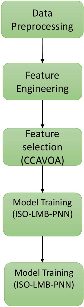
Figure 1. Block diagram of proposed methodology.

2.1 Seagull optimization algorithm

In the diverse and evolving landscape of optimization algorithms, nature-inspired metaheuristics have emerged as potent tools to tackle complex optimization problems. These algorithms often draw inspiration from the intricate and adaptive behaviors exhibited by various organisms, ranging from the choreographed dances of bees to the synchronized schooling of fish. Amidst this array of bio-inspired algorithms, the seagull optimization algorithm (SOA) was modeled after the foraging behaviors of seagulls (Dhiman and Kumar 2019). Seagulls, renowned for their extensive foraging range, exhibit a dualistic search mechanism. They can scour for food on the sea’s surface or dive beneath to catch prey. This dual strategy, encompassing both exploration and exploitation, is what the SOA aims to capture and mathematically model for optimization tasks.

When using SOA, “pop” is the population number of the seagulls, $D^{,}$ is the dimension of the issue space, and “$a_i$ = ($a_i^1$, $a_i^2$,.., $a_i^{D^{,}}$), i = 1, 2, pop” is the location of the seagull. The act of updating each individual’s position is what drives the seagull movement and attack behavior.

2.1.1 Migration behavior

The global search encompasses migratory behavior. Seagulls migrate when they travel from one location to another, but there are three requirements they must meet: avoid collisions, fly in the direction of the best position, and approach the ideal location.

2.1.1.1 Avoiding collisions

An extra variable $Q$ is added to prevent collisions between neighboring seagulls. The program updates the seagull’s location in the iterative process concurrently using this variable.

${ct}_{iter}=Q\times {IP}_{iter}(1)$

where ${IP}_{iter}$ is the seagull’s initial position, iter is the current iteration number, ${ct}_{iter}$ is the seagull’s new position after avoiding collisions, and Q is the seagull’s motion pattern inside a certain search area. Q’s equation is:

$Q=f_g^{\prime }-(iter\times \left(\frac{f_g^{\prime }}{{\mathit{max}}_{iter}}\right)(2)$

where ${\mathit{max}}_{iter}$ is the maximum number of iterations, $f_g^{\prime }$ is reduced linearly to zero, and the value of Q is modified linearly.

2.1.1.2 Direction of the best position

The seagull will fly in the direction of the best position once it is confident it will not crash with any other birds. The formula reads as follows:

$m_{iter}=R\times \left({C\left(best\right)}_{iter}-{IP}_{iter}\right)(3)$

$R=2\times Q\times Q\times r_n(4)$

where ${C\left(best\right)}_{iter}$ denotes the best location in the population, $R$ is a random integer that balances local and global search, and the value of $r_n$ is a random number of (0,1).

2.1.1.3 Approaching the best position

The seagull flies in the direction of the best position to reach a new location after moving to a place where it avoids colliding with other seagulls.

${f\left(best\right)}_{iter}=\left|{C\left(best\right)}_{iter}+m_{iter}\right|(5)$

where ${f\left(best\right)}_{iter}$ represents the best fit search seagull.

2.2.1 Attack behavior

The attack behavior is local search-related. Using a, b, and c to describe their movements, seagulls attack their prey by spiraling in the air. The exercise behavior equation is as per Equations 6–9,

$a=s_r\times \mathit{cos}\theta (6)$

$b=s_r\times \mathit{sin}\theta (7)$

$c=s_r\times \theta (8)$

$s_r=\phi \times e^{\theta s_c}(9)$

where $s_r$ is the spiral’s radius when the seagull is flying, and $s_c$ are the spiral’s correlation constants. The angle is represented as a random integer between [0, 2]. Equation 10 describes how seagulls attack:

${IP}_{iter}={f\left(best\right)}_{iter}\times a\times b\times c+{C\left(best\right)}_{iter}(10)$

where ${IP}_{iter}$ updates the position of other search seagulls and stores the best answer.

2.1.3 The Steps of the SOA

Refer to the steps of SOA in Figure 2.

Figure 2

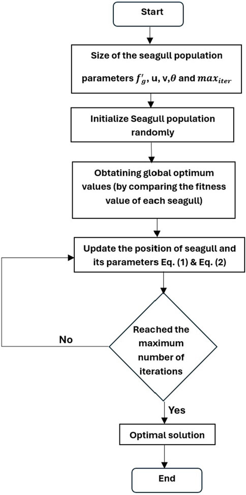
Figure 2. Flow chart of SOA.

2.2 Improved seagull optimization algorithm

The ISOA benefits from a strong optimization impact, ease of use, and minimal parameter settings. SOA exhibits an early trend and is prone to local optimal behavior. It falls within the local search stage for Equation 8, which is prone to local extremes and may not provide the global optimum value (Ragab et al., 2022). To overcome local extremes, Equation 10 includes a cognitive component. Equation 10 has been improvised as:

${IP}_{iter}={f\left(best\right)}_{iter}\times a\times b\times c+{C\left(best\right)}_{iter}+{C\left(best\right)}_{iter}-{IP}_{iter}\times I_f(11)$

where $I_f$ stands for the inertia factor; in this study, its value is 0.95. $I_f$'s function is to increase each seagull’s capacity to find the global optimization instead of local minima.

We retain the best seagulls and reject the worst to get the best value. The seagull population is sorted from best to worst as per fitness values computed for each iteration; the best half of the seagull population is considered while the second half is discarded, helping to retain the best fitness value for the seagulls. The solution accuracy of the seagull optimization technique is not very great, and it is simple to fall into local extremes. The enhanced seagull optimization method, however, incorporates a cognitive component and a natural selection process to increase the system’s capacity to solve problems and prevent it from tumbling into local extremes.

Changing parameter R from Equation 4 from a linear to an exponential function controls the optimal position.

$R=e^Q{r}_n(12)$

Introduce ω, a weight parameter.

$\mathrm{\omega }=\left\{\begin{array}{l}\omega \mathit{max}-\left(\omega \mathit{max}\right){\left(\frac{{IP}_{iter\left(best\right)}-{IP}_{iter\left(avg\right)}}{{IP}_{iter\left(best\right)}}\right)}^{\frac{t}{T}},iter<D^{,}\ast 0.8\\ \omega \mathit{max},other\end{array}\right.,(13)$

${IP}_{iter}={\left(1-\omega \right)f\left(best\right)}_{iter}\times a\times b\times c+{C\left(best\right)}_{iter}+{C\left(best\right)}_{iter}-{IP}_{iter}\times I_f(14)$

Parameter:

Population number of the seagulls, D′

$a_i=\left(a_i^1,a_i^2,..,a_i^{D^{,}}\right),\mathrm{i}=1,2$, pop is the location of the seagull.

Extra variable Q is added to prevent collisions between neighboring seagulls.

Where ${IP}_{iter}$ is the seagull’s initial position,

$iter$ is the current iteration number, and

${ct}_{iter}$ is the seagull’s new position.

2.3 CUDA-accelerated LM-BPNN

A neural network consists of an input layer, an output layer, and a number of hidden layers based on the problem. A layer is comprised of a collection of neurons and associated weights, together with an activation function. The layers seen in Figure 3 are interconnected with subsequent levels. Each of these layers comprises several neurons. A problem’s complexity is determined as the number of hidden layers used in neural network (Ghorpade-Aher et al., 2012). Matrix multiplication plays a crucial role in contemporary deep neural network (DNN) methods, accounting for around 70%–80% of the computational burden throughout the DNN training process (Rao and Ramana, 2019). This is mostly due to the frequent repetition of matrix multiplication operations during DNN training. The effective implementation of matrix multiplication may be achieved through data parallelism, particularly by employing CUDA for parallel execution on a GPU. In our prior research, we employed the expedited Winograd’s matrix multiplication technique, the accelerated parallel Winograd’s matrix multiplication method, and the parallel blocked matrix multiplication approach with a collapse clause to enhance the efficiency of training DNN algorithms (Rao and Ramana, 2019). The objective of this study is to empirically demonstrate that matrix multiplication on a GPU using the CUDA framework represents a significant advancement in computing compared to other methods such as the standard (sequential) approach, the CBLAS library subroutine on a central processing unit (CPU), and the CUBLAS library.

Figure 3

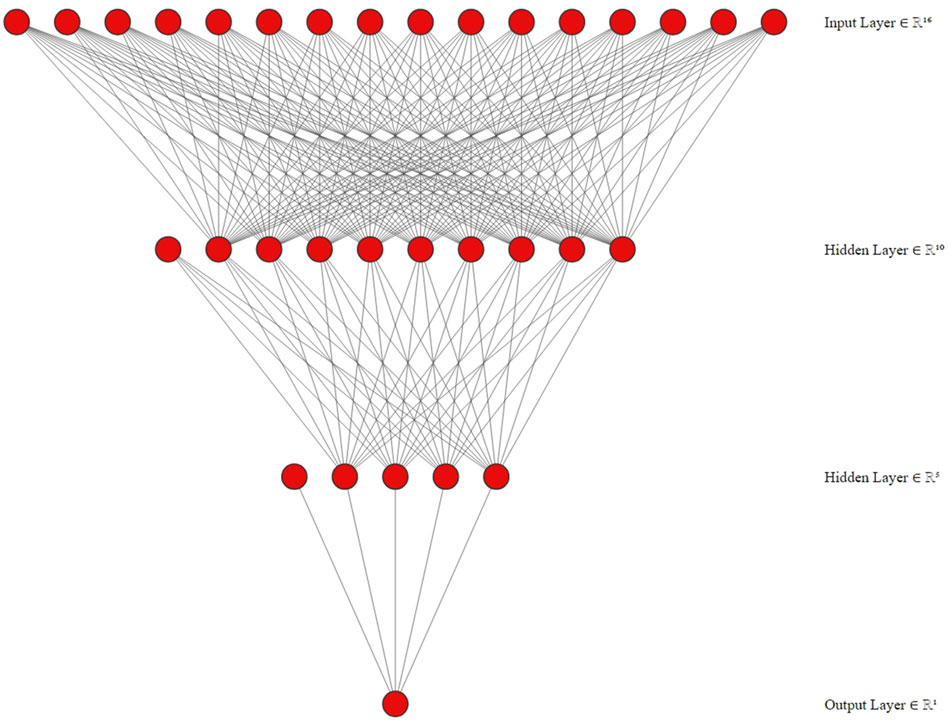
Figure 3. Structure of neural network with two hidden layers.

The primary mechanism for refining the weights and biases within the neurons of BPNN is the error backpropagation process.

The back-propagation algorithm operates in two distinct phases: training and testing (Lin et al., 2018). During the training phase, the algorithm employs a feed-forward pass wherein an input vector is introduced into the network and is sequentially processed through the layers to produce an output (Murata et al., 1994). Following this, in the back-propagation phase, the resultant output of the network is juxtaposed with the expected output. Discrepancies between the two leads to the computation of an error. Subsequently, this error information is used to adjust the network’s weights, ensuring that the model refines its predictions in future iterations, as delineated by the error correction rule (Bandala et al., 2015).

The Levenberg–Marquardt (LM) algorithm, traditionally utilized in nonlinear least squares problems, has been well adapted to train feed-forward neural networks. The amalgamation of the LM method with traditional backpropagation offers a potent mechanism for neural network training, providing faster convergence than conventional gradient descent-based approaches (Zhou et al., 2018; Amin et al., 2019). The gradient descent method and its variants have been the cornerstone of these training processes, guiding the weight adjustments based on the error gradient. However, gradient descent, although straightforward, often suffers from slow convergence, especially in regions of the error surface where the gradient is small. This limitation led to the exploration of second-order methods, and the LM algorithm emerged as a leader in this domain.

Gauss–Newton is used to obtain the second derivative (Hessian matrix), and the gradient descent method is used to adjust the weights by the first derivative error. Both methods are combined to create to develop the LM algorithm (M, Sarepaka, and P 2013).

The principal drawback of using LM-BPNN is memory-intensive and computational complexity. The LM algorithm requires the computation and storage of the Jacobian matrix, which can be memory-intensive for large networks, and inverting the matrix in the weight update equation can also be computationally expensive. Combining the seagull optimization algorithm (SGO) with the CUDA-accelerated LM backpropagation neural network (LM-BPNN) and hybrid-parallelization approach helps address this drawback.

Hybrid parallelism was implemented to achieve significant computational enhancement for the improved seagull optimization algorithm (ISOA) integrated with LM-BPNN. Hybrid parallelism combines data parallelism and model parallelism, effectively utilizing the computational power of GPUs to improve both speed and efficiency.

Data parallelism involves splitting the dataset into smaller chunks and distributing these across multiple GPU cores. Each core processes its assigned data chunk simultaneously using the same model, thereby significantly speeding up the data processing phase. Model parallelism, on the other hand, divides the neural network model into smaller sub-networks (SNNs). Each sub-network is processed independently on different GPU cores, allowing different parts of the model to be trained concurrently.

For instance, the neural network in our study was divided into two sub-networks. Sub-network 1 included the input layer and the first two hidden layers, while sub-network 2 comprised the third hidden layer and output layer. During the forward pass, each sub-network processed its respective part of the data in parallel. The outputs from sub-network 1 were passed to sub-network 2, maintaining the data flow required for sequential layers. In the backward pass, gradients were calculated independently within each sub-network and synchronized before updating the weights. This approach minimized computational bottlenecks associated with sequential processing and maximized GPU utilization.

The CUDA framework was employed to set up the GPU environment, specifying the number of threads and blocks for parallel execution. By leveraging CUDA for both data and model parallelism, the hybrid parallelism approach significantly reduced computational time. This method allowed for faster convergence of the neural network training process, as evidenced by a 56% speed increase when utilizing a single GPU and even greater improvements with dual GPUs connected via NVLink. The reduction in training time and the efficient utilization of GPU resources led to an overall 33% improvement in throughput compared to traditional CPU-based computations.

The integration of hybrid parallelism into the ISOA-LM-BPNN model thus provided substantial computational enhancements. It not only improved the speed of training but also ensured that the model maintained high accuracy levels, making it suitable for real-time applications in seismic monitoring and other domains requiring rapid and reliable computation.

For the calculation of grid blocks size,

$blocks=\lceil \frac{M}{t}\rceil (15)$

where M is size of the matrix, t is the maximum number of threads considered for use in the GPU.

$threads=\lfloor \frac{M}{blocks}\rfloor (16)$

thread block is calculated from Equation 16. The weight update for NN is

$W_{ij}=\gamma \frac{W_{ij}}{\sqrt{{\sum }_{i=1}^{n1}{W_{ij}}^2}}(17)$

2.4 Proposed ISO-LMT-BPNN prediction model

 Step 1: Input data.

 Step 2: Split data into data chunks (Di) (i=1,2,3,…..,n).

 Step 3: Calculate threads and grids (Equations 15, 16).

 Step 4: Parameters initialized for algorithm (ISOA).

 Step 5: Copy data to the GPU.

 Step 6: Map parameters to LM-BPNN and calculate its fitness evaluation for each SNN_i, $f\left(best\right)$.

 Step 7: For each SNN_i, update weight parameters by Equation 17,  update ${ct}_{iter}$ by Equation 1,  update $m_{iter}$ by Equation 3,  update ${IP}_{iter}$ by Equation 14.

 Step 8: Select best ${IP}_{iter}$ using LM optimization to refine weights and biases of each SNN_i.

 Step 9: Replace the best ${IP}_{iter}$ with optimized values by LM optimization in each SNN_i.

 Step 10: Take average of all c from each SNN_i.

 Step 11: If stopping criterion is met, go to Step 10; otherwise, go to Step 6.

 Step 12: The best ${IP}_{iter}$ with fitness values will have the best set of weights and biases for LM-BPNN.

2.5 Performance metrics

Utilizing performance metrics including accuracy, precision, recall, F-measure, RMSE, MAE, and MAPE, the suggested model’s performance is assessed (Kollam and Joshi, 2020).

a) Accuracy

The accuracy rate is calculated by the proportion of properly predicted instances to all examples. The accuracy is defined as,

$Accuracy=\frac{TP+TN}{TP+FP+FN+TN}(18)$

b) Precision

“Precision” refers to the accurate representation of the total number of genuine samples that are appropriately considered throughout the classification process relative to the total number of samples involved in the classification process.

$Precision=\frac{TP}{TP+FP}(19)$

c) Recall

The recall rate is a metric that quantifies the proportion of actual samples that are correctly identified while categorizing data using all samples from the training data within the same categories.

$Recall=\frac{TP}{TP+FN}(20)$

d) F- score

A single type of data item must be present in each class, and all data bits must be completely identified. The F-score number achieves this balance. It is defined as the harmonic mean of precision and recall rate.

$F_{Score}=\frac{2Precision\times Recall}{Precision+Recall}(21)$

e) RMSE

For each data point, obtain the residual (difference between forecast and reality), the norm of residual, the mean of residuals, and then take the square root of that mean to determine the root mean standard error (RMSE).

$RMSE=\sqrt{\frac{1}{N}{\left(p_i-q_i\right)}^2}(22)$

Here $p_i,q_i$ are the predicted and observed samples, respectively.

f) MAE

The mean absolute error (MAE) is a performance metric used in regression analysis to quantify difference between the absolute and predicted value.

$MAE=\frac{{\sum }_{j=1}^N\left|A_i-F_i\right|}{N}(23)$

g) MAPE

Utilizing the MAPE formula, demand is divided by the total number of distinct absolute errors (each period separately). It reflects an average of percentage errors.

$MAPE=\frac{1}{N_i}{\sum }_{i=1}^{N_i}\left|\frac{{Av}_i-{Fv}_i}{{Av}_i}\right|(24)$

Where, $N_i$ is the number of times the summation iteration occurs, ${Av}_i$ is the actual value, and ${Fv}_i$ is the forecast value.

h) Computation time (CT)

The time it takes to anticipate an earthquake’s magnitude is known as the CT. where TE is the end time of the algorithm and TS its start time on CPU and GPU.

$\text{CT}=\text{TE}-\text{TS}(25)$

2.6 Experiment setup

In this section, we used three different datasets to conduct the experiment. Datasets are the earthquake database from USGS (Survey, 2020), IRIS database (150 × 4) (Fisher, 1988), and traffic-flow prediction (2101 × 47) (Zhao, 2021); they can be found in the UCI ML repository. The hardware utilized for this was an Intel Core i7 CPU and NVIDIA GTX 1050Ti with 768 CUDA cores; for comparison, the GPU was RTX2080Ti with 4352 cores coupled with NVLINK.

In this study, we implemented hybrid parallelism for the ISOA by segmenting the neural network model into smaller sub-networks. The neural network layers were divided into manageable groups, forming sub-networks that could be processed independently and concurrently. For instance, a neural network comprising an input layer, three hidden layers, and an output layer was split into two sub-networks: sub-network 1 containing the input layer and the first two hidden layers, and sub-network 2 comprising the third hidden layer and the output layer. Each sub-network was assigned to a different GPU core, enabling concurrent processing of different parts of the model. The forward and backward passes were implemented within each sub-network, ensuring the independent computation of outputs and gradients. Data transfer mechanisms were established to ensure the smooth flow of data between sub-networks, with the output of one serving as the input to the next. The synchronization of weight updates across sub-networks was achieved by aggregating gradient updates before updating the weights. This segmentation and parallel processing approach significantly enhanced computational efficiency, reduced training time, and improved model accuracy. The implementation was carried out using the PyTorch framework, leveraging its capabilities for data and model parallelism to optimize performance across multiple GPUs. This method demonstrates the efficacy of hybrid parallelism in optimizing the training process of complex neural networks, making it suitable for real-time application in seismic monitoring and other computationally intensive tasks.

In the context of hybrid parallelization training executed on a single host, data undergoes division into segments, denoted as D_i. The main neural network is also segmented into sub-networks, termed SNN_i. Each D_i is provided to SNN_i. The operation of SNN_i is carried out on individual nodes using their respective grid and block thread allocations on GPUs. Initialization of weights for every SNN_i and control parameters of the proposed ISOA algorithm. Figure 4 shows the flow of proposed model ISO-LMT-BPNN. Figures 5 and 6 provide a visualization of GPU core utilization during the training phase of each SNN_i. During this phase, weights, ${ct}_{iter},$ $m_{iter},{IP}_{iter}$ are reinitialized for each SNN_i.

Figure 4

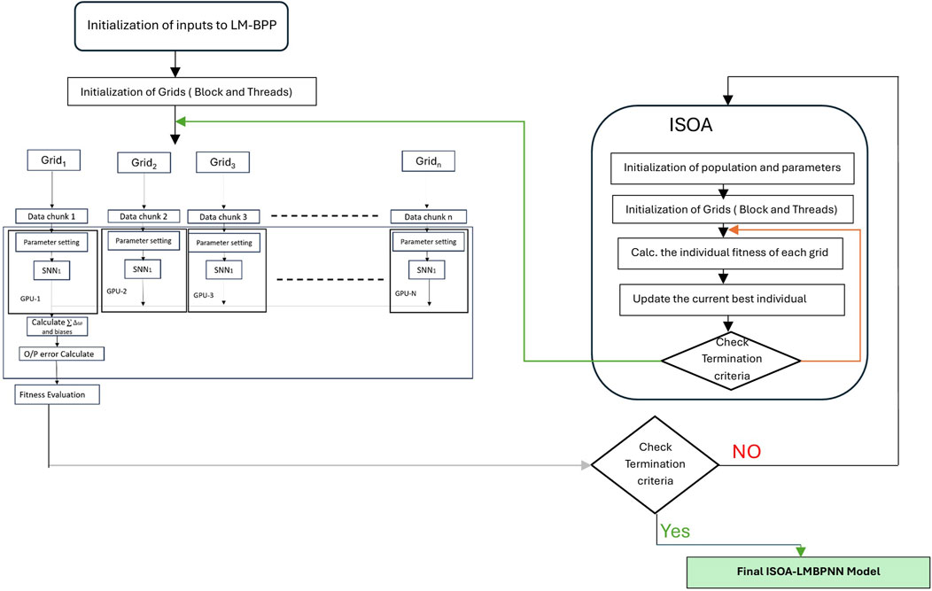
Figure 4. Block diagram of proposed ISO-LMT-BPNN flow.

Figure 5

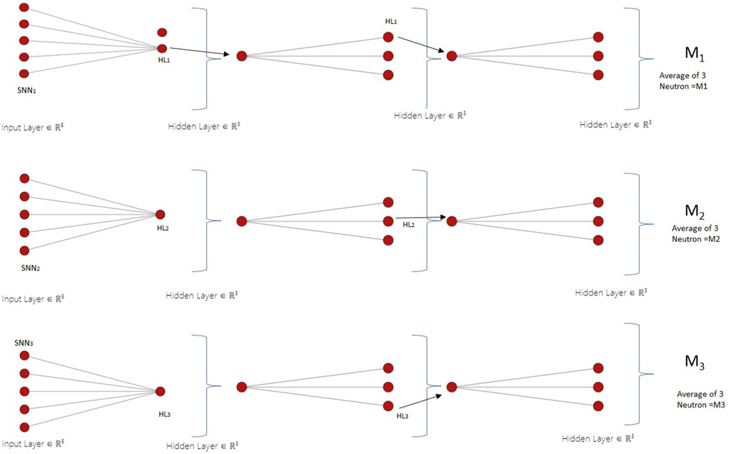
Figure 5. Neural network split into sub-neural networks (SNN_i).

Figure 6

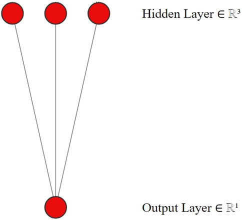
Figure 6. Output of each SNN_i merging into main neural network.

In each SNN_i, in the exploration phase, seagulls navigate the solution space, seeking optimal outcomes. The adjustment of each seagull’s position is influenced by its current location, the optimal seagull’s position within the group, and a random factor simulating the inherent exploration tendencies of seagulls. During the exploitation phase, seagulls capitalize on the best-identified solutions to discover improved results. This involves adjusting their positions around the most promising solution, aiding in the precise refinement of these solutions. Fitness values are used to rank seagulls, and for the highest-ranking among them in each SNN_i, the LM optimization technique is applied to hone the neural network’s weights and biases. This ensures minimization of training data error. After training each SNN_i, the original solutions are substituted with optimized ones. An average is calculated across SNN_i to determine if the root mean squared error (RMSE) falls below a specific threshold (10%). Conclusively, the fittest seagull will possess the optimal set of weights and biases for the CUDA-accelerated LM-BPNN.

3 Results and discussion

We now present simulated experimental data generated through a graphical user interface (GUI). The development of this interface was accomplished using the Python programming language, with PyCharm IDE serving as the primary development environment. As depicted in Figure 7, the GUI is structured to facilitate several key functionalities: it allows for the loading of datasets, provides tools for model training, and offers the capacity to produce performance metrics. Additionally, Figures 7 and 8 offer a visual comparison, illustrating the performance contrasts of the proposed model.

Figure 7

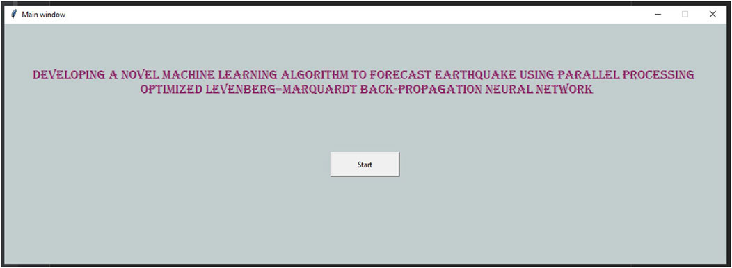
Figure 7. GUI application startup.

Figure 8

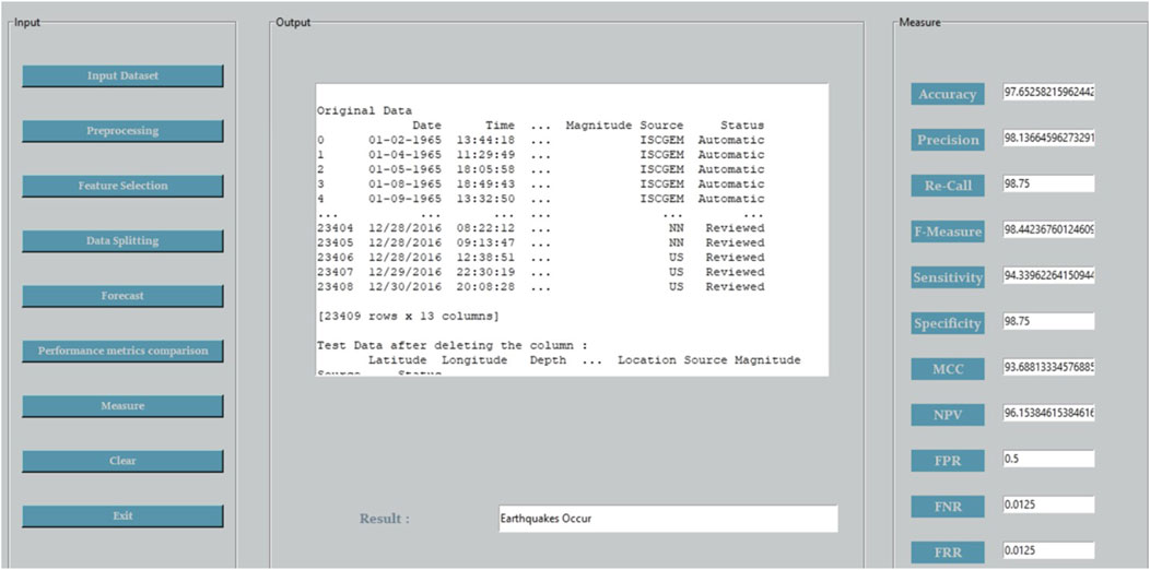
Figure 8. Analysis of various parameters and forecast results.

In Table 1, a systematic performance evaluation is presented, comparing various models against our proposed model, all tested on an earthquake dataset. From Figure 9, it becomes evident that the proposed model exhibits superior performance characteristics relative to existing models in the context of the dataset under consideration.

Table 1

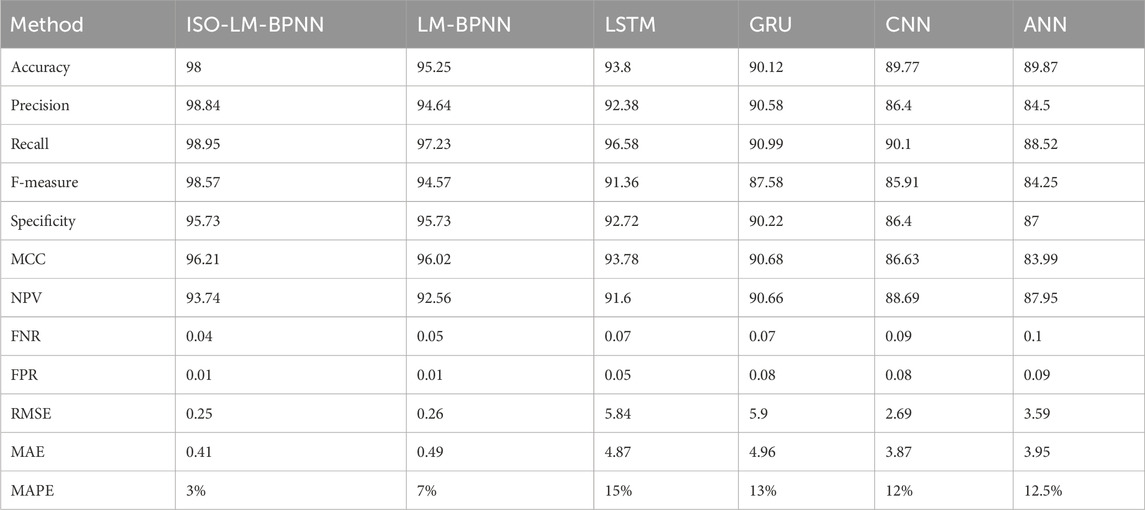
Table 1. Comparison of metrics for evaluating the effectiveness of proposed and established methods.

Figure 9

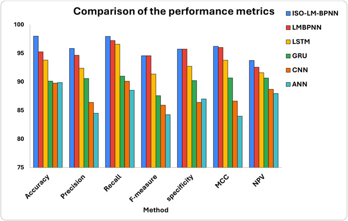
Figure 9. Comparative analysis of accuracy, precision, recall, F-measure, specificity, MCC, and NPV for proposed and existing approaches.

From the analysis presented in Figure 10, the mean absolute percentage error (MAPE) for the proposed model stands at a mere 3%. Reference to Table 2 establishes a benchmark wherein a MAPE value less than 10% signifies a superior predictive model. Given that the LMBNN model also yields a MAPE value below this 10% threshold, it can be inferred that it possesses commendable predictive capabilities. While other models evaluated in this study report MAPE values under 20%—which is still acceptable for certain applications—it is evident that the ISO-LMBPNN model boasts a notably higher prediction accuracy.

Figure 10

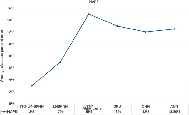
Figure 10. MAPE analysis result of ISO-LMT-BPNN with existing methods.

Table 2

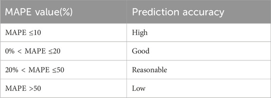
Table 2. MAPE values for prediction accuracy.

Analyzing Figure 11, it is apparent that the convergence rates of all evaluated models are strikingly similar. This close alignment can be attributed to the modest size of the dataset, leading to rapid convergence across all models. However, as the size of the dataset and its inherent complexity escalate, the convergence dynamics of the algorithms shift. In contexts such as traffic flow prediction and an earthquake database, a discernible distinction emerges. The proposed ISO-LMBPNN model demonstrates superior performance, as can be further evidenced by Figures 12 and 13, relative to the other models under consideration.

Figure 11

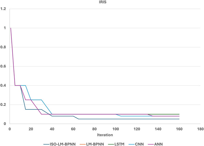
Figure 11. Convergence rate of models for Iris database.

Figure 12

Figure 12. Convergence rate of models for traffic-flow prediction.

Figure 13

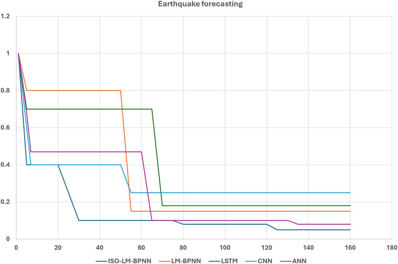
Figure 13. Convergence rate of models for earthquake database.

In this study, we assess and compare the throughput across three types of parallelism: data, model, and hybrid. “Throughput” is defined as the number of training samples processed every second. To ensure the integrity and consistency of our findings, the throughput metrics were gathered during a specific window of training, from the initial (0^th) to the 160^th iterations. These values were derived from evaluations on distinct platforms: a single CPU, TB1, and TB2. For implementing data parallelism, we utilized the PyTorch framework; model parallelism was achieved using Caffe; for hybrid parallelism, a custom CUDA kernel was crafted and employed.

Note: TB1- 1050Ti GPU and TB2 - 2 RTX 2080TI with NVLink.

Reference to Table 3 reveals that the throughput for the ISO-LMBPNN on a CPU exhibits a marked 33% improvement over the existing LMBNN. A closer examination of parallelism strategies suggests that data parallelism outpaces model parallelism; this is because of staleness mitigation (C.-C. Chen, Yang, and Cheng, 2019). However, the introduction of hybrid parallelism addresses this limitation. Indeed, the proposed model’s throughput surpasses both data and model parallelism by a notable margin of 10%.

Table 3

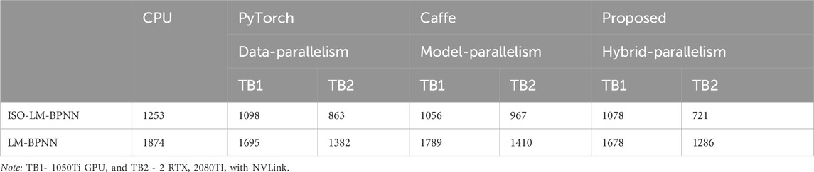
Table 3. Performance breakdown of data, model, and hybrid parallelism to an earthquake dataset with their computing time in seconds(S).

An evaluation of the performance dynamics between ISO-LM-BPNN and LM-BPNN across three diverse datasets underscores the pivotal role that both the size and intricacy of a database play in influencing computational speed.

Figure 14 describes the performance dynamics of the proposed model in comparison with LM-BPNN, specifically when applied to the Iris database. A careful examination of Figure 14 reveals a parity in computational speeds between CPU and GPU for both ISO-LMT-BPNN and LM-BPNN across all tested scenarios. This observed uniformity can be attributed to the modest size of the dataset, characterized by a limited number of instances. Consequently, the anticipated advantages of GPU utilization were not realized. The processes of dataset loading, offloading, and the allocation of grids and threads collectively contributed to equivalent execution times across all GPU platforms.

Figure 14

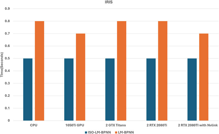
Figure 14. Performance of CPU vs. GPUs for Iris dataset.

Upon analyzing Figure 15, it becomes evident that the proposed model exhibits a substantial 72% performance differential. In contrast, the existing LMBNN model demonstrates a 50% disparity when comparing computational results from a CPU against those from a configuration of two RTX 2080Ti GPUs interconnected via NVLink.

Figure 15

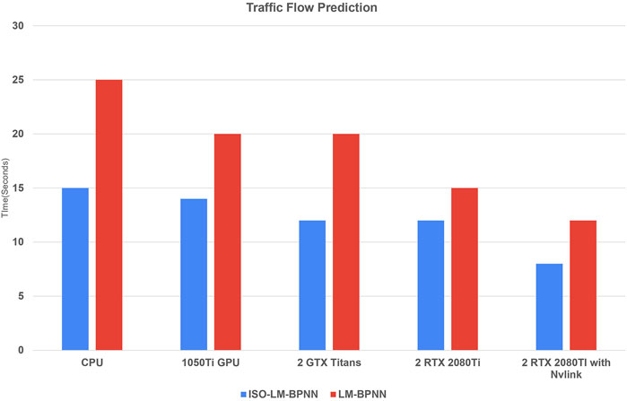
Figure 15. Performance of model with various CPU and GPUs approach for traffic-flow database.

Figure 16 illustrates a direct relationship between the intricacy and magnitude of the database and the model’s performance metrics. Specifically, when juxtaposing results from a CPU with those from a singular 1050Ti GPU, a performance uptick of 15% is observed. In a parallel comparison against a configuration of two RTX 2080Ti GPUs interconnected via NVLink, the performance surge reaches 54%. This pattern underscores the efficacy of employing robust GPU configurations in amplifying computational processes. From these observations, one can infer that the model not only scales efficiently but is also adeptly tailored for GPU-oriented operations.

Figure 16

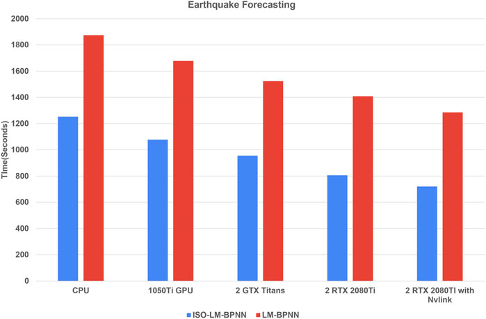
Figure 16. Performance of model with various CPU and GPUs approach for earthquake database.

4 Conclusions

In this study, we devised the ISO algorithm with the aim of refining the precision of the Levenberg–Marquardt backpropagation neural network, particularly in the realm of earthquake forecasting. The model’s accuracy fundamentally hinges on the apt identification of neural network parameters. Given the extensive computational demands associated with training deep neural networks, leveraging GPU acceleration has emerged as an effective strategy for augmenting computational velocity. Evaluations of the ISO-CUDA-accelerated LM-BPPNN were conducted across three distinct datasets and juxtaposed against four pre-existing algorithms. The findings indicate a remarkable 98% model accuracy achieved through the proposed approach. Furthermore, a computational enhancement of 40% was realized by embracing hybrid parallelism, thereby sidestepping the inherent obstacles present in both data and model parallelism. BPNN across all tested scenarios. This observed uniformity can be attributed to the modest size of the dataset, characterized by a limited number of instances. Consequently, the anticipated advantages of GPU.

Data availability statement

The raw data supporting the conclusions of this article will be made available by the authors, without undue reservation.

Author contributions

MK: Conceptualization, Data curation, Formal Analysis, Investigation, Methodology, Validation, Visualization, Writing–original draft, Writing–review and editing. AJ: Supervision, Validation, Writing–review and editing.

Funding

The author(s) declare that financial support was received for the research, authorship, and/or publication of this article. The author(s) would like to acknowledge that the publication charges for this article were funded by Department of Electrical and computer Engineering and The university of West Indies. We are grateful for their financial support, which has enabled the dissemination of our research.

Acknowledgments

We are grateful to Prof. Sanjay Bahadoorsingh for their invaluable guidance, unwavering support, and insightful feedback throughout the research process. We are also grateful to the University of West Indies, St. Augustine for providing access to essential resources that facilitated this study.

Conflict of interest

The authors declare that the research was conducted in the absence of any commercial or financial relationships that could be construed as a potential conflict of interest.

Publisher’s note

All claims expressed in this article are solely those of the authors and do not necessarily represent those of their affiliated organizations, or those of the publisher, the editors and the reviewers. Any product that may be evaluated in this article, or claim that may be made by its manufacturer, is not guaranteed or endorsed by the publisher.

References

Amin, M., Kashif, M., Sarwar, M., Rehman, A., Waheed, F., and Rehman, H. (2019). Parallel backpropagation neural network training techniques using Graphics processing unit. Int. J. Adv. Comput. Sci. Appl. 10. doi:10.14569/ijacsa.2019.0100270

CrossRef Full Text | Google Scholar

Anandhan, M., Sarepaka, R. G. V., and Hariharan, P. (2013). Prediction of surface roughness using artificial neural network in single point diamond turning. Int. J. Sci. Res. 2 (5). doi:10.36106/IJSR

CrossRef Full Text | Google Scholar

Asim, K. M., Moustafa, S. S. R., Azim Niaz, I., Elawadi, E. A., Iqbal, T., and Martínez-Álvarez, F. (2020). Seismicity analysis and machine learning models for short-term low magnitude seismic activity predictions in Cyprus. Soil Dyn. Earthq. Eng. 130, 105932. doi:10.1016/j.soildyn.2019.105932

CrossRef Full Text | Google Scholar

Aslam, B., Zafar, A., Khalil, U., and Azam, U. (2021). Seismic activity prediction of the northern part of Pakistan from novel machine learning technique. J. Seismol. 25 (2), 639–652. doi:10.1007/s10950-021-09982-3

CrossRef Full Text | Google Scholar

Bandala, A., Nakano, R. C. S., and Faelden, G. E. U. (2015). “Implementation of an artificial neural network in recognizing in-flight quadrotor images,” in 2015 IEEE region 10 conference (TENCON 2015).

CrossRef Full Text | Google Scholar

Bergstra, J., and Bengio, Y. (2012). Random search for hyper-parameter optimization. J. Mach. Learn. Res. 13, 281–305. doi:10.5555/2188385.2188395

CrossRef Full Text | Google Scholar

Chatterjee, A., Gupta, U., Kumar Chinnakotla, M., Srikanth, R., Galley, M., and Agrawal, P. (2019). Understanding emotions in text using deep learning and big data. Comput. Hum. Behav. 93, 309–317. doi:10.1016/j.chb.2018.12.029

CrossRef Full Text | Google Scholar

Chen, C.-C., Yang, C.-L., and Cheng, H.-Y. (2019). Efficient and robust parallel dnn training through model parallelism on multi-gpu platform. arXiv. arxiv.org/pdf/1809.02839.pdf.

Google Scholar

Cui, S., Yin, Y., Wang, D., Li, Z., and Wang, Y. (2021). A stacking-based ensemble learning method for earthquake casualty prediction. Appl. Soft Comput. 101, 107038. doi:10.1016/j.asoc.2020.107038

CrossRef Full Text | Google Scholar

Danielsson, J., Jagemar, M., Behnam, M., Sjodin, M., and Seceleanu, T. (2018). “Measurement-based evaluation of data-parallelism for OpenCV feature-detection algorithms,” in 2018 IEEE 42nd annual computer software and applications conference (COMPSAC).

CrossRef Full Text | Google Scholar

Dhiman, G., and Kumar, V. (2019). Seagull optimization algorithm: theory and its applications for large-scale industrial engineering problems. Knowl. Based Syst. 165, 169–196. doi:10.1016/j.knosys.2018.11.024

CrossRef Full Text | Google Scholar

Fisher, R. A. (1988). Iris. UCI machine learning repository.

Google Scholar

Florido, E., Asencio–Cortés, G., Aznarte, J. L., Rubio-Escudero, C., and Martínez–Álvarez, F. (2018). A novel tree-based algorithm to discover seismic patterns in earthquake catalogs. Comput. and Geosciences 115, 96–104. doi:10.1016/j.cageo.2018.03.005

CrossRef Full Text | Google Scholar

Ghorpade-Aher, J., Parande, J., Kulkarni, M., and Bawaskar, A. (2012). GPGPU processing in CUDA architecture.

Google Scholar

Gitis, V. G., and Derendyaev, A. B. (2019). Machine learning methods for seismic hazards forecast. Geosciences 9 (7), 308. doi:10.3390/geosciences9070308

CrossRef Full Text | Google Scholar

Jasper, S., Hugo, L., and Adams Ryan, P. (2012). Practical bayesian optimization of machine learning algorithms.

Google Scholar

Jena, R., Pradhan, B., Beydoun, G., Alamri, A. M., Ardiansyah, N., Sofyan, H., et al. (2020). Earthquake hazard and risk assessment using machine learning approaches at Palu, Indonesia. Sci. Total Environ. 749, 141582. doi:10.1016/j.scitotenv.2020.141582

PubMed Abstract | CrossRef Full Text | Google Scholar

Khan, S. U., Islam, N., Jan, Z., Din, I.Ud, and Rodrigues, J. J. P. C. (2019). A novel deep learning based framework for the detection and classification of breast cancer using transfer learning. Pattern Recognit. Lett. 125, 1–6. doi:10.1016/j.patrec.2019.03.022

CrossRef Full Text | Google Scholar

Kollam, M., and Joshi, A. (2020). “Earthquake forecasting by parallel support vector regression using CUDA,” in 2020 international conference on computing, electronics and communications engineering (iCCECE) (Southend, UK).

CrossRef Full Text | Google Scholar

Lin, J.-W., Chao, C.-T., and Chiou, J.-S. (2018). Backpropagation neural network as earthquake early warning tool using a new modified elementary Levenberg–Marquardt Algorithm to minimise backpropagation errors. Geoscientific Instrum. Methods Data Syst. 7 (3), 235–243. doi:10.5194/gi-7-235-2018

CrossRef Full Text | Google Scholar

López-Martínez, M., Díaz-Flórez, G., Villagrana-Barraza, S., Solís-Sánchez, L. O., Guerrero-Osuna, H. A., Soto-Zarazúa, G. M., et al. (2023). A high-performance computing cluster for distributed deep learning: a practical case of weed classification using convolutional neural network models. Appl. Sci. 13 (10), 6007. doi:10.3390/app13106007

CrossRef Full Text | Google Scholar

Mousavi, S. M., and Beroza, G. C. (2020). A machine-learning approach for earthquake magnitude estimation. Geophys. Res. Lett. 47 (1). doi:10.1029/2019gl085976

CrossRef Full Text | Google Scholar

Murata, N., Yoshizawa, S., and Amari, S. (1994). Network information criterion-determining the number of hidden units for an artificial neural network model. Trans. Neur. Netw. 5 (6), 865–872. doi:10.1109/72.329683

PubMed Abstract | CrossRef Full Text | Google Scholar

Nibha, M., and Burris, J. W. (2019). “An application of image classification to saltwater fish identification in Louisiana fisheries,” in 3rd international conference on information system and data mining.

Google Scholar

Ragab, M., Alshehri, S., Alhakamy, N. A., Alsaggaf, W., Alhadrami, H. A., and Alyami, J. (2022). Machine learning with quantum seagull optimization model for COVID-19 chest X-ray image classification. J. Healthc. Eng. 2022, 1–13. doi:10.1155/2022/6074538

CrossRef Full Text | Google Scholar

Rao, D. T. V. D., and Ramana, K. V. (2019). Accelerating training of deep neural networks on GPU using CUDA. Int. J. Intelligent Syst. Appl. 11 (5), 18–26. doi:10.5815/ijisa.2019.05.03

CrossRef Full Text | Google Scholar

Ravanelli, M., Zhong, J., Pascual, S., Swietojanski, P., Monteiro, J., Trmal, J., et al. (2020). “Multi-task self-supervised learning for robust speech recognition,” in IEEE international conference on acoustics, speech and signal processing (ICASSP).

CrossRef Full Text | Google Scholar

Rundle, J., Donnellan, A., Fox, G., Crutchfield, J., and Granat, R. (2021). Nowcasting earthquakes: imaging the earthquake cycle in California with machine learning. Earth Space Sci. 8. doi:10.1029/2021EA001757

CrossRef Full Text | Google Scholar

Sanders, J., and Kandrot, E. (2010). CUDA by example: an introduction to general-purpose GPU programming. 1 ed. Addison-Wesley Professional.

Google Scholar

Singh, S., Paul, A., and Arun, M. (2017). “Parallelization of digit recognition system using deep convolutional neural network on CUDA,” in Sensing, signal processing and security (ICSSS), 2017 third international conference.

CrossRef Full Text | Google Scholar

U.S.Geological Survey (2020). Earthquake lists, maps, and statistics. Available at: https://www.usgs.gov/natural-hazards/earthquake-hazards/lists-maps-and-statistics.

Google Scholar

Venkata Divya, U., and Sai Prasad, P. S. V. S. (2018). Hashing supported iterative MapReduce based scalable SBE reduct computation. Distributed Comput. Internet Technol. Cham, 163–170. doi:10.1007/978-3-319-72344-0_13

CrossRef Full Text | Google Scholar

Xiong, P., Long, C., Zhou, H., Battiston, R., Zhang, X., and Shen, X. (2020). Identification of electromagnetic pre-earthquake perturbations from the DEMETER data by machine learning. Remote Sens. 12 (21), 3643. doi:10.3390/rs12213643

CrossRef Full Text | Google Scholar

Xiong, P., Tong, L., Zhang, K., Shen, X., Battiston, R., Ouzounov, D., et al. (2021). Towards advancing the earthquake forecasting by machine learning of satellite data. Sci. Total Environ. 771, 145256. doi:10.1016/j.scitotenv.2021.145256

PubMed Abstract | CrossRef Full Text | Google Scholar

Zhang, Q., Zhang, M., Chen, T., Sun, Z., Ma, Y., and Yu, B. (2018). Recent advances in convolutional neural network acceleration. Neurocomputing 323, 37–51. doi:10.1016/j.neucom.2018.09.038

CrossRef Full Text | Google Scholar

Zhao, L. (2021). “Traffic flow forecasting,” in Webology: UCI machine learning repository.

Google Scholar

Zhou, R., Wu, D., Fang, L., Xu, A., and Lou, X. (2018). A levenberg–marquardt backpropagation neural network for predicting forest growing stock based on the least-squares equation fitting parameters. Forests 9 (12), 757. doi:10.3390/f9120757

CrossRef Full Text | Google Scholar

Zukovic, M., Borovsky, M., Lach, M. ´uˇs, and Hristopulos, D. T. (2020). GPU-Accelerated simulation of massive spatial data based on the modified planar rotator model. Math. Geosci. 52 (1), 123–143. doi:10.1007/s11004-019-09835-3

CrossRef Full Text | Google Scholar