Method for estimating tension of two Nielsen–Lohse bridge cables with intersection clamp connection and unknown boundary conditions

Nielsen–Lohse bridges are tied arch bridges with inclined cables that cross each other and connect through intersection clamps. Estimating the tension acting on the cables is essential for maintenance. Currently, methods for estimating the tension of a single cable using natural frequencies are applied to each cable after removing the intersection clamps. However, the removal and re-installation of intersection clamps is time-consuming and laborious. To improve the efficiency of tension estimation, the authors previously proposed a method for simultaneously estimating the tension of two cables with an attached intersection clamp. However, the previous method has the drawback of considering simple support at both ends, even though the actual boundary is not a perfect simple support. The objective of this study is to develop a new method for estimating the tension of two cables with unknown boundary conditions. The cable is assumed to be supported by a rotational spring at both ends. The newly proposed method estimates the tension, bending stiffness, and rotational stiffness of two cables from the natural frequencies without requiring the removal of the intersection clamp. The proposed method can handle arbitrary boundary conditions such as simple support or fixed support. In the case of fixed support, the rotational spring constant becomes infinity. To avoid infinity in the computation, normalization was employed in the derivation of the estimation formula. The validity of the proposed method was verified by numerical simulations and field experiments on an actual Nielsen–Lohse bridge. In the field experiment, the tension of all eight cables was accurately estimated and the estimation error was less than 10%. Even when accelerometers were installed on only one of the two cables at a height near the girder, the tension of both cables was estimated with good accuracy. The proposed method improves the efficiency of tension estimation work, because the tension of two cables can be estimated simultaneously and with good accuracy by measuring the acceleration of only one cable at a height near the girder.

1 Introduction

In cable-supported bridges, cables play an important role in supporting the load of structures. Because each cable has its own load capacity, it is necessary to carry out maintenance work so as to ensure that the tension acting on the cable is lower than the cable’s load capacity. The cable tension can be measured directly using a load cell, but direct measurement is disadvantageous in terms of cost. Therefore, the cable tension is typically estimated indirectly from the cable’s natural frequencies.

In Japan, the vibration method of Shinke et al. (1980) and Zui et al. (1996) and the higher-order vibration method of Yamagiwa et al. (2000) are often used to estimate the tension of a single cable. The vibration method (Shinke et al., 1980; Zui et al., 1996) estimates the cable tension by inputting the first- or second-mode natural frequency and two parameters accounting for the cable’s bending stiffness, sag, and inclination angle. Therefore, the bending stiffness must be pre-evaluated. In practice, however, the bending stiffness is often unknown, which makes pre-evaluation difficult. The higher-order vibration method (Yamagiwa et al., 2000) solves this problem by estimating the tension and bending stiffness simultaneously from the natural frequencies under simple support and fixed support conditions, without requiring the pre-evaluation of bending stiffness. Fang and Wang (2012) proposed an estimation formula similar to the higher-order vibration method (Yamagiwa et al., 2000). Their formula simultaneously estimates the tension and bending stiffness of a cable with fixed end boundaries. Additionally, they recommend using a curve-fitting technique to avoid the iterative calculations required by the higher-order vibration method. Nam and Nghia (2011) derived an estimation equation that considers both the bending stiffness and sag of the cable.

The complex boundary conditions of cables have also been investigated. Utsuno et al. (1998) assumed that the cable is supported by a rotational spring at both ends, and proposed a method for estimating the cable’s tension, bending moment, and rotational stiffness using the higher-order vibration method. Ma (2017) proposed a method for estimating the tension of an inclined cable with unknown boundary conditions from the natural frequencies. Yan et al. (2019) proposed a method for estimating cable tension; their method handles arbitrary boundaries by using mode shapes. Ma (2017) and Yan et al. (2019) modeled arbitrary boundaries using rotational springs. Furukawa et al. (2021, 2022a, 2022b, 2023) proposed methods for estimating the tension of a cable with a damper installed near the cable boundary from the natural frequencies and mode shapes. A damper is directly modeled with complex stiffness, and a formula has been proposed to estimate the tension, bending stiffness, and damper parameters simultaneously from the natural frequencies. Chen et al. (2016, 2018) and Wu et al. (2018) proposed novel tension estimation methods for handling asymmetric and complex boundary conditions by using mode shapes. Their methods avoid the direct modeling of complex boundaries by focusing on cable deflections at locations away from the cable boundaries with the help of mode shapes.

Although the above-mentioned methods can estimate the cable tension under arbitrary boundary conditions, these tension estimation methods consider a single cable.

The present study considered the Nielsen–Lohse bridge type, which is an arch bridge characterized by two diagonal cables connected by an intersection clamp, as shown in Figure 1. Intersection clamps are installed to prevent the damage and noise caused by the contact between cables. Owing to the diagonal cables, Nielsen–Lohse bridges have less deflection and horizontal vibrations compared with normal arch bridges (Sakano et al., 2003). Owing to the vortex-induced vibration caused by the diagonal cables, Nielsen–Lohse bridges rarely oscillate (Yoneda, 2000). The diagonal cables reduce the bending moments on the arch ribs and stiffening girders. Therefore, diagonal cables play an important role in Nielsen–Lohse bridges. Nevertheless, diagonal cables in Nielsen–Lohse bridges are prone to fatigue, and cable assessment is required.

FIGURE 1

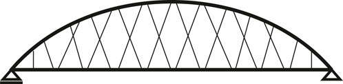
FIGURE 1. Schematic diagram of Nielsen–Lohse bridge.

Notably, in Nielsen–Lohse bridges, the cable loosens owing to seismic motion in the bridge axial direction (Sakoda et al., 2000). Therefore, the boundary conditions at both ends of the cables change. Hence, the boundary conditions must be properly handled when estimating the tension of Nielsen–Lohse bridge cables.

In the current practice of cable tension estimation for Nielsen–Lohse bridges, the vibration method (Shinke et al., 1980; Zui et al., 1996) or higher-order vibration method (Yamagiwa et al., 2000) is applied to every single cable after removing the intersection clamps. Because intersection clamps are typically installed high above the girders, their removal and re-installation requires an aerial work platform, which in turn requires traffic control. In summary, current inspection practice is time-consuming and laborious because it requires the operation of an aerial work platform and traffic control.

Few studies have attempted to estimate the cable tension of Nielsen–Lohse bridges without removing the intersection clamps. The authors are only aware of the study by Kuriyama et al. (1994), who proposed that the cable between one end and the intersection clamp can be considered as a single cable, and applied the higher-order vibration method without removing the intersection clamp. However, it is inappropriate to consider the intersection clamp as a fixed end, because the intersection clamp is not fixed and vibrates. Therefore, to the author’s knowledge, an appropriate tension estimation method for Nielsen–Lohse bridges is still lacking.

With this background, this study investigated tension estimation methods suitable to Nielsen–Lohse bridges. The authors have previously proposed two methods based on the higher-order vibration method (Furukawa et al., 2022c). The first one is the out-of-plane method, which simultaneously estimates the tension and bending stiffness of two cables from the natural frequencies in the out-of-plane direction. The second one is the in-plane method, which estimates the tension, bending stiffness, and axial stiffness of two cables simultaneously from the natural frequencies in the in-plane direction. Numerical and experimental verifications have revealed that the out-of-plane method has higher estimation accuracy compared with the in-plane method. Further experimental investigations have indicated that the accuracy of the in-plane natural frequencies is lower than the accuracy of the out-of-plane natural frequencies, which explains why the out-of-plane method is more accurate, according to experimental verifications (Furukawa et al., 2022d). Based on these findings, the out-of-plane method was selected as the most appropriate method.

The methods previously proposed by the authors have a drawback in that both ends of the cables are modeled as simply supported. However, as mentioned previously, the actual boundaries have rotational stiffness, and the boundary conditions change because the boundaries loosen. Some Nielsen–Lohse bridges employ short cables, for which the boundary conditions have a stronger effect on the natural frequencies. Therefore, it is necessary to improve the previous methods so as to appropriately handle the boundary conditions.

This paper proposes a new tension estimation method for Nielsen–Lohse bridges with unknown boundary conditions. The proposed method assumes that the cables are supported by rotational springs at the cable ends. The simple support condition corresponds to a rotational spring constant equal to zero, and the fixed support condition corresponds to a rotational spring constant equal to infinity. The proposed method estimates the tension, bending stiffness, and rotational stiffness of two cables simultaneously using the natural frequencies in the out-of-plane direction and does not require the removal of intersection clamps. Because the rotational spring constant becomes infinity in the case of fixed support, normalization is introduced into the proposed method to avoid the numerical difficulty of handing infinity. The effect of the rotational stiffness on the tension estimation accuracy of the previously proposed method was numerically investigated, and the necessity of rotational stiffness is discussed. The validity of the proposed method was verified through the numerical simulation of 42 models and field experiments on an actual bridge.

2 Proposed method for estimating cable tension

2.1 Definition of coordinate system and cable parameters

This section presents the new tension estimation method for two cables connected by an intersection clamp and supported by rotational springs, as shown in Figure 2A. The proposed method considers out-of-plane vibration perpendicular to the plane formed by the two cables.

FIGURE 2

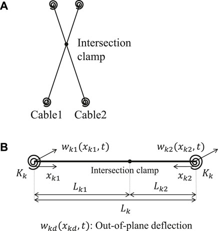
FIGURE 2. Target model. (A) Model of two cables connected by intersection clamp. (B) Direction of coordinate axes and deflection in element coordinate system.

Figure 2B shows the element coordinate system of cable $k$, where the cable number $k\left(k=\mathrm{1,2}\right)$ is given to each of the two cables. The subscript $k$ indicates the value for cable $k$. Let $L_{k1}$ and $L_{k2}$ be the cable length of the left and right sides of the intersection clamp; the total cable length $L_k$ is $L_{k1}+L_{k2}$. Next, let us introduce an index $d\left(d=\mathrm{1,2}\right)$ representing the left and right sides (spans) of the intersection clamp. Let the cable axis be $x_{kd}$ and the out-of-plane deflection of position $x_{kd}$ at time $t$ be $w_{kd}\left(x_{kd},t\right)$, as shown in Figure 2B. Notably, axes $x_{k1}$ and $x_{k2}$ are taken in the opposite direction.

The other cable parameters are defined as follows: $T_k$ is the tension, $E_k{I}_k$ is the bending stiffness ($E_k$: Young’s modulus, $I_k$: second moment of area), ${\rho }_k{A}_k$ is the mass per unit length (${\rho }_k$: density, $A_k$: area), and $K_k$ is the rotational spring constant of cable $k$; $T_k$, $E_k{I}_k$, ${\rho }_k$, and $A_k$ are uniform throughout the same cable. Each cable $k$ has rotational springs with the same spring constant $K_k$ at both ends. This study develops a tension estimation method using natural frequencies. Considering that the effect of damping on the natural frequencies is small, damping at the boundaries is neglected.

2.2 Governing equation and general solution of cable deflection

The out-of-plane deflection $w_{kd}\left(x_{kd},t\right)$ of the cable position $x_{kd}$ at time $t$ for cable $k$ follows the following governing equation when the cable is considered as a tensioned Euler–Bernoulli beam:

${\rho }_k{A}_k\frac{{\partial }^2{w}_{kd}\left(x_{kd},t\right)}{\partial t^2}+E_k{I}_k\frac{{\partial }^4{w}_{kd}\left(x_{kd},t\right)}{\partial x_{kd}^4}-T_k\frac{{\partial }^2{w}_{kd}\left(x_{kd},t\right)}{\partial x_{kd}^2}=0,(1)$

The deflection is transformed by variable separation, as follows:

$w_{kd}\left(x_{kd},t\right)=W_{kd}\left(x_{kd}\right)\exp \left(j\omega t\right)(2)$

where $W_{kd}\left(x_{kd}\right)$ is the modal function for position $x_{kd}$, $j$ is an imaginary unit, and $\omega$ is the angular frequency. By substituting Eq. 2 into Eq. 1, the general solution of $W_{kd}\left(x_{kd}\right)$ can be obtained as follows:

$W_{kd}\left(x_{kd}\right)=C_{kd1}\cos {\alpha }_k{x}_{kd}+C_{kd2}\sin {\alpha }_k{x}_{kd}+C_{kd3}\cosh {\beta }_k{x}_{kd}+C_{kd4}\sinh {\beta }_k{x}_{kd},(3)$

where $C_{kd1}$, $C_{kd2}$, $C_{kd3}$, and $C_{kd4}$ are the integration constants, and ${\alpha }_k$ and ${\beta }_k$ are expressed as follows:

${\alpha }_k=\sqrt{\sqrt{{\left(\frac{T_k}{2E_k{I}_k}\right)}^2+\frac{{\rho }_k{A}_k{\omega }^2}{E_k{I}_k}}-\frac{T_k}{2E_k{I}_k}},(4)$

${\beta }_k=\sqrt{\sqrt{{\left(\frac{T_k}{2E_k{I}_k}\right)}^2+\frac{{\rho }_k{A}_k{\omega }^2}{E_k{I}_k}}+\frac{T_k}{2E_k{I}_k}}.(5)$

Because there are 16 integration constants ($C_{kd1}$, $C_{kd2}$, $C_{kd3}$, and $C_{kd4}$ for $k=1,2$ and $d=1,2$), 16 boundary conditions are required.

2.3 Boundary conditions

The following equations hold for each cable at each end, when the cable is supported by a rotational spring:

$W_{kd}\left(0\right)=0,(6)$

$\frac{d^2{W}_{kd}\left(0\right)}{d{x}_{kd}^2}=P_k\frac{d{W}_{kd}\left(0\right)}{d{x}_{kd}},(7)$

where $P_k$ is expressed as follows:

$P_k=\frac{K_k}{E_k{I}_k}.(8)$

For each cable, the continuity conditions of the deflection, deflection angle, and curvature on both sides of the intersection clamp are expressed as follows:

$W_{k1}\left(L_{k1}\right)=W_{k2}\left(L_{k2}\right),(9)$

$\frac{d{W}_{k1}\left(L_k\right)}{d{x}_{k1}}+\frac{d{W}_{k2}\left(L_{k2}\right)}{d{x}_{k2}}=0,(10)$

$\frac{d^2{W}_{k1}\left(L_{k1}\right)}{d{x}_{k1}^2}=\frac{d^2{W}_{k2}\left(L_{k2}\right)}{d{x}_{k2}^2}.(11)$

Because the out-of-plane deflections of the two cables are equal at the intersection clamp, the following equation holds:

$W_{12}\left(L_{12}\right)=W_{22}\left(L_{22}\right).(12)$

The two cables interact with the force of each other. Because the forces on each cable are equal in magnitude and opposite in direction at the intersection clamp, the following boundary condition can be established:

$\begin{array}{l}{E}_1{I}_1\left\{\frac{d^3{W}_{11}\left(L_{11}\right)}{d{x}_{11}^3}+\frac{d^3{W}_{12}\left(L_{12}\right)}{d{x}_{12}^3}\right\}+T_1\left\{\frac{d{W}_{11}\left(L_{11}\right)}{d{x}_{11}}+\frac{d{W}_{12}\left(L_{12}\right)}{d{x}_{12}}\right\}\\ +E_2{I}_2\left\{\frac{d^3{W}_{21}\left(L_{21}\right)}{d{x}_{21}^3}+\frac{d^3{W}_{22}\left(L_{22}\right)}{d{x}_{22}^3}\right\}+T_2\left\{\frac{d{W}_{21}\left(L_{21}\right)}{d{x}_{21}}+\frac{d{W}_{22}\left(L_{22}\right)}{d{x}_{22}}\right\}=0.\end{array}(13)$

Thus far, 16 boundary conditions have been developed, that is, Eqs 6, 7 for each cable at each end (eight boundary conditions), Eqs 9–11 for each cable (six boundary conditions), and Eqs 12, 13 (two boundary conditions).

2.4 Substituting general solution of cable deflection into boundary conditions

Next, the general solution in Eq. 3 is substituted into the boundary conditions.

First, by substituting Eq. 3 into Eqs 6, 7 and writing the resulting equation in matrix format, the following equation is obtained:

$\left[\begin{array}{cc}1& 1\\ -{\alpha }_k^2& {\beta }_k^2\end{array}\right]\left\{\begin{array}{c}{C}_{kd1}\\ C_{kd3}\end{array}\right\}=P_k\left[\begin{array}{cc}0& 0\\ {\alpha }_k& {\beta }_k\end{array}\right]\left\{\begin{array}{c}{C}_{kd2}\\ C_{kd4}\end{array}\right\}.(14)$

Hence, ${\left\{C_{kd1}{C}_{kd3}\right\}}^T$ can be expressed by ${\left\{C_{kd2}{C}_{kd4}\right\}}^T$, as follows:

$\left\{\begin{array}{c}{C}_{kd1}\\ C_{kd3}\end{array}\right\}=\frac{P_k}{{\alpha }_k^2+{\beta }_k^2}\left[\begin{array}{cc}-{\alpha }_k& -{\beta }_k\\ {\alpha }_k& {\beta }_k\end{array}\right]\left\{\begin{array}{c}{C}_{kd2}\\ C_{kd4}\end{array}\right\}.(15)$

Then, by substituting Eq. 15 into Eq. 3 and substituting $L_{kd}$ into $x_{kd}$, ${\left\{W_{kd}\left(L_{kd}\right)d^2{W}_{kd}\left(L_{kd}\right)/d{x}_{kd}^2\right\}}^T$ can be expressed using the 2 × 2 matrix ${\mathit{Q}}_{kd}$ and ${\left\{C_{kd2}{C}_{kd4}\right\}}^T$ as follows:

$\begin{array}{l}\left\{\begin{array}{c}{W}_{kd}\left(L_{kd}\right)\\ \frac{d^2{W}_{kd}\left(L_{kd}\right)}{d{x}_{kd}^2}\end{array}\right\}=\left[\begin{array}{cc}\sin {\alpha }_k{L}_{kd}& \sinh {\beta }_k{L}_{kd}\\ -{\alpha }_k^2\sin {\alpha }_k{L}_{kd}& {\beta }_k^2\sinh {\beta }_k{L}_{kd}\end{array}\right]\left\{\begin{array}{c}{C}_{kd2}\\ C_{kd4}\end{array}\right\}+\left[\begin{array}{cc}\cos {\alpha }_k{L}_{kd}& \cosh {\beta }_k{L}_{kd}\\ -{\alpha }_k^2\cos {\alpha }_k{L}_{kd}& {\beta }_k^2\cosh {\beta }_k{L}_{kd}\end{array}\right]\left\{\begin{array}{c}{C}_{kd1}\\ C_{kd3}\end{array}\right\}\\ =\left\{\left[\begin{array}{cc}\sin {\alpha }_k{L}_{kd}& \sinh {\beta }_k{L}_{kd}\\ -{\alpha }_k^2\sin {\alpha }_k{x}_{kd}& {\beta }_k^2\sinh {\beta }_k{L}_{kd}\end{array}\right]+\frac{P_k}{{\alpha }_k^2+{\beta }_k^2}\left[\begin{array}{cc}\cos {\alpha }_k{L}_{kd}& \cosh {\beta }_k{L}_{kd}\\ -{\alpha }_k^2\cos {\alpha }_k{L}_{kd}& {\beta }_k^2\cosh {\beta }_k{L}_{kd}\end{array}\right]\left[\begin{array}{cc}-{\alpha }_k& -{\beta }_k\\ {\alpha }_k& {\beta }_k\end{array}\right]\right\}\left\{\begin{array}{c}{C}_{kd2}\\ C_{kd4}\end{array}\right\}\\ ={\mathit{Q}}_{kd}\left\{\begin{array}{c}{C}_{kd2}\\ C_{kd4}\end{array}\right\},\end{array}(\mathrm{16a})$

where

${\mathit{Q}}_{kd}=\left[\begin{array}{cc}\sin {\alpha }_k{L}_{kd}& \sinh {\beta }_k{L}_{kd}\\ -{\alpha }_k^2\sin {\alpha }_k{x}_{kd}& {\beta }_k^2\sinh {\beta }_k{L}_{kd}\end{array}\right]+\frac{P_k}{{\alpha }_k^2+{\beta }_k^2}\left[\begin{array}{cc}\cos {\alpha }_k{L}_{kd}& \cosh {\beta }_k{L}_{kd}\\ -{\alpha }_k^2\cos {\alpha }_k{L}_{kd}& {\beta }_k^2\cosh {\beta }_k{L}_{kd}\end{array}\right]\left[\begin{array}{cc}-{\alpha }_k& -{\beta }_k\\ {\alpha }_k& {\beta }_k\end{array}\right].(\mathrm{16b})$

By substituting Eq.16a into Eqs 9, 11, the following expression is obtained:

${\mathit{Q}}_{k1}\left\{\begin{array}{c}{C}_{k12}\\ C_{k14}\end{array}\right\}={\mathit{Q}}_{k2}\left\{\begin{array}{c}{C}_{k22}\\ C_{k24}\end{array}\right\}.(17)$

From the above analysis, ${\left\{C_{k12}{C}_{k14}\right\}}^T$ can be expressed by the 2 × 2 matrix ${\mathit{Q}}_k$ and ${\left\{C_{k22}{C}_{k24}\right\}}^T$ as follows:

$\left\{\begin{array}{c}{C}_{k12}\\ C_{k14}\end{array}\right\}={\mathit{Q}}_{k1}^{-1}{\mathit{Q}}_{k2}\left\{\begin{array}{c}{C}_{k22}\\ C_{k24}\end{array}\right\}={\mathit{Q}}_k\left\{\begin{array}{c}{C}_{k22}\\ C_{k24}\end{array}\right\},(\mathrm{18a})$

where

${\mathit{Q}}_k={\mathit{Q}}_{k1}^{-1}{\mathit{Q}}_{k2}(\mathrm{18b})$

Next, by substituting Eq. 15 into Eq. 3 and substituting $L_{kd}$ into $x_{kd}$, $d{W}_{kd}\left(L_{kd}\right)/d{x}_{kd}$ can be expressed using the 1 × 2 matrix ${\mathit{R}}_{kd}$ and ${\left\{C_{kd2}{C}_{kd4}\right\}}^T$, as follows:

$\begin{array}{l}\frac{d{W}_{kd}\left(L_{kd}\right)}{d{x}_{kd}}=\left[\begin{array}{cc}{\alpha }_k\cos {\alpha }_k{L}_{kd}& {\beta }_k\cosh {\beta }_k{L}_{kd}\end{array}\right]\left\{\begin{array}{c}{C}_{kd2}\\ C_{kd4}\end{array}\right\}+\left[-\begin{array}{cc}{\alpha }_k\sin {\alpha }_k{L}_{kd}& {\beta }_k\sinh {\beta }_k{L}_{kd}\end{array}\right]\left\{\begin{array}{c}{C}_{kd1}\\ C_{kd3}\end{array}\right\}\\ =\left\{\left[\begin{array}{cc}{\alpha }_k\cos {\alpha }_k{L}_{kd}& {\beta }_k\cosh {\beta }_k{L}_{kd}\end{array}\right]+\frac{P_k}{{\alpha }_k^2+{\beta }_k^2}\left[-\begin{array}{cc}{\alpha }_k\sin {\alpha }_k{L}_{kd}& {\beta }_k\sinh {\beta }_k{L}_{kd}\end{array}\right]\left[\begin{array}{cc}-{\alpha }_k& -{\beta }_k\\ {\alpha }_k& {\beta }_k\end{array}\right]\right\}\left\{\begin{array}{c}{C}_{kd2}\\ C_{kd4}\end{array}\right\}\\ ={\mathit{R}}_{kd}\left\{\begin{array}{c}{C}_{kd2}\\ C_{kd4}\end{array}\right\},\end{array}(\mathrm{19a})$

where

${\mathit{R}}_{kd}=\left[\begin{array}{cc}{\alpha }_k\cos {\alpha }_k{L}_{kd}& {\beta }_k\cosh {\beta }_k{L}_{kd}\end{array}\right]+\frac{P_k}{{\alpha }_k^2+{\beta }_k^2}\left[-\begin{array}{cc}{\alpha }_k\sin {\alpha }_k{L}_{kd}& {\beta }_k\sinh {\beta }_k{L}_{kd}\end{array}\right]\left[\begin{array}{cc}-{\alpha }_k& -{\beta }_k\\ {\alpha }_k& {\beta }_k\end{array}\right](\mathrm{19b})$

By substituting Eq. 19a into Eq. 10 and using Eq 18a, 18 the following equation is obtained:

${\mathit{R}}_{k1}\left\{\begin{array}{c}{C}_{k12}\\ C_{k14}\end{array}\right\}+{\mathit{R}}_{k2}\left\{\begin{array}{c}{C}_{k22}\\ C_{k24}\end{array}\right\}=\left[{\mathit{R}}_{k1}{\mathit{Q}}_k+{\mathit{R}}_{k2}\right]\left\{\begin{array}{c}{C}_{k22}\\ C_{k24}\end{array}\right\}={\mathit{S}}_k\left\{\begin{array}{c}{C}_{k22}\\ C_{k24}\end{array}\right\}=0,(\mathrm{20a})$

where ${\mathit{S}}_k$ is a 1 × 2 matrix expressed as follows:

${\mathit{S}}_k={\mathit{R}}_{k1}{\mathit{Q}}_k+{\mathit{R}}_{k2}(\mathrm{20b})$

Then, Eq. 20a can be transformed as follows:

$C_{k24}=-\frac{S_k\left(\mathrm{1,1}\right)}{S_k\left(\mathrm{1,2}\right)}{C}_{k22}(21)$

where $S_k\left(\mathrm{1,1}\right)$ and $S_k\left(\mathrm{1,2}\right)$ are the (1,1)-th and (1,2)-th entries of matrix ${\mathit{S}}_k\left(k=\mathrm{1,2}\right)$.

Next, by substituting Eq. 16a into Eq. 12, the following equation is obtained:

$Q_{12}\left(\mathrm{1,1}\right)C_{122}+Q_{12}\left(\mathrm{1,2}\right)C_{124}=Q_{22}\left(\mathrm{1,1}\right)C_{222}+Q_{22}\left(\mathrm{1,2}\right)C_{224}(22)$

where $Q_{k2}\left(\mathrm{1,1}\right)$ and $Q_{k2}\left(\mathrm{1,2}\right)$ are the (1,1)-th and (1,2)-th entries of matrix ${\mathit{Q}}_{k2}$ ($k=\mathrm{1,2}$).

By substituting Eq. 21 into Eq. 22, the following equation is obtained:

$\left(Q_{12}\left(\mathrm{1,1}\right)-Q_{12}\left(\mathrm{1,2}\right)\frac{S_1\left(\mathrm{1,1}\right)}{S_1\left(\mathrm{1,2}\right)}\right)C_{122}=\left(Q_{22}\left(\mathrm{1,1}\right)-Q_{22}\left(\mathrm{1,2}\right)\frac{S_2\left(\mathrm{1,1}\right)}{S_2\left(\mathrm{1,2}\right)}\right)C_{222}(23)$

Next, by substituting Eq. 15 into Eq. 3 and substituting $L_{kd}$ into $x_{kd}$, $d^3{W}_{kd}\left(L_{kd}\right)/d{x}_{kd}^3$ can be expressed using the 1 × 2 matrix ${\mathit{T}}_{kd}$ and ${\left\{C_{kd2}{C}_{kd4}\right\}}^T$, as follows:

$\begin{array}{l}\frac{d^3{W}_{kd}\left(L_{kd}\right)}{d{x}_{kd}^3}=\left[\begin{array}{cc}-{\alpha }_k^3\cos {\alpha }_k{L}_{kd}& {\beta }_k^3\cosh {\beta }_k{L}_{kd}\end{array}\right]\left\{\begin{array}{c}{C}_{kd2}\\ C_{kd4}\end{array}\right\}+\left[\begin{array}{cc}{\alpha }_k^3\sin {\alpha }_k{L}_{kd}& {\beta }_k^3\sinh {\beta }_k{L}_{kd}\end{array}\right]\left\{\begin{array}{c}{C}_{kd1}\\ C_{kd3}\end{array}\right\}\\ =\left\{\left[\begin{array}{cc}-{\alpha }_k^3\cos {\alpha }_k{L}_{kd}& {\beta }_k^3\cosh {\beta }_k{L}_{kd}\end{array}\right]+\frac{P_k}{{\alpha }_k^2+{\beta }_k^2}\left[\begin{array}{cc}{\alpha }_k^3\sin {\alpha }_k{L}_{kd}& {\beta }_k^3\sinh {\beta }_k{L}_{kd}\end{array}\right]\left[\begin{array}{cc}-{\alpha }_k& -{\beta }_k\\ {\alpha }_k& {\beta }_k\end{array}\right]\right\}\left\{\begin{array}{c}{C}_{kd2}\\ C_{kd4}\end{array}\right\}\\ ={\mathit{T}}_{kd}\left\{\begin{array}{c}{C}_{kd2}\\ C_{kd4}\end{array}\right\},\end{array}(\mathrm{24a})$

where

${\mathit{T}}_{kd}=\left[\begin{array}{cc}-{\alpha }_k^3\cos {\alpha }_k{L}_{kd}& {\beta }_k^3\cosh {\beta }_k{L}_{kd}\end{array}\right]+\frac{P_k}{{\alpha }_k^3+{\beta }_k^3}\left[\begin{array}{cc}{\alpha }_k^3\sin {\alpha }_k{L}_{kd}& {\beta }_k^3\sinh {\beta }_k{L}_{kd}\end{array}\right]\left[\begin{array}{cc}-{\alpha }_k& -{\beta }_k\\ {\alpha }_k& {\beta }_k\end{array}\right](\mathrm{24b})$

Hence, the following equation is obtained:

$\frac{d^3{W}_{k1}\left(L_{k1}\right)}{d{x}_{k1}^3}+\frac{d^3{W}_{k2}\left(L_{k2}\right)}{d{x}_{k2}^3}={\mathit{T}}_{k1}\left\{\begin{array}{c}{C}_{k12}\\ C_{k14}\end{array}\right\}+{\mathit{T}}_{k2}\left\{\begin{array}{c}{C}_{k22}\\ C_{k24}\end{array}\right\}=\left[{\mathit{T}}_{k1}{\mathit{Q}}_k+{\mathit{T}}_{k2}\right]\left\{\begin{array}{c}{C}_{k22}\\ C_{k24}\end{array}\right\}={\mathit{U}}_k\left\{\begin{array}{c}{C}_{k22}\\ C_{k24}\end{array}\right\},(\mathrm{25a})$

where ${\mathit{U}}_k$ is a 1 × 2 matrix expressed as follows: ${\mathit{U}}_k={\mathit{T}}_{k1}{\mathit{Q}}_k+{\mathit{T}}_{k2}\mathrm{(25b)}$

By substituting Eqs 10, 25a into Eq. 13, the following equation is obtained:

$E_1{I}_1{\mathit{U}}_1\left\{\begin{array}{c}{C}_{122}\\ C_{124}\end{array}\right\}+E_2{I}_2{\mathit{U}}_2\left\{\begin{array}{c}{C}_{222}\\ C_{224}\end{array}\right\}=0.(26)$

By substituting Eq. 21 into Eq. 26 and dividing by $E_2{I}_2$, the following equation is obtained:

$\frac{E_1{I}_1}{E_2{I}_2}\left(U_1\left(\mathrm{1,1}\right)-U_1\left(\mathrm{1,2}\right)\frac{S_1\left(\mathrm{1,1}\right)}{S_1\left(\mathrm{1,2}\right)}\right)C_{122}+\left(U_2\left(\mathrm{1,1}\right)-U_2\left(\mathrm{1,2}\right)\frac{S_2\left(\mathrm{1,1}\right)}{S_2\left(\mathrm{1,2}\right)}\right)C_{222}=0(27)$

where $U_k\left(\mathrm{1,1}\right)$ and $U_k\left(\mathrm{1,2}\right)$ are the (1,1)-th and (1,2)-th entries of matrix ${\mathit{U}}_k$ ($k=\mathrm{1,2}$).

By combining Eq. 23 and 27, the following equation is obtained:

$\left[\begin{array}{cc}{a}_1& -a_2\\ E_1{I}_1{b}_1& E_2{I}_2{b}_2\end{array}\right]\left\{\begin{array}{c}{C}_{122}\\ C_{222}\end{array}\right\}=\left\{\begin{array}{c}0\\ 0\end{array}\right\}(28)$

where $a_k$ and $b_k$ are expressed as follows:

$a_k=Q_{k2}\left(\mathrm{1,1}\right)-Q_{k2}\left(\mathrm{1,2}\right)\frac{S_k\left(\mathrm{1,1}\right)}{S_k\left(\mathrm{1,2}\right)}(29)$

$b_k=U_k\left(\mathrm{1,1}\right)-U_k\left(\mathrm{1,2}\right)\frac{S_k\left(\mathrm{1,1}\right)}{S_k\left(\mathrm{1,2}\right)}(30)$

Notably, $a_k$ and $b_k$ comprise only functions related to cable $k$ and do not include functions related to the other cable.

If $C_{122}$ and $C_{222}$ are both equal to zero, all integral constants become zero, as expressed by Eqs 15, 18a, 21. Therefore, for the mode function $W_{kd}\left(x_{kd}\right)$ to have a nontrivial solution, the determinant of the matrix in Eq. 28 must be zero. Finally, the following constraint equation is derived:

$\frac{E_1{I}_1}{E_2{I}_2}{b}_1{a}_2+b_2{a}_1=0.(31)$

2.5 Constraint equation for natural frequencies

There are infinitely many natural frequencies that satisfy Eq. 31. Let $i$ be a positive integer and $f_i$ be the corresponding natural frequency. Then, Eq. 31 can be rewritten as follows:

$\frac{E_1{I}_1}{E_2{I}_2}{b}_1^i{a}_2^i+b_2^i{a}_1^i=0.(32)$

The superscript $i$ indicates the value for the $i$^th mode; $a_k^i$ and $b_k^i$ are functions related to $T_k$, $E_k{I}_k$, ${\rho }_k{A}_k$, $L_k$, $L_{kd}$, and $r_k$ of cable $k$, and the $i$^th natural frequency $f_i$. The natural frequency $f_i$ is not explicitly included in functions $a_k^i$ and $b_k^i$, but is included in ${\alpha }_k^i$ and ${\beta }_k^i$, as follows:

${\alpha }_k^i=\sqrt{\sqrt{{\left(\frac{T_k}{2E_k{I}_k}\right)}^2+\frac{{\rho }_k{A}_k{\left(2\pi f_i\right)}^2}{E_k{I}_k}}-\frac{T_k}{2E_k{I}_k}}(33)$

${\beta }_k^i=\sqrt{\sqrt{{\left(\frac{T_k}{2E_k{I}_k}\right)}^2+\frac{{\rho }_k{A}_k{\left(2\pi f_i\right)}^2}{E_k{I}_k}}+\frac{T_k}{2E_k{I}_k}}(34)$

Thus far, it is clear from the expression expansion that $a_k^i$ and $b_k^i$ are functions depending on $P_k$. In the case of fixed support, $a_k^i$ and $b_k^i$ become infinity because $P_k$ becomes infinity. Therefore, it is difficult to precisely calculate Eq. 32 in the case of fixed support.

To solve this problem, Eq. 32 is normalized with regard to $P_k$, as follows:

$G^i\equiv \left(\frac{E_1{I}_1}{E_2{I}_2}\frac{b_1^i}{a_1^i}+\frac{b_2^i}{a_2^i}\right)·\frac{a_1^i}{\mathit{max}\left(\left|a_1^1\right|,\left|a_1^i\right|\right)}·\frac{a_2^i}{\mathit{max}\left(\left|a_2^1\right|,\left|a_2^i\right|\right)}=0;(35)$

where $b_k^i$ is normalized by division with $a_k^i$, and $a_k^i$ is normalized by division with $\mathit{max}\left(\left|a_k^1\right|,\left|a_k^i\right|\right)$.

By organizing the formulas, it can be found that $b_k^i/a_k^i$ and $a_k^i/\mathit{max}\left(\left|a_k^1\right|,\left|a_k^1\right|\right)$ can be expressed as the ratio of two cubic functions of $P_k$. Therefore, $b_k^i/a_k^i$ and $a_k^i/\mathit{max}\left(\left|a_k^1\right|,\left|a_k^i\right|\right)$ can be calculated using the different formulas expressed by Eqs 36, 37 depending on the rotational stiffness $r_k$ ($0\le r_k\le 1$) defined in Eq. 38.

$\frac{b_k^i}{a_k^i}=\{\begin{array}{c}\frac{{\sum }_{m=0}^3{b}_{km}^i·P_k^m}{{\sum }_{m=0}^3{a}_{km}^i·P_k^m}\left(r_k<1\right)\\ \frac{b_{k3}^i}{a_{k3}^i}\left(r_k=1\right)\end{array}(36)$

$\frac{a_k^i}{\mathit{max}\left(\left|a_k^1\right|,\left|a_k^i\right|\right)}=\{\begin{array}{c}\frac{{\sum }_{m=0}^3{a}_{km}^i·P_k^m}{\mathit{max}\left(\left|{\sum }_{m=0}^3{a}_{km}^1·P_k^m\right|,\left|{\sum }_{m=0}^3{a}_{km}^i·P_k^m\right|\right)}\left(r_k<1\right)\\ \frac{a_{k3}^i}{\mathit{max}\left(\left|a_{k3}^1\right|,\left|a_{k3}^i\right|\right)}\left(r_k=1\right)\end{array}(37)$

$r_k=\frac{K_k{L}_k}{{\pi }^4{E}_k{I}_k+K_k{L}_k}=\frac{P_k{L}_k/{\pi }^4}{1+P_k{L}_k/{\pi }^4}.(38)$

where $a_{km}^i$ and $b_{km}^i$ ($m=\mathrm{0,1,2,3}$) are coefficients of $P_k^m$ and are related to cable $k$ and mode $i$; $r_k=0$ represents simple support ($K_k=P_k=0$) and $r_k=1$ represents fixed support ($K_k=P_k=\infty$). Thus, the computation of infinite values when $P_k$ becomes infinity is avoided. This study assumes that the bending stiffness and the rotational springs are in series, but the bending and rotational stiffness can be estimated independently because they are independent in Eqs 35–37. The rotational stiffness is only included in $P_k$, and the bending stiffness is included in $a_{km}^i$, $b_{km}^i$, and $P_k$ in Eqs 36, 37.

2.6 Procedure of cable tension estimation

The proposed method estimates the tension $T_k$, bending stiffness $E_k{I}_k$, and rotational stiffness $r_k$ of two cables simultaneously by solving the following optimization problem:

$minimizeG\left(T_1,T_2,E_1{I}_1,E_2{I}_2,r_1,r_2\right)={\displaystyle \sum }_{i=1}^n{\left(G^i\right)}^2,(39)$

where $G$ is the objective function to be minimized, $G^i$ is the function defined in Eq. 35, and $n$ is the total number of natural frequencies used in the estimation. The mass per unit length ${\rho }_k{A}_k$, cable length $L_k$, position of intersection clamp $L_{kd}$, and measured natural frequencies $f_i$ must be input into Eq. 39. Because there are six unknowns, namely, the tension $T_k$, bending stiffness $E_k{I}_k$, and rotational stiffness $r_k$ of the two cables, more than six natural frequencies are needed. The proposed method also estimates the bending and rotational stiffness, but the estimation accuracy is not satisfactory owing to these properties’ low sensitivity, as will be explained later.

Because Eq. 39 is a nonlinear least-squares problem, the MultiStart method was adopted (MathWorks, 2020) to avoid a local minima solution. In the MultiStart method, the solution (combination of $T_1,T_2,E_1{I}_1,E_2{I}_2,r_1,$ and $r_2$) that minimizes the objective function $G$ is estimated from various initial values of $T_1,T_2,E_1{I}_1,E_2{I}_2,r_1,$ and $r_2$. Among the various solutions based on various initial values, the solution with the minimum objective function is determined as the globally optimal solution.

$G^i$ is normalized with regard to $P_k$ as shown in Eqs 35–37. $G^i$ is not perfectly normalized for all functions, but is found to be of approximately similar magnitude for different $i$.

2.7 Previously proposed method assuming simple support

The previously proposed out-of-plane method (Furukawa et al., 2022c) assumes that both ends of the two cables have simple support, and estimates the tension $T_k$ and bending stiffness $E_k{I}_k$ of the two cables from the natural frequencies in the out-of-plane direction. The optimization problem of the previously proposed method is expressed as follows:

$minimize{G}_{pre}\left(T_1,T_2,E_1{I}_1,E_2{I}_2\right)={\displaystyle \sum }_{i=1}^n{\left(G_{pre}^i\right)}^2,(40)$

where $G_{pre}$ is the objective function to be minimized, $G_{pre}^i$ is the function defined in Eq. 41, and $n$ is the total number of natural frequencies used in the estimation.

$G_{pre}^i=\sin {\alpha }_1^i{L}_1{g}_2^i+\frac{E_2{I}_2}{E_1{I}_1}\frac{{\left({\alpha }_2^i\right)}^3+{\alpha }_2^i{\left({\beta }_2^i\right)}^2}{{\left({\alpha }_1^i\right)}^3+{\alpha }_1^i{\left({\beta }_1^i\right)}^2}\sin {\alpha }_2^i{L}_2{g}_1^i(41)$

where

$g_k^i=\sin {\alpha }_k^i{L}_{k1}\sin {\alpha }_k^i{L}_{k2}-\frac{{\alpha }_k^i}{{\beta }_k^i}\sin {\alpha }_k^i{L}_k\frac{1+e^{-2{\beta }_k^i{L}_k}-e^{-2{\beta }_k^i{L}_{k1}}-e^{-2{\beta }_k^i{L}_{k2}}}{2\left(1-e^{-2{\beta }_k^i{L}_k}\right)}.(42)$

Notably, Eq. 41 does not exactly match Eq. 35, even if $P_k$ is substituted with zero, because the formulae are organized differently.

3 Numerical verification

3.1 Overview

This section discusses the numerical validation of the proposed method. The tension, bending stiffness, and rotational stiffness of the two cables were estimated using the natural frequencies in the out-of-plane direction, which were obtained by the eigenvalue analysis of the finite element method. The estimation accuracy was investigated by comparing the estimated value to the assumed (true) value.

3.2 Modeling of two cables with intersection clamp

The material properties, length, and intersection clamp locations of actual Nielsen–Lohse bridge cables vary. Therefore, to cover a wide range of cable parameters, this study considered the various cases listed in Table 1. In Case 1, the length and material properties of the two cables are identical. In Case 2, the two cables have equal length, but their material properties are different. In Case 3, the length and material properties of the two cables are identical, but the intersection clamp location differs from model to model. In Case 4, the material properties of the two cables are equal, but the cables have different length. There are four types of cables, that is, A, B, C, and D, with different tension, bending stiffness, and mass per unit length, as presented in Table 2. A total of 42 models are listed in Table 3. Model Nos. 1–6, 7–12, 13–24, and 25–42 belong to cases 1, 2, 3, and 4, respectively.

TABLE 1

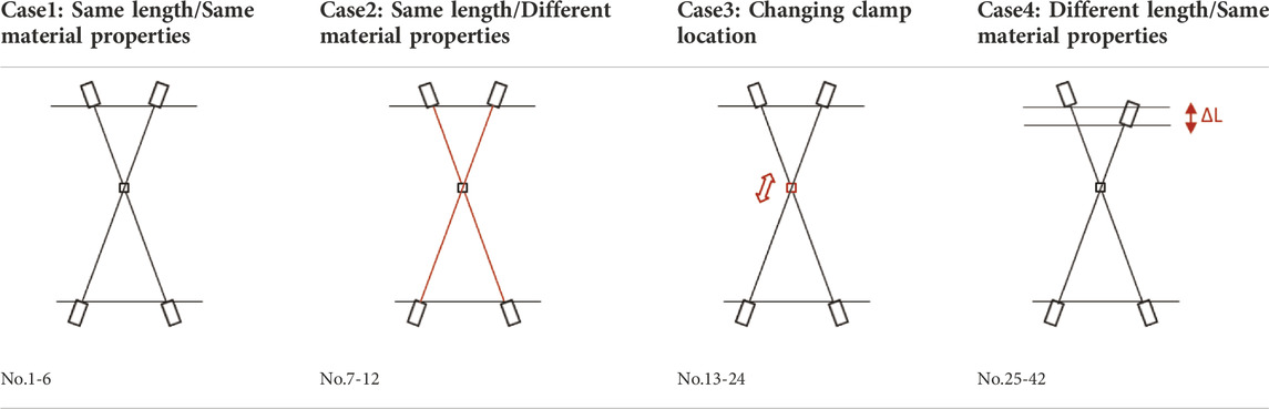
TABLE 1. Four numerical verification cases.

TABLE 2

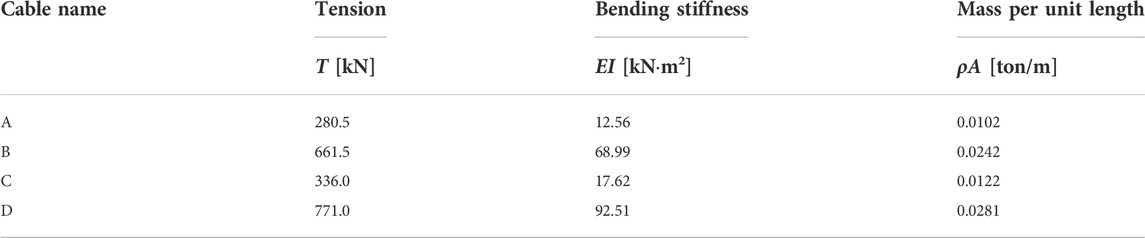
TABLE 2. Cable specifications in numerical verifications.

TABLE 3

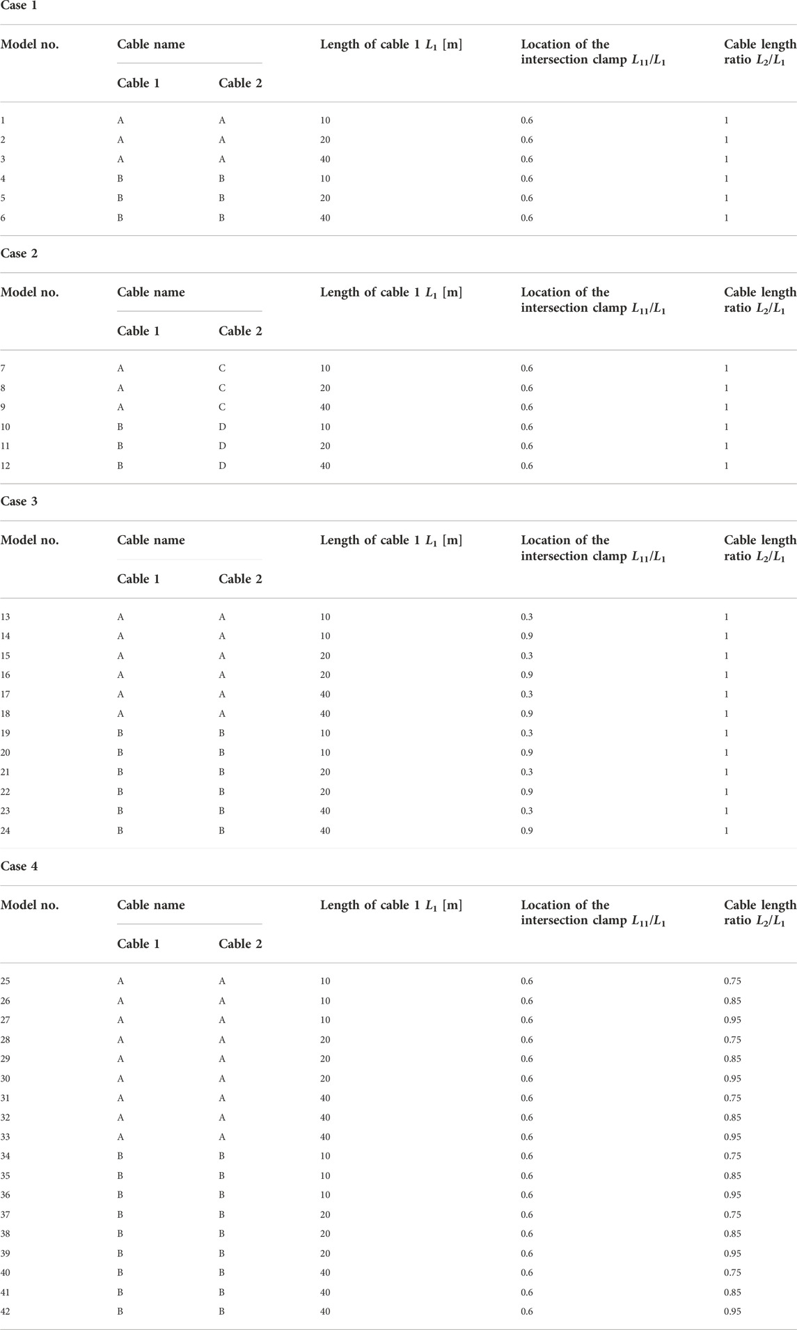
TABLE 3. Models of two cables with intersection clamp considered in numerical verifications.

3.3 Calculation of natural frequencies using finite element method

The natural frequencies of the two-cable models were obtained by the eigenvalue analysis of the finite element method. The two-dimensional analysis models for the out-of-plane deflection were established. The element size was set to 0.1 m to achieve sufficient accuracy in the calculation of the natural frequencies. Rotational springs were set at both ends of the two cables, and the deflections were fixed at both ends of the two cables.

The natural frequencies calculated by eigenvalue analysis were input into the optimization problem expressed by Eq. 39. Because there are six unknowns (the tension, bending stiffness, and rotational stiffness of the cables), the natural frequencies up to the ninth mode were used for estimation. Yamagiwa et al. (Yamagiwa et al., 2000) proposed using the lowest five modes for accurate tension estimation by the higher-order vibration method with two unknowns, because tension is sensitive to the lower natural frequencies. Because there were six unknowns in this study, nine natural frequencies were used.

3.4 Analysis conditions in solution of optimization problem

To solve the optimization problem of Eq. 39 using the MultiStart method, 1,000 sets of initial values were generated. Generally, more sets of initial values result in higher estimation accuracy but also increase the computation time. It has been confirmed that the estimation accuracy does not improve substantially even if the number of initial value sets exceeds 1,000.

The search range of the solution must be defined when solving the optimization problem. The search range of tension was set to 0.5–2 times the true value. As described in the previous study (Furukawa et al., 2022c), the objective function has local minima solutions in the range where the tension is smaller than 0.25 times the true value because the objective function does not depend on the mode order of the natural frequencies. While this has the advantage that it is not necessary to specify the mode order of the natural frequencies to be input to the objective function, the problem of local minimum solution exists. However, previous studies (Furukawa et al., 2022c) have shown that local minimum solutions can be avoided by setting the search range of tension to be greater than 0.25 times the true value. Therefore, in this study, the lower bound of the search range for tension was set to 0.5 times the true value. Harada et al. (2002) reported that the ratio of the actual tension to the design value of a Nielsen–Lohse bridge after 30 years of service is 0.76–1.4. Therefore, it is reasonable to set the search range of the tension to 0.5–2 times the true value. In this section, the search range of the bending stiffness is considered to be 0.26–2 times the true value. The search range of the rotational stiffness was set from 0 (simple support) to 1 (fixed support).

3.5 Comparison between tension estimation results obtained by newly proposed method and previously proposed method under variable rotational stiffness

Before presenting the estimation results obtained by the proposed method for 42 models, the tension estimation accuracy of the newly proposed method is compared to that of the previously proposed method.

The dimensions of the two cables are as follows: $T_1$ = 1,650 kN, $T_2$ = 3,300 kN, $E_1{I}_1=E_2{I}_2$ = 106 kN/m², ${\rho }_1{A}_1={\rho }_2{A}_2$ = 0.03 ton/m. Five cable lengths were considered: $L_1=L_2$ = 10, 20, 30, 40, 50 m. The intersection clamp position was set to $L_{11}/L_1=L_{21}/L_2$ = 0.6. Seven rotational stiffness cases were considered: $r_1=r_2$ = 0.0 (simple support), and 0.05, 0.1, 0.2, 0.5, 0.8, 1.0 (fixed support). The natural frequencies of the first nine modes without measurement error were input to both the newly proposed method and previously proposed method.

The tension estimation results are shown in Figure 3. The horizontal axis indicates the rotational stiffness for each cable length, and the vertical axis indicates the ratio of the estimated tension to the true value. When the rotational stiffness was zero, both methods estimated the tension with high accuracy. However, as the rotational stiffness increased, the estimation accuracy of the previously proposed method decreased, particularly for short cables, because the previous method assumes that both ends are simply supported, and the rotational stiffness has stronger influence on the natural frequencies of short cables. Considering a cable with a length of 10 m and fixed support, the tension estimation error is approximately 10% when the previously proposed method is used. In contrast, the newly proposed method estimates the tension with high accuracy regardless of the rotational stiffness and cable length.

FIGURE 3

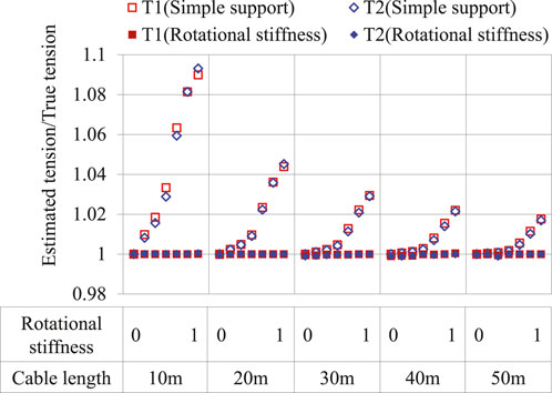
FIGURE 3. Comparison between tension estimation results of proposed method (rotational stiffness) and previously proposed method (simple support).

Based on the above comparison, it was thought necessary to consider the rotational stiffness, particularly for short cables. The proposed method considering the rotational stiffness is very useful, because there are many Nielsen–Lohse bridges with short cables (length of approximately 10–20 m).

3.6 Estimation results for tension, bending stiffness, and rotational stiffness when measurement error is ignored

First, the estimation for 42 models without measurement error was investigated. The results obtained for the case wherein the rotational stiffness of the two cables was 1 ($r_1=r_2=1$) are shown as an example.

Figure 4 shows the estimation results for the tension, bending stiffness, and rotational stiffness. The horizontal axis is the model number, and the vertical axis is the ratio of the estimated value to the true value.

FIGURE 4

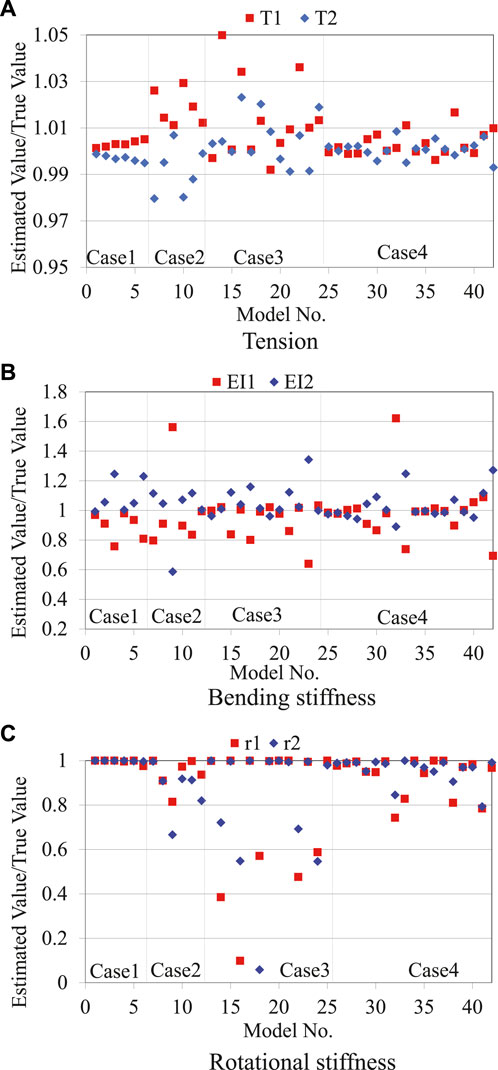
FIGURE 4. Estimation results without measurement error. (A) Tension. (B) Bending stiffness. (C) Rotational stiffness.

Figure 5 shows the sensitivity analysis results for models No. 1 and 9. As can be seen, the value of the objective function $G$ in Eq. 39 changes only when one parameter out of the six parameters (tension, bending stiffness, and rotational stiffness of the two cables) is varied. The horizontal axis gives the ratio of the value of the parameter input to the objective function to the true value, and the vertical axis gives the objective function value. The tension and bending stiffness varied from 0 to 2 times the true value. The rotational stiffness varied from 0 to 1.

FIGURE 5

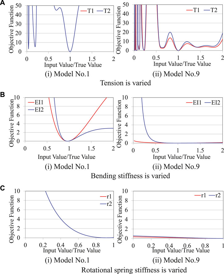
FIGURE 5. Sensitivity of tension, bending stiffness, and rotational stiffness to objective function for model No.1 (left) and model No. 9 (right). (A) Tension is varied. (B) Bending stiffness is varied. (C) Rotational spring stiffness is varied.

First, the tension estimation accuracy was investigated. As shown in Figure 4A, the proposed method estimated the tension with sufficient accuracy and the error was within 5% for all models. By carefully examining the results, it can be found that the accuracy differs depending on the model. For example, cases 1 and 4 have higher tension estimation accuracy compared with cases 2 and 3. Figure 5A shows the sensitivity analysis results for model No. 1 (case 1) and model No. 9 (case 2). The vertical axis is minimum when the horizontal axis value is 1, and rapidly increases as the horizontal axis value moves away from 1. This indicates that tension is highly sensitive to the objective function, which explains why the tension estimation accuracy is high. The vertical axis value of model No.1 exhibits greater increase compared with model No. 9. This means that the tension of model No. 1 is more sensitive to the objective function compared with that of model No. 9, which explains why the tension estimation accuracy of model No.1 is higher than that of model No. 9. The reason why local minima are observed in the range of the horizontal axis value smaller than 0.25 has already been explained in 3.4, and they can be avoided by setting the search range of the tension appropriately. Although there are differences in the estimation accuracy of each model, it can be seen that the tension estimation accuracy is generally high.

Second, the bending stiffness estimation accuracy was investigated. Based on the comparison between Figures 4A,B, the bending stiffness estimation accuracy is generally inferior to the tension estimation accuracy. In particular, the bending stiffness estimation accuracy of models No. 9 and 32 is very low, with an estimation error as high as 60%. The reason for this is that the bending stiffness has lower sensitivity against the objective function compared with tension, as determined by comparing Figures 5A,B. Particularly, the objective function of model No. 9 hardly changes even if the bending stiffness changes, as shown on the right side of Figure 5B.

This study used the natural frequencies of the first nine modes to accurately estimate the tension, because tension is sensitive to the natural frequencies of the lower modes (Yamagiwa et al., 2000). In contrast, the bending stiffness has lower sensitivity against the natural frequencies of the lower modes (Yamagiwa et al., 2000). Therefore, it is difficult to estimate the bending stiffness as accurately as tension if lower-mode natural frequencies are used.

Finally, the rotational stiffness estimation accuracy was investigated. As shown in Figure 4C, the rotational stiffness estimation accuracy is inferior to the tension estimation accuracy, because the rotational stiffness has lower sensitivity to the objective function, as can be found by comparing Figures 5A–C. The lower estimation accuracy of model No. 9, compared with model No.1, is also caused by the lower sensitivity of model No. 9, as can be found by comparing the two graphs in Figure 5C. The cable length of models No. 1 and 9 is 10 and 40 m, respectively. As shown in Figure 3, the effect of the rotational stiffness becomes smaller as the cable length increases. Because the cable is longer, the influence of the boundary conditions is smaller, and the rotational stiffness accuracy of model No. 9 is lower.

The same tendency was observed in other cases wherein a different rotational stiffness was assumed. The tension of the two cables was estimated with high accuracy and the error was less than 5%, regardless of the rotational stiffness. In contrast, the bending stiffness and rotational stiffness estimations had considerably larger errors.

3.7 Effect of measurement error on tension estimation accuracy

3.7.1 Modeling of measurement error

This section discusses the effect of measurement errors in the natural frequencies on the tension estimation accuracy.

Numerical errors are added to the $i$^th mode natural frequency $f_i^{FEM}$ calculated by the finite element method, as follows:

$f_i^{noise}=f_i^{FEM}\left(1+ϵrand\right),(43)$

where $f_i^{noise}$ is the natural frequency of the $i$^th mode with numerical error, and $rand$ is a uniform random number between -1 and 1; $ϵ$ is the error rate set to 0.0, 0.01, 0.02, 0.03, 0.04, 0.06, 0.08, and 0.1. Different random numbers are generated for each natural frequency up to the ninth mode.

3.7.2 Estimation error index

The two estimation error indices, namely, the mean absolute error ratio (MAER) and the root-mean-square error ratio (RMSER), which obtained the average degree of estimation error for all 42 models, are expressed as follows:

$MAER=\frac{1}{2N}{\displaystyle \sum }_{I=1}^N{\displaystyle \sum }_{k=1}^2\left|\frac{T_k^{noise}\left(I\right)}{T_k^{true}\left(I\right)}-1\right|,(44)$

$RMSER=\sqrt{\frac{1}{2N}{\displaystyle \sum }_{I=1}^N{\displaystyle \sum }_{k=1}^2{\left(\frac{T_k^{noise}\left(I\right)}{T_k^{true}\left(I\right)}-1\right)}^2}(45)$

where $N$ is the total number of models ($N=42$), $T_k^{true}\left(I\right)$ is the true value of tension, and $T_k^{noise}\left(I\right)$ is the tension estimated from the natural frequencies with numerical errors for cable $k$ and model No. $I$.

The tension estimation error of the higher-order vibration method has been reported to be within 5% (Shinko Wire Company, 2017). In this study, the tension estimation error target was set to be within 10%, because the proposed method deals with two connected cables, which is a considerably more difficult problem compared with dealing with a single cable. Therefore, the error rates at which the MAER and RMSER values exceed 0.1 (10%) was investigated.

3.7.3 Results

In this section, the results for the case wherein the rotational stiffness of both cables is 1 ($r_1=r_2=1$) are discussed as an example.

First, the tension of all 42 models was estimated using nine natural frequencies with measurement errors for each error rate $ϵ$ from 0.01 to 1.0. The tension estimation results for the error rate $ϵ$ = 0.01, 0.02, 0.03, and 0.05 are shown in Figure 6A as an example. As can be seen, the estimation error increases with the error rate. The estimation error indices for each error rate are shown in Figure 7A. The RMSER and MAER exceed 0.1 when the error rates exceed 0.024 and 0.02, respectively.

FIGURE 6

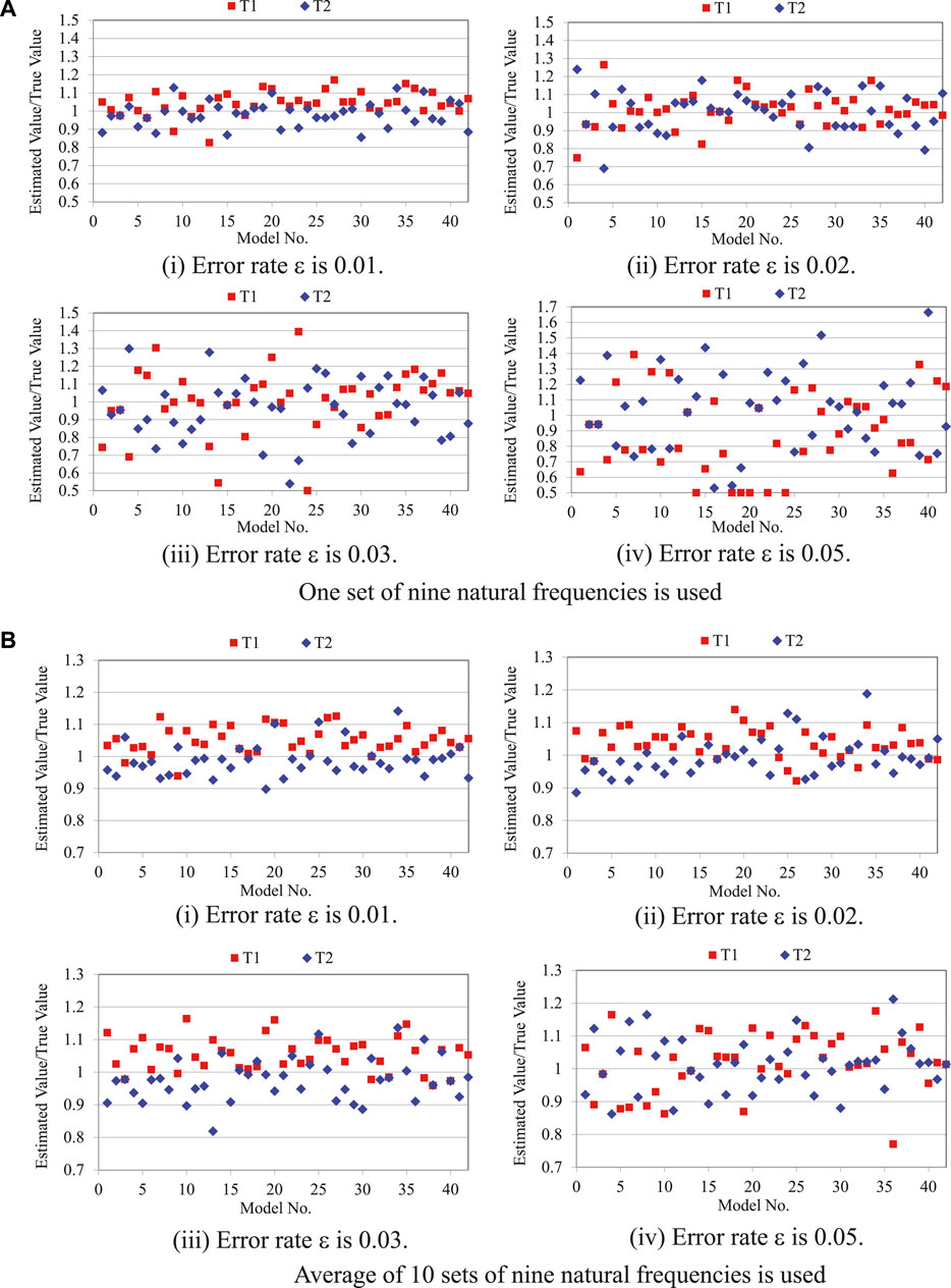
FIGURE 6. Estimation results with measurement error. (A) One set of nine natural frequencies is used. (B) Average of 10 sets of nine natural frequencies is used.

FIGURE 7

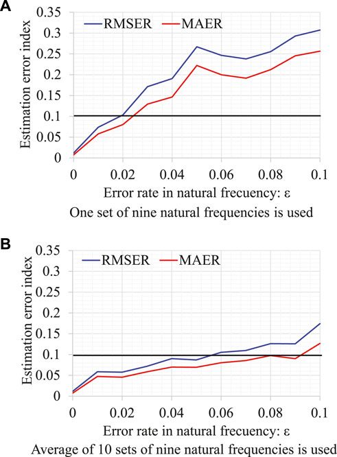
FIGURE 7. Effect of measurement errors on tension estimation error index. (A) One set of nine natural frequencies is used. (B) Average of 10 sets of nine natural frequencies is used.

Next, the average of 10 sets of nine natural frequencies was used in the estimation to reduce the effect of measurement noise. The ten sets of nine natural frequencies and the measurement error for each error rate were calculated by repeating the calculation of Eq. 43 ten times. The tension estimation results for the error rate $ϵ$ = 0.01, 0.02, 0.03, and 0.05 are shown in Figure 6B as an example. The comparison between Figures 6A,B shows that the tension estimation accuracy improved by using the average of 10 sets of nine natural frequencies. The estimation error indices for each error rate are shown in Figure 7B. The RMSER and MAER stay below 0.1 when the error rates are below 0.092 and 0.056, respectively. Therefore, using the average value of the natural frequencies obtained from multiple measurements is an effective approach for reducing the effect of measurement error on the accuracy of tension estimation.

4 Verification by field experiment on actual bridge

4.1 Outline of actual bridge experiments

A field experiment on an actual bridge was conducted to verify the validity of the proposed method. The schematic diagram of the considered Nielsen–Lohse bridge is shown in Figure 8A. Permission to use a photograph and the name of the bridge has not been obtained from the bridge administrator. In this bridge, each cable is a bundle of 19 strand steel wires covered with polyethylene coating.

FIGURE 8

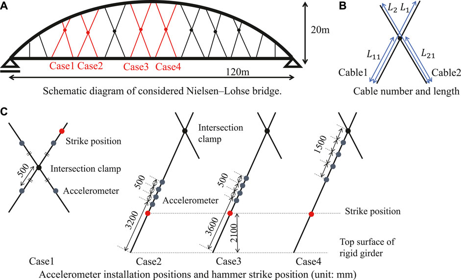
FIGURE 8. Outline of field experiment. (A) Schematic diagram of considered Nielsen–Lohse bridge. (B) Cable number and length. (C) Accelerometer installation positions and hammer strike position (unit: mm).

The vibration experiment was conducted for the four sets of two cables shown in Figure 8A, that is, cases 1, 2, 3, and 4 from the left. The cable name and length are defined in Figure 8B.

In each case, the natural frequencies were measured by four piezoelectric accelerometers. The sampling time interval is 0.00078125 s, the sampling rate is 1,280 Hz, the measurement time is 25.6 s, and the frequency resolution is 0.0390625 Hz. The accelerometers’ location and the location where the cable was hit by a hammer are shown in Figure 8C. In case 1, two accelerometers were placed on each cable near the intersection clamp. The position near the intersection clamp of cable 1 was hit with a hammer to excite vibration. In cases 2, 3, and 4, four accelerometers were placed on cable 1, and no accelerometers were placed on cable 2. The position near the bottom end of cable 1 was hit with a hammer to excite vibration. In cases 1 and 4, four accelerometers were placed high above the girder. In cases 2 and 3, four accelerometers were placed near the girder at a height reachable by ladder.

4.2 Structural specifications of each cable

The structural specifications of each cable are shown in Table 4. Case 1 has the shortest cable length, and case 4 has the longest cable length. The values in the “Design document” column were obtained from the design document.

TABLE 4

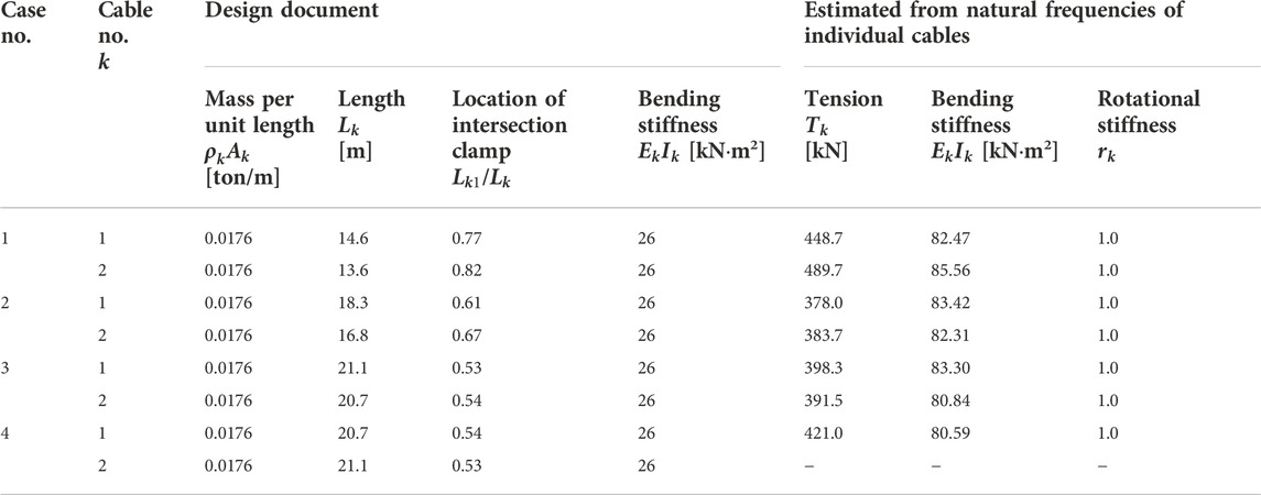
TABLE 4. Specifications of cables considered in field experiment.

The tension, bending stiffness, and rotational stiffness of an individual cable were estimated by considering the first to seventh natural frequencies of the individual cable using the formula proposed by Utsuno et al. (1998). The natural frequencies of the individual cable were measured after removing the intersection clamp. The estimated values are listed in the three right columns of Table 4. The tension estimation error of the method proposed by Utsuno et al. (1998) has been reported to be within 5%. Owing to time constraints, the vibration experiment of cable 2 in case 4 was not carried out, and the tension, bending stiffness, and rotational stiffness of this cable were not estimated.

Regarding the bending stiffness, the estimated value is approximately three times the value in the design document. The bending stiffness in the design document was calculated by the empirical design formula $E_k{I}_k=\frac{1}{3}{E}_k\frac{\pi D_k^4}{64}$, where $D_k$ is the cable diameter. Because the cable is a bundle of 19 strand steel wires, the second moment of area of the circle with the same diameter is divided by three in the design document. The estimation result indicates that the estimated bending stiffness is closer to that obtained by $E_k{I}_k=E_k\frac{\pi D_k^4}{64}$ for a uniform circular cross-section. However, because the bending stiffness has low sensitivity to lower-mode natural frequencies (Yamagiwa et al., 2000), the bending stiffness estimation accuracy is not as high as the tension estimation accuracy.

Regarding the rotational stiffness, the estimated value was 1.0. Therefore, the support condition seems to be closer to fixed support rather than simple support.

4.3 Measured natural frequencies of two cables connected by intersection clamp

In the vibration experiment considering two cables connected by an intersection clamp, cable 1 was hit with a hammer in the out-of-plane direction. The free vibration in the out-of-plane direction was measured by four accelerometers. Then, the measured acceleration histories were transformed into acceleration Fourier spectra, and the dominant frequencies were read as the natural frequencies. The vibration experiment was conducted three times for cases 1 and 4, and twice for cases 2 and 3. In each experiment, the accelerations were measured by four sensors. Therefore, cases 1 and 4 have 12 acceleration data, and cases 2 and 3 have 8 acceleration data. The natural frequencies of the 12 or 8 acceleration data were averaged and used in the estimation.

The acceleration Fourier spectra of one experiment for each case are shown in Figure 9. The average natural frequencies are listed in Table 5. The natural frequencies are round off to three decimal places after taking the average. The first to ninth natural frequencies were used in the estimation.

FIGURE 9

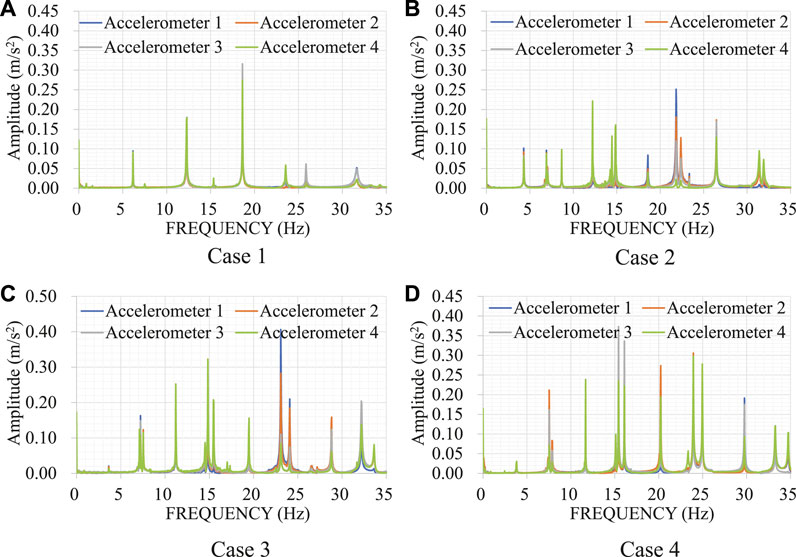
FIGURE 9. Acceleration Fourier spectra measured in field experiment. (A) Case 1. (B) Case 2. (C) Case 3. (D) Case 4.

TABLE 5

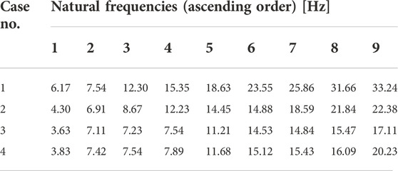
TABLE 5. Measured natural frequencies of two cables with intersection clamp in field experiment.

4.4 Analysis conditions in solution of optimization problem

In the solution of the optimization problem expressed by Eq. 39, the number of sets of initial values in the MultiStart method was 200. It was confirmed that the estimation result was approximately the same even when the number of sets of initial values exceeded 200.

The search range for tension was set to 0.5–2 times the value estimated from the natural frequencies of a single cable. The search range for the bending stiffness was set to 0.26–5 times the design value. The upper bound of the search range for the bending stiffness was set to five times the design value, because the value estimated from the natural frequencies of the individual cable is approximately three times the design value. The search range for the rotational stiffness was 0–1.

4.5 Estimation results

4.5.1 Tension estimation results

The tension estimation results obtained by the proposed method are presented in Table 6. The estimation accuracy is discussed under the assumption that the tension estimated from the natural frequencies of the individual cable (reference value) is true. The reference value of cable 2 ($T_2$) in case 4 was not estimated and the value of cable 1 ($T_1$) was used instead, assuming that the tension of the two cables in case 4 is the same because the tension of the two cables is similar in cases 2 and 3. The estimation errors of all cables are within 10%, which was the target of this study.

TABLE 6

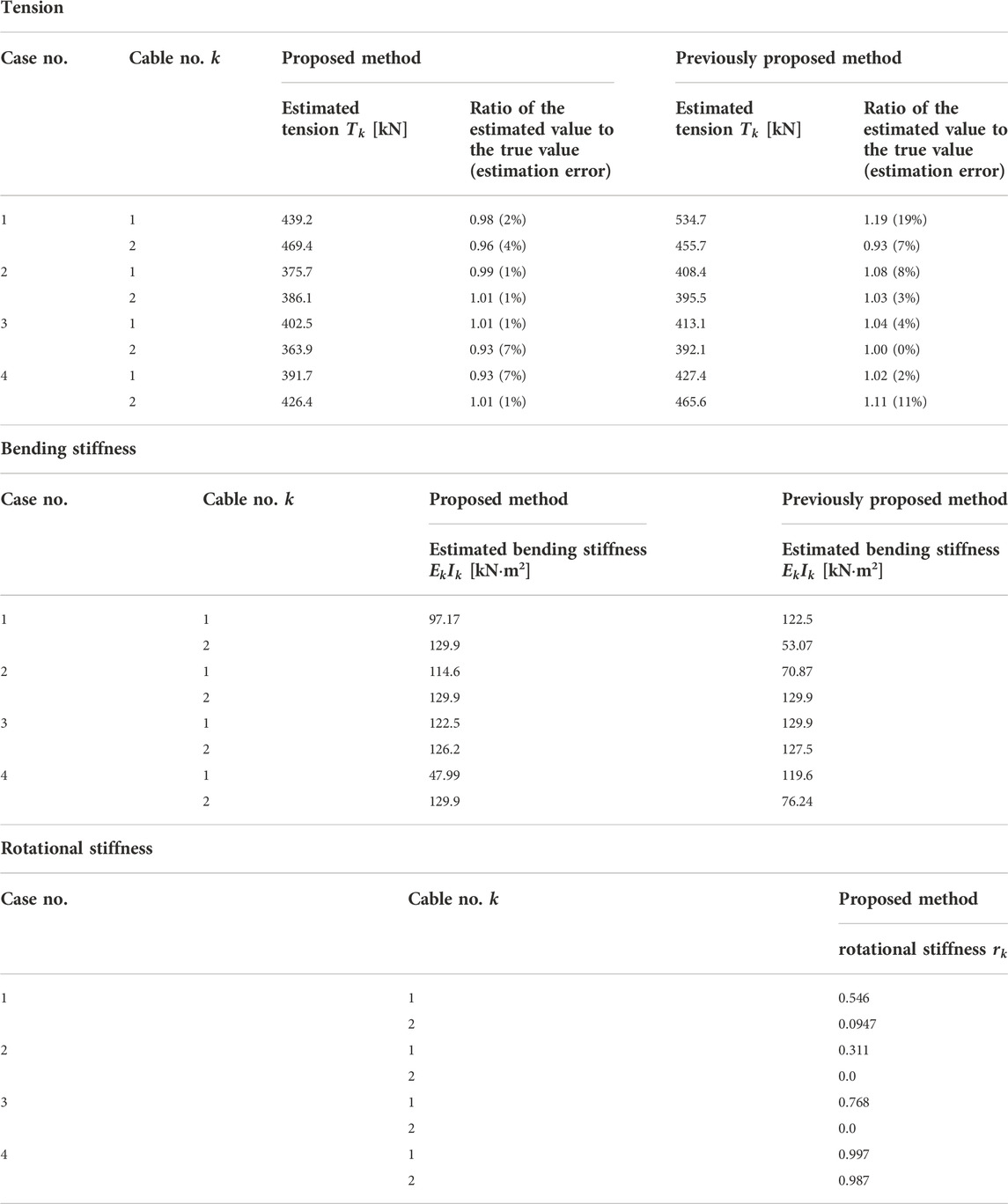
TABLE 6. Estimation results obtained by field experiment.

For comparison, the estimation results obtained by the previously proposed method (Furukawa et al., 2022c) are presented in Table 6. Because the previous method assumes that both ends are simply supported, it tends to overestimate the tension. The tension estimated by the previously proposed method is larger than that estimated by the newly proposed method, except cable 2 in case 1. The estimation error of cable 1 in case 1 is the largest, and its tension is overestimated by 20%. This indicates the necessity of properly treating the rotational stiffness. For cable 2 in case 3 and cable 1 in case 4, the tension estimated by the previous method is closer to the reference (true) value compared with that estimated by the proposed method. However, this does not mean that the previous method is superior. The proposed method underestimated the tension of cable 2 in case 3 and cable 1 in case 4, owing to measurement error, while the previous method tended to overestimate. Therefore, the tension estimated by the previous method is closer to the true value.

In conclusion, the tension of all cables was accurately estimated, and the estimation error is less than 10%. Therefore, the validity of the proposed method is confirmed.

Interestingly, the tension estimation error of cable 2 is less than 10% in cases 2, 3, and 4, wherein accelerometers were only placed onto cable 1 and vibration was excited by hitting cable 1 with a hammer. Accelerometers were not placed onto cable 2. When two cables are connected and vibrate in unison, the required natural frequencies can be recorded by installing accelerometers onto one cable. Moreover, in cases 2 and 3, four accelerometers were placed near the girder at a certain height reachable by ladder. This indicates that it is sufficient for accelerometers to be installed on only one cable at a certain height reachable from the girder by ladder, which greatly improves the inspection efficiency.

4.5.2 Bending stiffness estimation results

The bending stiffness estimation results obtained by the newly proposed and previously proposed methods are presented in Table 6. The values estimated by the two methods are different. Moreover, the estimated values in Table 6 are also different to the design values and values estimated from the natural frequencies of single cables, as presented in Table 4. The reason for this is that the bending stiffness is not sensitive to lower-mode natural frequencies, and the lowest nine modes are considered in the estimation. This tendency of low estimation accuracy for the bending stiffness is similar to the numerical verification results.

4.5.3 Rotational stiffness estimation results

The rotational stiffness estimation results obtained by the proposed method are presented in Table 6. Only the result of the rotational stiffness in case 4 was 1, which is in good agreement with the estimation result obtained for a single cable. The rotational stiffness of cable 2 in cases 1, 2, and 3 is substantially underestimated. The estimation accuracy is low, and this tendency is similar to the numerical verification results.

5 Conclusion

This paper proposes a new method for estimating the tension of two cables connected by an intersection clamp without requiring the removal of the intersection clamp. The proposed method can estimate the tension of two cables in a Nielsen–Lohse bridge from the natural frequencies of the cables. There are many Nielsen–Lohse bridges with short cables, and for short cables, the boundary conditions at both ends of the cable greatly affect the natural frequencies. Therefore, it is necessary to properly model the boundary conditions at both ends of the cable. With this background, the proposed method considers the cable as a tensioned Euler–Bernoulli beam supported by rotational springs at both ends. This study derived a formula for estimating the tension, bending stiffness, and rotational stiffness of two cables simultaneously from the natural frequencies in the out-of-plane direction. In the case of fixed support, the rotational spring constant becomes infinity. It was found that the infinite rotational spring constant in the proposed estimation formula deteriorates the estimation accuracy. To overcome this difficulty, normalization was introduced into the proposed method to avoid infinity in the calculation.

The validity of the proposed method was verified through numerical simulations and field experiments on an actual Nielsen–Lohse bridge. The following conclusions were drawn from this study.

In the numerical verifications, the natural frequencies of the first to ninth mode were used in the estimation, because it is known that tension is sensitive to lower-mode natural frequencies.

First, the effect of the boundary conditions on the tension estimation accuracy was investigated for models with different rotational stiffness and cable length.

The method ignoring the rotational stiffness overestimated the cable tension, particularly for short cables whose cable ends have rotational stiffness. In the case of a 10-m cable with fixed support, the tension was overestimated by approximately 10%. In contrast, the proposed method accurately estimated the tension regardless of the rotational stiffness and cable length.

Next, the validity of the proposed method was verified for 42 models. The proposed method accurately estimated the tension with an estimation error of less than 5% for all 42 models. In contrast, the bending stiffness and rotational stiffness estimation accuracy is low owing to these properties’ low sensitivity against the objective function of the lower modes.

The effect of the natural frequencies’ measurement error on the tension estimation accuracy was also investigated. The tension estimation error was evaluated using two indices, namely, RMSER and MAER. It was found that the RMSER and MAER remained within 0.1 (10%) when the error rate was less than 0.024 and 0.02. When the average of 10 sets of nine natural frequencies was used for estimation, RMSER and MAER were below 0.1 (10%) when the error rate was below 0.092 and 0.056. Taking the average of the natural frequencies obtained from multiple measurements is an effective way for reducing the effect of measurement error.

Finally, the proposed method was verified by a field experiment on an actual Nielsen–Lohse bridge. Four sets of two cables, that is, cases 1–4, were tested. The lowest nine measured natural frequencies were used in the estimation. The tension of eight cables (two cables with four cases each) was accurately estimated, and the estimation error was less than 10%, which confirms the validity of the proposed method.

In cases 2, 3, and 4, accelerometers were only installed onto cable 1, and the vibration was excited by hitting cable 1 with a hammer. Accelerometers were not installed onto cable 2. However, the tension of cable 2 was estimated with good accuracy. In cases 2 and 3, four accelerometers were placed near the girder. This indicates that it suffices for accelerometers to be installed on only one cable near the girder, which greatly improves the inspection efficiency.

As previously mentioned, the current practice of estimating the tension of Nielsen–Lohse bridges requires the removal of intersection clamps. The natural frequencies of each cable are separately measured, the single-cable tension estimation method is applied to each cable, and the intersection clamps are finally reinstalled. The intersection clamps are often installed high above the girders, and their removal and re-installation are time-consuming and laborious because they require an aerial work platform and traffic control. The proposed method simultaneously estimates the tension of two cables without requiring the removal of intersection clamps. Therefore, the proposed method is very useful and greatly improves the efficiency of tension estimation work because it eliminates the need for an aerial work platform and traffic control.

In future work, a statistical tension estimation method will be developed to handle uncertainties and improve the estimation accuracy.

Data availability statement

The original contributions presented in the study are included in the article/supplementary material, further inquiries can be directed to the corresponding author.

Author contributions

AF developed the proposed method, wrote the source code, carried out the numerical analysis, and wrote the article. KK carried out the numerical analysis and wrote the article. MS conducted the verification experiment.

Acknowledgments

We thank Edanz (https://jp.edanz.com/ac) for editing a draft of this manuscript.

Conflict of interest

Author MS was employed by Kobelco Wire Company, Ltd.

The remaining authors declare that the research was conducted in the absence of any commercial or financial relationships that could be construed as a potential conflict of interest.

Publisher’s note

All claims expressed in this article are solely those of the authors and do not necessarily represent those of their affiliated organizations, or those of the publisher, the editors and the reviewers. Any product that may be evaluated in this article, or claim that may be made by its manufacturer, is not guaranteed or endorsed by the publisher.

References

Chen, C. C., Wu, W. H., Leu, M. R., and Lai, G. (2018). A novel tension estimation approach for elastic cables by elimination of complex boundary condition effects employing mode shape functions. Eng. Struct. 166, 152–166. doi:10.1016/j.engstruct.2018.03.070

CrossRef Full Text | Google Scholar

Chen, C. C., Wu, W. H., Leu, M. R., and Lai, G. (2016). Tension determination of stay cable or external tendon with complicated constraints using multiple vibration measurements. Measurement 86, 182–195. doi:10.1016/j.measurement.2016.02.053

CrossRef Full Text | Google Scholar

Fang, Z., and Wang, J. Q. (2012). Practical formula for cable tension estimation by vibration method. J. Bridge Eng. 17 (1), 161–164. doi:10.1061/(asce)be.1943-5592.0000200

CrossRef Full Text | Google Scholar

Furukawa, A., Hirose, K., and Kobayashi, R. (2023). “Tension estimation method for cable with damper and its application to real cable-stayed bridge,” in Experimental Vibration Analysis for Civil Engineering Structures. Editors Wu, Z., Nagayama, T., Dang, J., and Astroza, R. (Cham: Springer), Vol. 224. doi:10.1007/978-3-030-93236-7_32

CrossRef Full Text | Google Scholar

Furukawa, A., Hirose, K., and Kobayashi, R. (2021). Tension estimation method for cable with damper using natural frequencies. Front. Built Environ. 7, 603857. doi:10.3389/fbuil.2021.603857

CrossRef Full Text | Google Scholar

Furukawa, A., Suzuki, S., and Kobayashi, R. (2022a). Tension estimation method for cable with damper using natural frequencies with uncertain modal order. Front. Built Environ. 8, 812999. doi:10.3389/fbuil.2022.812999

CrossRef Full Text | Google Scholar

Furukawa, A., Suzuki, S., and Kobayashi, R. (2022b). Tension estimation method for cable with damper using natural frequencies and two-point mode shapes with uncertain modal order. Front. Built Environ. 8, 906871. doi:10.3389/fbuil.2022.906871

CrossRef Full Text | Google Scholar

Furukawa, A., Yamada, S., and Kobayashi, R. (2022c). Tension estimation methods for two cables connected by an intersection clamp using natural frequencies. J. Civ. Struct. Health Monit. 12, 339–360. doi:10.1007/s13349-022-00548-6

CrossRef Full Text | Google Scholar

Furukawa, A., Yamada, S., and Kobayashi, R. (2022d). Tension estimation methods for Nielsen-Lohse bridges using out-of-plane and in-plane natural frequencies. Int. J. GEOMATE 12 (2). 603857. doi:10.21660/2022.97.3235

CrossRef Full Text | Google Scholar

Harada, M., Kajikawa, Y., and Fukada, S. (2002). Survey of the nielsen-lohse bridge after 30 years. Proc. 57th Annu. Meet. Jpn. Soc. Civ. Eng. 57 (I-290), 579–580.

Google Scholar

Kuriyama, T., Bing, Y., and Horiuchi, H. (1994). A proposal for a tension measurement method for cable with clamps on nielsen bridge. 49th Annu. Lect. Civ. Eng. Soc. (CSC) I-176, 350–351.

Google Scholar

Ma, L. (2017). A highly precise frequency-based method for estimating the tension of an inclined cable with unknown boundary conditions. J. Sound Vib. 409, 65–80. doi:10.1016/j.jsv.2017.07.043

CrossRef Full Text | Google Scholar

MathWorks (2020). MATLAB documentation, MultiStart. AvaliableAt: https://jp.mathworks.com/help/gads/multistart.html (Accessed June 13, 2022).

Google Scholar

Nam, H., and Nghia, N. T. (2011). Estimation of cable tension using measured natural frequencies. Procedia Eng. 14, 1510–1517. doi:10.1016/j.proeng.2011.07.190

CrossRef Full Text | Google Scholar

Sakano, M., Kitada, T., and Chono, K. (2003). Mechanical properties of Nielsen-Lohse bridges and their load-bearing capacity. Proc. Soc. Civ. Eng. Struct. Eng. 49A, 93–104.

Google Scholar

Sakoda, H., Zui, H., Kagayama, T., Uehira, S., Kitada, T., and Nakai, H. (2000). On causes of loosening and slackness of hanger cables in a Nielsen-Lohse bridge due to Hyogo-ken Nambu earthquake. Proc. Steel Constr. 7 (25), 31–42. doi:10.11273/jssc1994.7.31

CrossRef Full Text | Google Scholar

Shinke, T., Hironaka, K., Zui, H., and Nishimura, H. (1980). Practical formulas for estimation of cable tension by vibration method. Proc. Jpn. Soc. Civ. Eng. 294, 25–32. doi:10.2208/jscej1969.1980.294_25

CrossRef Full Text | Google Scholar

Shinko Wire Company (2017). Tension measuring technique for outer cables. AvaliableAt: http://www.shinko-wire.co.jp/products/vibration.html (Accessed June 13, 2022).

Google Scholar

Utsuno, H., Yamagiwa, I., Endo, K., and Sugii, K. (1998). Vibration transfer function method to estimate tension and flexural rigidity of cable. J. Struct. Eng. A 44 (2), 853–860.

Google Scholar

Wu, W. H., Chen, C. C., Chen, Y. C., Lai, G., and Huang, C. M. (2018). Tension determination for suspenders of arch bridge based on multiple vibration measurements concentrated at one end. Measurement 123, 254–269. doi:10.1016/j.measurement.2018.03.077

CrossRef Full Text | Google Scholar

Yamagiwa, I., Utsuno, H., Endo, K., and Sugii, K. (2000). Identification of flexural rigidity and tension of the one-dimensional structure by measuring eigenvalues in higher order. Trans. JSME(C). 66 (649), 2905–2911. doi:10.1299/kikaic.66.2905

CrossRef Full Text | Google Scholar

Yan, B., Chen, W., Yu, J., and Jiang, X. (2019). Mode shape-aided tension force estimation of cable with arbitrary boundary conditions. J. Sound Vib. 440, 315–331. doi:10.1016/j.jsv.2018.10.018

CrossRef Full Text | Google Scholar

Yoneda, M. (2000). Effect of lifting materials on the structural damping of Nielsen-type Lohse-girder bridges. Dob. Gakkai Ronbunshu 651 (IV-47), 157–162. doi:10.2208/jscej.2000.651_157

CrossRef Full Text | Google Scholar

Zui, H., Shinke, T., and Namita, Y. (1996). Practical formulas for estimation of cable tension by vibration method. J. Struct. Eng. (N. Y. N. Y). 122 (6), 651–656. doi:10.1061/(asce)0733-9445(1996)122:6(651)

CrossRef Full Text | Google Scholar