 Malek Ghanem1
 Farook Hamzeh
 Olli Seppänen
 Lynn Shehab
- 1Civil and Environmental Engineering Department, American University of Beirut, Beirut, Lebanon
- 2Civil and Environmental Engineering Department, University of Alberta, Edmonton, AB, Canada
- 3Civil Engineering Department, Aalto University School of Engineering, Espoo, Finland
Push planning and pull planning are different approaches used for production planning and control. Push planning uses predetermined dates to control a project, whereas pull planning utilizes the system’s current state. Although researchers have compared these approaches from production planning perspective to improve project performance, the differences between push and pull in construction and their impacts on crew performance and congestion have not yet been explored. Therefore, this research aims to investigate the underlying mechanisms of applying pull and push approaches at the location level through simulation, in addition to proposing hypotheses relating push and pull approaches to project and crew performance metrics. Agent-based modeling is used to simulate and describe how push and pull approaches affect crew performance. Results show that pull approaches can achieve significantly higher productivity, less idle time, lower crew turnover, and fewer task interruptions, although they can result in slightly increased project durations. Cross-analyzing the mentioned results with other performance metrics reveals that push and pull approaches should be applied together to achieve a flexible production control system. The significance of this study is embedded in exploring and understanding how the choice of push and pull planning approaches impacts the location-based management of tasks and crew performance. Such impacts on productivity, crew performance, and the flow of site operations enable a convergence to generalized conclusions regarding the efficacy of each method.
Introduction
The construction industry is known for a trifecta of issues: complexity, uniqueness, and uncertainty (Trinh and Feng 2020) where the level of complexity is related to how complicated management issues are (Bennett 1991). This implies several challenges that need to be considered during the planning, scheduling, and monitoring phases of the execution process. Fragmentation, unpredictable events, and variability are all factors that require constant updates of construction schedules (Dallasega et al., 2021). Fragmentation leads to local optimization by each crew who are not necessarily motivated to follow the General Contractor’s schedule (Sacks and Harel 2006). Furthermore, poor jobsite management can lead to workspace interference if workspace dynamism is not managed accurately. Workspace interference includes unexpected space overlaps among crew and resources, which lead to losses in productivity and project delays (Sanders and Thomas 1991; Dawood and Mallasi 2006; Hosny et al., 2020).
Interference and space congestion are correlated to the production planning and control methods used on a project. Hopp and Spearman (2004) identified two types of control systems: pull and push. While push systems plan work in the system based on a predetermined plan, pull systems operate by redirecting resources based on the state of the production system. These concepts originated from manufacturing, with various attempts to apply them in construction. Researchers have often considered the traditional and widely used critical path method (CPM) a push system, due to its focus on pushing activities on the critical path (Tommelein 1998). In contrast, location-based methods, such as location-based management system (LBMS) (Kenley and Seppänen 2010) and methods based on systematic evaluation of constraints, such as the Last Planner System (Ballard 2000), have often been described as pull systems. Hopp and Spearman (2004) stated that the term pull production has become a cornerstone of modern manufacturing, which requires limiting the amount of work-in-process and executing tasks based on the readiness of the work and the subsequent trades (Hopp and Spearman 2004). Gayer et al. (2021) assessed pull production systems in three industries: manufacturing, healthcare and construction. Their results related to construction showed pull principles implemented using the Last Planner System, Kanban cards and visual management. However, their study focused on single trade, masonry, and did not consider the impact of pull when facing variability. Although theoretical comparisons between the two production systems have been made (e.g., Olivieri et al., 2018), they are mostly based on comparing flow of resources between locations in planned schedules.
Previous research has neither studied the impact of push and pull in the construction phase in terms of control actions employed when facing project delays nor investigated their impacts on crew productivity. Decision making on crew level has been neglected. In reality, production crews have significant autonomy and continuously make decisions when the original plan cannot be exactly implemented because of variability (Lehtovaara et al., 2022). The presented gaps are of high importance, since crew behavior and the on-site level of interaction between them can change the overall project performance by affecting productivity, project duration, labor cost, and other essential metrics (Watkins et al., 2009).
To address the mentioned research gaps, this paper aims to provide a deeper understanding of the underlying mechanisms of applying pull and push approaches at the location level and of their usage, or lack thereof, in the industry. It investigates production planning and control systems, evaluates push and pull control approaches at the level of crew decision-making through simulation, and addresses the effect of these approaches on labor productivity, crew logistics, allocation to areas, crew movement, and crews’ interactions within a project. These objectives are addressed using agent-based modeling (ABM) for push and pull scenarios and by measuring several performance metrics that help in contrasting these techniques, investigating optimal approaches, and gaining insights into process behavior. Data from an actual construction project was used to test the proposed model.
Literature review
Construction management comprises planning, coordinating, executing, and controlling operations to achieve the set targets (Knotten et al., 2015). Construction operations rely heavily on the availability of resources such as workforce, equipment, materials, and finances (Halpin et al., 2017). This research addresses both pull and push production planning and control systems as well as operational decision making at the crew level.
Production planning and control
The approach selected for managing construction production flow, which is concerned with the adequate allocation of resources to production activities, plays a pivotal role in directing the project towards successful delivery (Hamzeh et al., 2019). Since some traditional production planning and control practices are reactive in nature, researchers have likened them to a “thermostat” model of production control (Mantel and Meredith 2003), which increases waste and variability. Traditional planning and control approaches tend to mainly apply push-driven techniques. Project control then tries to maintain the planned schedule during execution, assuming that all the resources needed to start an activity will be available once an activity start date is reached (De Toni et al., 1988). Thus, activities are released when their predecessors have been completed. This view ignores the constraints that are typically not modeled in the network but are required to start the activity, such as availability of material, information, labor, equipment, space, and good working conditions, as well as previous work being completed (Koskela 2004). When some perquisites are available and others are lacking, the activity start either waits for the missing resources, or the activity may start with partial requirements, creating what is called making-do waste (Koskela 2004), which can negatively impact productivity (Thomas et al., 1989; Howell et al., 1993; Tommelein 1998). The critical path method (CPM) has been criticized for shortcomings associated with ensuring requirements, generating a poor workflow and crew continuity problems (Arditi et al., 2002; Hamzeh et al., 2015).
In contrast, location-based methods, such as LBMS were developed to explicitly model crew movements in a construction project. This system aims to increase workflow reliability while reducing variability and its negative impacts (Kenley and Seppänen 2010). The LBMS bases all planning and control on a fixed location breakdown structure (LBS) where tasks are undertaken by crews flowing through location (Kenley and Seppänen 2010). To visualize crew workflow, LBMS uses flowline visualization, showing task completion in each location versus time. These lines may have a gentle or a steep slope depending on their corresponding production rates. This allows the visualization of “bottleneck” tasks, which have flat slopes, and allows for optimization through adjusting the slope by changing the number of crews, or scope, or through changing the location sequence, splitting tasks, or other approaches (Kenley and Seppänen 2010). During execution, schedule forecasts are used to guide production. The actual production rate of a task is used to calculate forecasts and assumes the production rate continues at the same rate unless control actions are taken. Production control focuses on upcoming alarms when two tasks are about to interfere (Seppänen et al., 2014). This approach explicitly considers the current state of space and resource constraints and, from that point of view, can better enable a pull control approach (Seppänen 2009).
The theoretical pull approach is not enough to address all productivity issues because of the high variability of construction processes. Both CPM and LBMS schedules can account for uncertainties that could arise during execution, such as uncertainty in duration and dependency logic. However, managing these uncertainties during task execution requires adhering to the planned schedule, because actual network conditions and resource availability may differ from those assumed during planning (Tommelein 1998). Thus, although CPM as a planning system is often associated with push and LBMS is often associated with pull, it is more critical to evaluate how production is controlled when deviations from the schedule occur. Although previous authors have extensively documented differences between CPM and LBMS approaches in the theoretical planning phase (Arditi et al., 2002; Seppänen 2009; Kenley and Seppänen 2010; Olivieri et al., 2018), the previously documented differences are not related to push or pull. Both the CPM and the LBMS result in start and finish dates that can be used to push production, if the current status of the constraints is not considered, or pull production, if the current status of the constraints is considered. The analysis of these approaches based on push and pull during execution phase has not been performed in previous research.
Pull and push techniques at the crew level
Generally, pull exhibits downstream work processes pulling materials from an upstream work process, enabling reducing the amount of work in process compared to push techniques (Kalsaas et al., 2015). From a crew-level standpoint, crew-level decision making is associated with the assignments a crew should perform next (Hosny et al., 2020) or whether additional crews need to be mobilized and others demobilized. Based on the definition of push and pull systems by Hopp and Spearman (2004), these decisions are made based on a predetermined plan in push systems or based on the status of the system in pull systems.
Since resource management is one crucial factor in developing reliable schedules (Damci et al., 2013), traditional construction planning employs a push approach where all resources required to perform an activity are assumed to be available at the planned start date of that activity (Tommelein 1998). Some disadvantages of the push approach include the fact that work-in-progress can build up in front of a workstation with unexpected downtime (Kalsaas et al., 2015). In construction, this could be translated to idle activities due to unavailable prerequisites or unresolved constraints of a given activity, leading to a bottleneck in construction workflow. On the other hand, the pull approach ensures selective drawing of resources to be accessed by activities whose output is needed further downstream in the process (Tommelein 1998). This approach also aims to improve productivity by reducing inventories that can negatively impact the smooth workflow of a project (Ghosh et al., 2017).
Therefore, in construction, a pure push approach focuses on reducing variances from a predetermined schedule without considering the status of the system. As shown in Figure 1A, when the crew finishes one activity (A) in a location and needs to perform the same activity in another location (B, B′, or B″), in a push approach the crew moves to the task/location pre-set by the schedule without considering the current status of material availability, material hauling distance, congestion caused by other crews in that location, proximity between locations, and other constraints (Ghanem et al., 2018). In this specific example, the schedule depicts that crews should move to task B″ in a location that 1) is more congested relative to other available areas, 2) requires hauling material over a greater distance compared to other areas, and 3) is farther relative to available locations. Considering a pull approach for the same scenario, Figure 1B shows how all three alternative locations are assessed, and the schedule, material availability, and anticipated production rate or congestion in the available locations are considered. The main purpose of evaluating these alternatives is to choose the location that allows for greater labor productivity based on the state of the system (actual conditions of congestion, material availability, etc.). Therefore, push and pull processes operate differently when crews decide which assignments to do next.
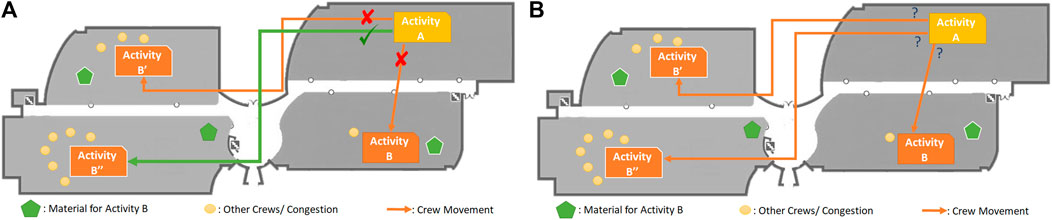
FIGURE 1. Crew logistics for moving between activities following (A) a push system and (B) a pull system.
Push and pull approaches lead to differences in overall resource allocation when determining when to increase the number of crews on site. Since push control is based on trying to achieve the planned schedule, subcontractors tend to allocate more crews to a late activity in order to increase its production rate (Seppänen 2012; Frandson et al., 2015). Push approaches thus increase crew sizes when tasks are delayed, which may cause overstaffing and result in productivity losses (Thomas 1992). In contrast, pull approaches consider the ability of locations to accommodate crews and thus are expected to reduce the negative impacts on productivity. In effect, empty locations pull crews (Seppänen 2009), where assignments are released to production units only when all the prerequisites of production are available (Ballard 2000). In pull approaches, additional crews are mobilized when production falls behind the production rate of the predecessor task (Seppänen 2009).
Therefore, when evaluating the impact of push and pull control on project success, the literature highlights several key differences, as shown in Table 1. Differences related to production planning have already been evaluated (Olivieri et al., 2018). There is less understanding on the impact of deciding assignments on crew level and decisions on resource mobilization. The aim of this research is to explore quantitatively the differences between pull and push, focusing on the execution phase. Agent-based modeling is used to address these issues by modelling push and pull production planning scenarios and measuring several performance metrics that help in contrasting these techniques and reaching optimal approaches and recommendations.
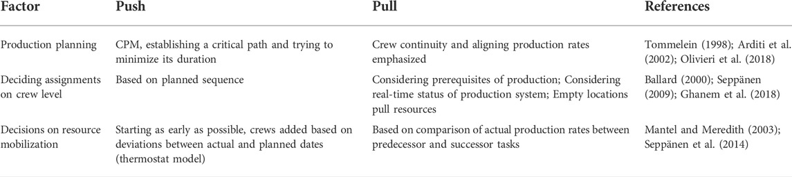
TABLE 1. Key differences between push and pull in construction projects.
Research methods
Because the objective was to investigate crew behavior under dynamic conditions, we selected Agent-Based Modeling (ABM) as the most suitable approach. ABM is a technique that has been used relatively recently to model complex systems of interacting agents (Raoufi and Fayek 2015). Agents are considered the main constituents of ABM and can be described as software entities capable of studying their own local environments and autonomously executing their assigned tasks. They interact as they communicate with each other and modify their behaviors to achieve their goals (Chen et al., 2013). A collection of static and dynamic attributes is assigned to agents, leading them to behave uniquely (Macal and North 2011).
Different research studies have adopted ABM for various objectives. For example, Barakat and Khoury (2016) used ABM to study occupant multi-comfort level to reduce energy consumption within academic buildings. Haryadi et al. (2019) predicted future rooftop photovoltaic adoption through ABM to understand the impact of the decision-making behavior on electricity utilization. Feng et al. (2019) proposed an ABM approach to model and evaluate the reliability and performance of a complex human–machine system through a case study of an aircraft carrier. ABM has also been employed for educational studies where a model was developed to assist teachers in simulating their teaching strategies to ultimately quantify their influence on group sociometrics such as dissociation, coherence of reciprocal relations, cohesion, and density of relations (Garcia-Magarino et al., 2020). In a different context, ABM was used to investigate potential plug-in hybrid electric vehicles (PHEV) consumer adoption to identify interactions among potential leverage points that may affect PHEV market penetration (Eppstein et al., 2015).
ABM was chosen for this research, because of the two main topics of comparison: the decision making on crew level and when to mobilize new crews. Different decisions made by crews cause dynamic conditions when crews interact with each other. These complex interactions are hard to express through regular analytic mathematics. ABM allows each crew to have a utility function that they use to decide where to work next. The push approach weighs the top-down plan more than the pull approach, which prioritizes locations based on the prerequisites (i.e., available locations pull crews).
To create a realistic test case for simulation, data from real construction project were used. The project was a 25,000 m2, three story medical office building mainly housing physicians’ offices and examination and procedure rooms and located in California, United States. Data included the necessary information to build the model, such as crews along with their attributes, activities and tasks, the site layout, and the exact areas of locations. This project was selected due to the availability of data and the appropriate level of project complexity needed to demonstrate and contrast pull and push planning.
A framework was adopted for testing the effects of push and pull approaches on location-level crew productivity and project performance as shown in Figure 2. The following steps were followed for this study: 1) a literature review was conducted of different production planning and control techniques discussed in addition to a brief analysis of how push and pull approaches affect productivity; 2) problem identification and research objectives identify and address research gaps in the literature; 3) conceptual and computational models were developed that represent the agent-based model’s mechanisms, inputs, parameters, variables, and outputs; 4) model validation and verification was conducted to check whether “we built the right model” and “we built the model right,” respectively; 5) model experiments generated multiple simulation runs of push and pull scenarios; and 6) results were analyzed and comprehensive conclusions and recommendations were proposed.
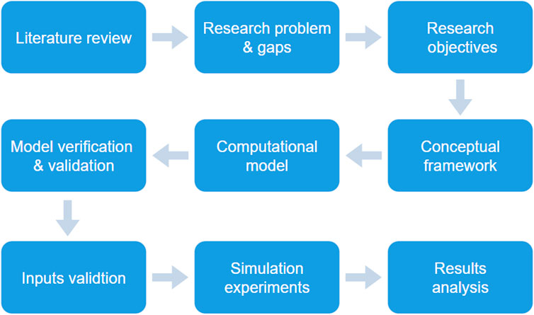
FIGURE 2. Methodology steps.
Conceptual framework
Prior to building the simulation model, a conceptual framework was developed to evaluate the effects of push versus pull approaches in production control on different project performance metrics. To test how different approaches affect crew and project-level performance, a model demonstrating how crews work on a construction site, how they interact with each other, and how their productivity is affected was needed. Thus, the model was mainly composed of crews of various trades working in an environment representing a construction site. The activities they perform were also modeled, each having various parameters including space required by crews, locations, predecessor tasks, successor tasks, and resources needed for each activity. The activities considered included drywalling, casework, several mechanical, electrical, and plumbing (MEP) works, painting, and other finishing activities. The model simulated push scenarios where activities are selected based on a pre-set schedule and pull scenarios where activities are executed based on the status of the system. The model specifically considered physical constraint types, such as space, resources, and material logistics, and ignored others, such as design or work conditions. However, the focus of this study is decision-making on crew level and mobilization of additional crews, whereas material logistics techniques will be integrated in future research.
Agent-based simulation model
After developing a conceptual framework, the working environment and the dynamic interactions between crews and activities were modeled using ABM through the simulation software “AnyLogic 7.3.1.” The main environment considered in this study is the construction site, where crews of different trades interact and work together on different activities. The main agent types used were Crew, Activity, and Location. Figure 3 shows the environment and the agents along with their attributes. As shown in Figure 3, every agent has the attributes required to track its behavior and its relationship to other agents. To initialize the model in a logical manner, data used to initialize the agent’s attributes and parameters were obtained from a real construction project, which was a medical office building located in California, United States. This is discussed further in the validation section.
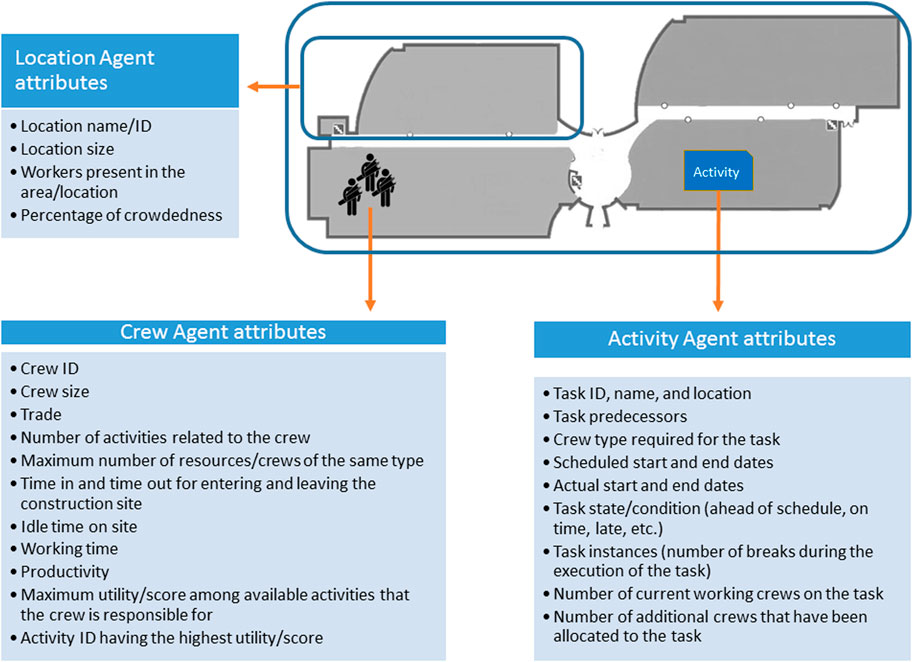
FIGURE 3. Main environment and the agents along with their attributes.
Crew agents
Crew agents represent all crews of different trades. The behavior and level of interaction between Crew agents on-site can change the project’s performance metrics. These crews are represented in AnyLogic by a population of “Crew” agents, each having the attributes shown in Figure 4.
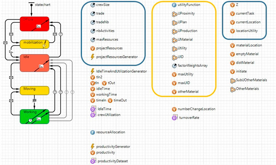
FIGURE 4. “Crew” agent type.
The parameters and variables indicated in the blue zones in Figure 4 are attributes that characterize each crew. Their values vary from one crew agent to the other based on the crew agent’s assigned trade. These parameters contain fixed values that are defined for each crew during model initialization, such as crew size, the number of activities to be executed by each type of crew, and the maximum allowable resources (crews) that can be mobilized to the site if needed. Variables indicated by the blue zones summarize information for each crew that changes during simulation, including the current task a crew is executing and the current location. The orange zone indicates the “Utility function” along with its collections and variables. This function is explained in detail in the following sub-section. Some other events and variables are used to calculate idle time and work time for each crew, which are calculated at the end of each workday as total hours a crew spends in an Idle state or Working state on a given day. Also, the number of locations visited by each crew is recorded.
The state chart shown in Figure 4 indicates behavioral states for each crew along with the conditions that determine the transitions between these states, as described in Table 2.
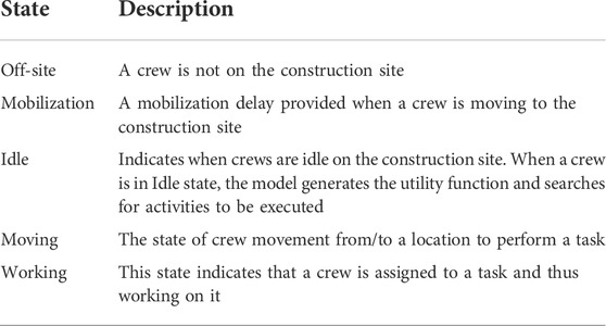
TABLE 2. Behavioral states for each crew agent.
Utility function
Utility functions are required to model decision-making at the crew level. The utility function is the main driver that determines the next task to be performed by each crew and where it is located. This function accounts for push and pull approaches, and it takes into consideration the proximity between locations, the schedule, and anticipated crew production rates. Each of these three factors is translated into a numerical value, which is scored out of 100 and given a certain weight. Then, Eq. 1 is used to calculate a global score, and the task with the highest score is identified as the next task to be executed.
where:
• UProximity accounts for the distance between a crew’s current location and the next location. The assumption is that crews prefer to move to new locations close to their current locations.
• UPlan accounts for the plan/schedule logic. It gives higher scores to activities that should start according to the schedule and lower scores to activities that follow.
• UProduction is the anticipated production rate. It accounts for congestion in places that a crew will move to. Places with relatively less crowding score higher than more congested locations.
• WProximity, WPlan, and WProduction are weights assigned to each factor. These weights change between push and pull scenarios.
In push scenarios, WProximity and WProduction each have a value of 0.1, whereas WPlan has a value of 0.8, indicating that the dominant factor is UPlan. This reflects the fact that production is mainly controlled by the schedule, and the other two factors are given less attention. The weights are chosen based on the synthesis of literature review (Table 1), which highlights the dominance of the project schedule over other factors such as proximity and productivity, which are not considered in the planning and control process of a construction project with a push-driven approach. In a pure push scenario, the decisions in planning and control are entirely based on the thermostat model. However, in this model, a small weight was given to proximity and production rate potential in order to achieve a more realistic scenario where subcontractors still consider their productivity although the general contractor is pushing for implementation of the original plan.
However, in pull scenarios, the three factors are considered as follows: UPlan and UProduction contribute to 70% of the total utility score (both having the same weight of 0.35), whereas UProximity contributes to the remaining 30%, based on Table 1. Pull-driven approaches consider availability, state, and location of resources. Although a pure pull scenario would give no weight to a plan and base the whole decision on proximity and production rate potential, in this study the plan was given the same weight as the production rate in order to achieve a more realistic practical scenario where the plan still has some value. Proximity is also important; however, it is assumed to have less impact on the decision, and even though moving to a closer location within the project is usually better for a crew, the crew spends much less time moving between locations than working in a location, and hence a lower weight was given to UProximity compared to UPlan and UProduction.
Activity agents
This agent population includes all activities and tasks to be executed on the construction site. Each task has a certain location, a fixed quantity of work, and an estimated consumption rate (person-hours/unit) and requires a certain crew. The values of the mentioned attributes vary among the different activities. Activities follow a finish-to-start relationship, meaning an activity has as a predecessor activity. This data is defined in the model.
Note that tasks in the actual construction site CPM schedule did not only have finish-to-start (FS) relationships; they had more complex relationships including finish-to-finish (FF) and start-to-start (SS) with lags. However, for this model, the planned logic for push scenarios was simplified to have only FS relationships, as the aim of the model is to test project control methods rather than project planning techniques.
For pull scenarios, the same logic of an FS relationship is used in addition to ensuring the continuity of activities throughout different locations. It is important to note here that CPM does not allow enforcing continuous work, although it can model resource constraints (Olivieri et al., 2018). In the pull scenario, the schedule was optimized by selecting an optimum number of crews for each activity to ensure aligned production rates. However, both push and pull scenarios used the same resource availability constraints. The parameters of each activity in addition to other attributes are shown in Figure 5.
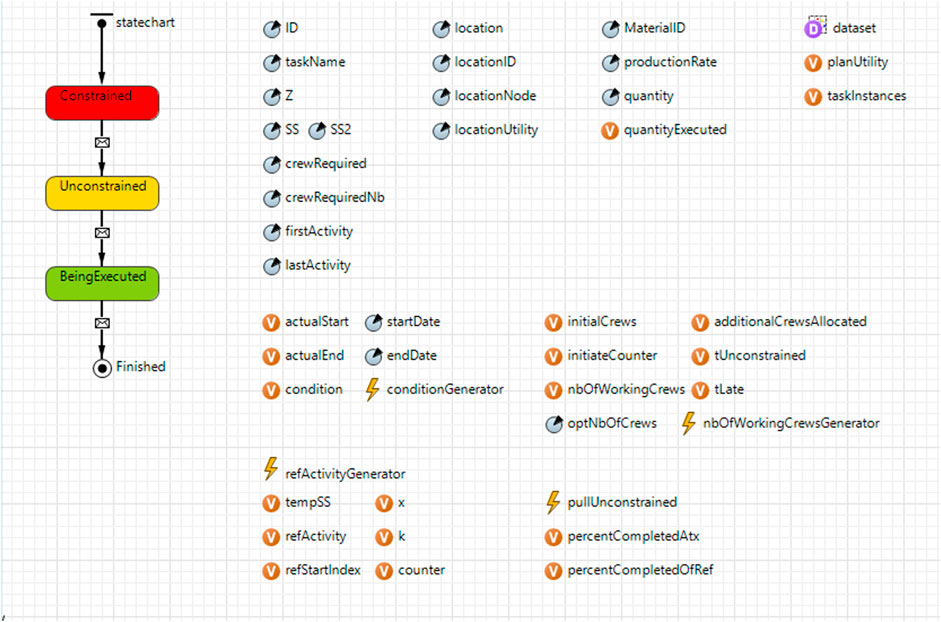
FIGURE 5. “Activity” agent type.
As shown in Figure 5, parameters are used to initialize each task, giving an ID, name, location details, predecessors, crew trade required, expected production rate, and quantity to be executed. Variables are then used to track attributes that change during the simulation time, such as quantity executed, actual start and end dates, the task’s condition, and the number of crews working on the task. Other events such as “Ref. Activity Generator” and “Pull Unconstrained” are explained later in this section.
The methods used in determining a task’s condition—whether it is on time, late, or ahead of schedule—differ between push and pull scenarios. This condition is generated through the “Condition Generator Event.” As discussed in the literature review, push approaches use predetermined plans for decision making. In a push scenario, the condition is determined by comparing the actual percentage completion of the total quantity to the planned percentage of completion for the current date. Therefore, the task is considered late if it is late compared to the predetermined schedule. In contrast, pull approaches use information on the current state of the production system to determine when to act. Therefore, in a pull scenario, the conditions of all activities are based on the current time buffer (the empty time between activities, which can be read horizontally in the flowline diagram) between the reference activity and the activity being considered:
• If the time buffer is increasing, then the task is late (i.e., it is slower than the reference).
• If the time buffer is decreasing, then the task is early (i.e., it is faster than the reference).
• Otherwise, the task is on schedule.
The reference task used in determining the condition of each task, in the case of pull scenarios, is the first continuous task encountered before the activity being studied. A continuous task is a task that has a continuous flowline from one location to another, as indicated in Figure 6. The reference activity is determined by a “Ref. Activity Generator” event. For the first task, the reference task was the planned production rate of the first task. Therefore, the whole production system in a pull scenario attempts to achieve the planned slope for all tasks.
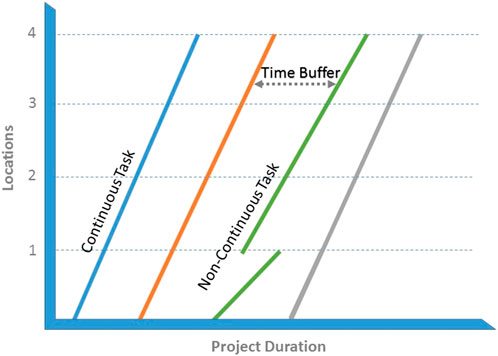
FIGURE 6. Continuous and non-continuous tasks.
Once a task is late, push and pull scenarios handle it differently. More crews are sent to a late task if a push approach is applied, disregarding crew productivity. In the pull approach, crews are assigned to a late task until reaching an optimum number, after which congestion will very negatively affect crews’ productivity. If these crews cannot reach the same production rate for the task as their predecessors, they will be mobilized to any available subsequent location. In this way, empty locations pull resources, and the overall task production rate can be adjusted to match the predecessor if sufficient resources are available. This leads to discontinuity in the flowline diagram for this specific task, but it helps a crew catch up with the previous, faster task. If enough resources cannot be added to a task in currently ongoing locations without a congestion penalty, new locations are opened, making it a non-continuous task.
Model verification and validation
Model verification
To verify the model, extensive testing was performed to assure that “we built the model right.” Several steps were followed such as closely checking coded manuscripts and functions. Temporary parameters and variables were also used to trace different functions and events used in the model and verify that they were used correctly. Moreover, the model’s aim, scope, and scale were evaluated, the data was characterized for testing and calibration, and visual analysis to judge the performance of the model was performed to detect non-modelled behavior (Bennett et al., 2013).
Model validation
Although it is widely agreed that absolute validation is not always possible (Robinson et al., 2004), in order to know whether the “right” model had been built for this study, several validation techniques stipulated by Sargent (2013) were used:
• Animation tests: The model’s operational behavior was validated through the visualization of crews’ movements from one location to another while the model was running. During the simulation, flowlines were displayed and updated every workday, and a reasonable relationship could be drawn between the number of crews working in a location and the slope of the flowline of the corresponding task: more crews working were shown as steeper slopes, representing higher production rates. The level of congestion in locations was also monitored.
• Face validity: Experts knowledgeable about real production planning and control systems were consulted.
• Internal validity: Several simulations with stochastic behavior showed acceptable variability. The results of the metrics that were measured had acceptable standard error values (less than 0.01) within less than 50 runs.
• Operational graphics: Different metrics and variables were dynamically tracked throughout simulation runs. Quantity executed of each task, congestion in each location, idle time, productivity, task conditions, and number of crews working in the same location were updated continuously to keep the data realistic and to use it correctly in functions and events. Each metric and variable was tracked on its own and along with one another to achieve a realistic model behavior. For example, the number of crews working in a location and the level of congestion show a direct relation as they increase and decrease with each other throughout the simulation time.
Validation of inputs
In addition to model validity, data validity is essential, since obtaining sufficient, accurate, and appropriate data is usually difficult, time consuming, and costly (Sargent 2013). In this research, data from an actual construction site were used for model initialization. Data included the necessary information to build the model.
Simulation experiments
After setting up the model, simulation experiments were generated, and different metrics were collected from each run to help in comparing the push and pull production control approaches. These metrics are:
Each metric sheds light on certain aspects that help in assessing the production control approach used. Project total duration (in days) is the time taken to complete all project activities. Total work time (in hours) is the sum of work time of all crewmembers throughout the project. Sum of activities’ start dates is the total of all activity start dates. Sum of activities’ end dates is the total of all activity end dates. Task throughput (no. of tasks) is the number of finished tasks at a given point in time. Total idle time/crew (hrs.) is the total duration a crew is idle. Productivity (units/person-hour) is quantity executed by each crew member during a time interval. Turnover rate (locations visited/time unit) is the frequency with which a crew changes locations per unit of time, including re-entering the same location. Task instances (no. of tasks) is the number of interruptions that occur per task.
Results and discussion
Several hypotheses regarding the effects of push and pull approaches on different project performance metrics were proposed. Then, simulation outputs were collected for each run. A null hypothesis for each metric was first tested by assuming the metrics of both push and pull approaches to be equal. All hypotheses assuming equal metric results were rejected. Afterwards, alternative hypotheses were tested (Table 3). The collected data was tested for normality using a significance level of 5%, and the results showed that the data followed a normal distribution. Test results are aligned with the central limit theorem, which considers that if a sample’s size is relatively large (>30), the data can be assumed to follow a normal distribution. Hence, “Student’s t-test” was conducted to compare the samples, or push versus pull, for each response considering a 5% significance level. Alternative hypotheses and their results are described in Table 3 and explained in the following sub-sections.
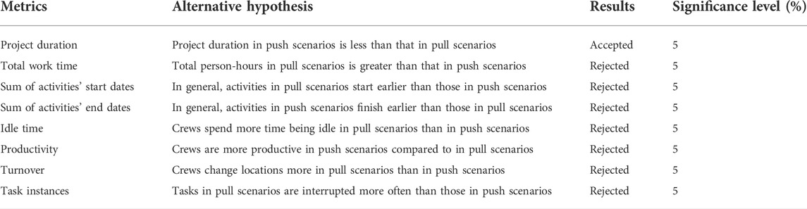
TABLE 3. Hypotheses and their results.
Project duration and flowlines
Project duration is expected to be shorter in push scenarios, because planning focuses on starting tasks as soon as possible. However, considering a pull scenario, project duration can be enhanced if the LBMS plan is optimized through assigning an appropriate aligned production rate to be followed for activities and through reducing time buffers. In this case, the considered pull scenarios started from an aligned location-based plan and both the push and pull plans were planned to finish at the same time.
On average, project duration was shorter in push scenarios than in pull scenarios. However, the difference in average project durations between push and pull approaches was around 14 workdays (376 workdays in push scenarios and 390 workdays in pull scenarios). In other words, pull approaches showed a 3.7% increase in project duration, which is relatively minor.
A main reason push scenarios have shorter project durations is that in a pull scenario, the reference activity, which is used to tell if an activity is late, early, or on time, is the first continuous activity encountered before the activity being studied. Thus, if the reference activity is late and has a milder slope than the predecessor activity, the activity after it will be delayed accordingly, and if this subsequent activity is also delayed (maintaining a continuous flowline), delays in following downstream activities can accumulate, leading to an overall greater project duration.
The flowline displayed in Figure 7 is for a representative run of a pull approach. Figure 8 presents a separate legend for the flowline graphs. The flowlines display continuity for the majority of activities, which means that once crews finish working on a specific task in a location, they continue to work on the same task in the upcoming location. Note that not all crews move in the same location sequence; rather, their movement depends on the utilities/scores generated by the utility function, which determines the most suitable task for each crew based on the schedule, the anticipated productivity in the new location, and the proximity between current and new locations.
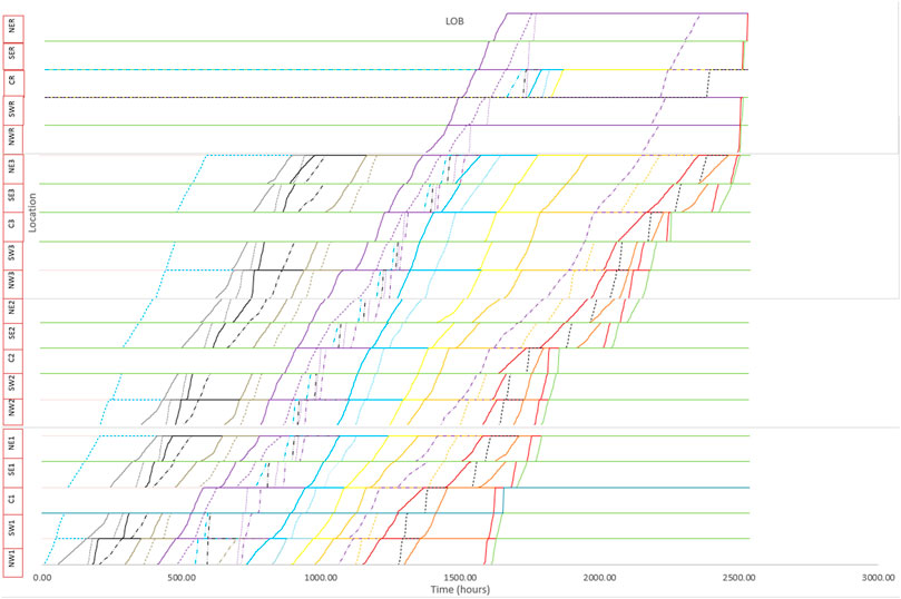
FIGURE 7. Flowline diagram of a representative pull run.
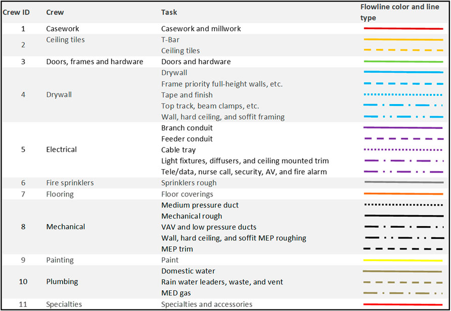
FIGURE 8. Legend for flowline graphs in this paper.
In addition, a task’s flowline may display sharp or gentle slopes for different times. The slope represents production rate, so steep slopes mean high production rates and gentle (flatter) slopes mean low production rates. As explained earlier, the reference that determines what “steep” or “gentle” slopes are is the comparison with the slope of the first continuous activity encountered before it. If the slope is gentler, then the task is delayed, and more crews (up to the maximum number of crews allowed) are allocated to get the task back on track. If it is not possible to add resources to achieve the required production rate without congestion, the pull approach starts work in an unconstrained location (thus breaking the flowline continuity) to achieve the required production rate without congestion. Note that a few tasks had discontinuous flowlines, since they had small quantities to be executed and relatively high production rates for the crews working on them.
A flowline for a representative push scenario is shown in Figure 9, where no continuity exists in the task flowlines. Pointers in Figure 9 indicate some examples of discontinuity. Tasks have multiple interruptions if a crew is working on an activity that is early or on time, another activity is delayed, and as a result this crew may move to that activity (depending on the utilities of those tasks), which leads to a break/interruption in the current activity (shown as a horizontal line in the flowline of this specific activity). So, since many crews are allocated to a late activity (making its production rate high and thus its flowline’s slope steep) and since tasks are not continuous (no link exists between the same activities in different locations), the overall project duration in push scenarios is less than in pull scenarios.
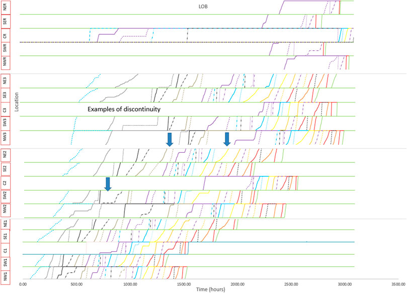
FIGURE 9. Flowline of a representative push run.
Total work time and labor costs
Total work time is the sum of work time for all crews throughout the whole project. On average, crews worked 8,118 cumulative hours in push scenarios but only 5,633 h in pull scenarios. This is a difference of 2,485 h. Throughout all simulations, labor costs increased in push compared to pull scenarios by 29%–31%. This was mainly due to the increased productivity of crews in pull cases; crews may be allocated to late activities in a push scenario regardless of the level of congestion they cause and its effect on productivity. Decreased productivity means each crew works longer to generate the same amount of work. Thus, the sum of all crews’ work times will be greater for push scenarios than pull scenarios.
Production system cost is the cost related to production without considering contractual relationships between parties (i.e., assuming all crews are directly employed) (Kenley and Seppänen 2010). Change in total work time affects production system costs. Push and pull approaches resulted in different total work times required to finish the project. This indicates the production system cost change between these two types of scenarios. For simplicity, an average wage (x dollars/h) was assumed for all crews, which means adopting a pull scenario indicates a decrease in labor costs as follows:
Comparing the metrics of production labour cost and project duration, labor costs are expected to be significantly less in pull scenarios than in push scenarios. However, a project might require slightly more time to finish, increasing overhead costs. This suggests that depending on the actual status of the project, a combination of push and pull approaches can be used for production control.
Sum of activities’ start and end dates
The sum of start dates of all activities for all simulation runs is shown in Figure 10, which shows that activities in push scenarios start earlier on average than in pull scenarios. This is because activities in the pull scenario plan do not start as early as possible, but instead, a task start date is delayed such that a continuous flowline can be maintained according to location-based management principles.
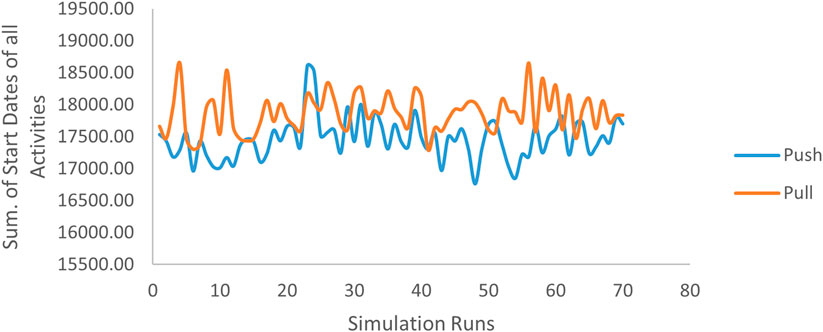
FIGURE 10. Sum of start dates.
The sum of end dates of all activities for all simulation runs is shown in Figure 11, which shows that activities in pull scenarios finish earlier than those in push scenarios. The reason is that in a push scenario, most activities tend to be finished close to the end of the project, making the sum of all end dates a large value. In a pull scenario, even though the total duration of the project is greater than that for a push scenario, activities are more spread out over the course of the project. In other words, some activities finish earlier on in the project lifespan and others finish later, making the total of all end dates less than that for a push scenario.
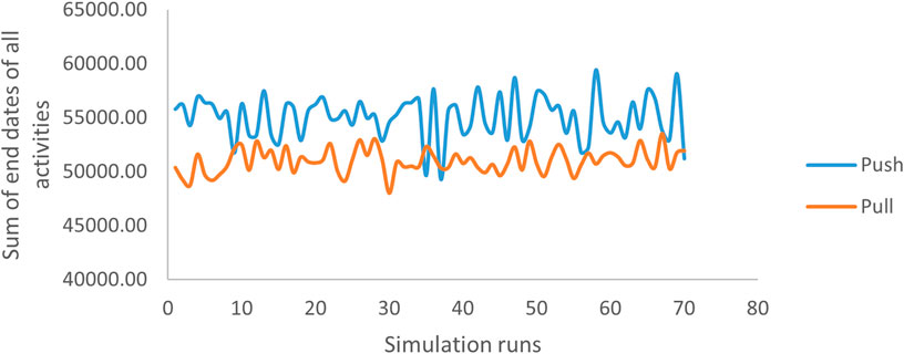
FIGURE 11. Sum of activities’ end dates.
Thus, results for both metrics show that starting activities as early as possible, which is one method of push applications in production control, does not necessarily mean they are finished early. However, starting an activity at the last responsible moment enables continuous work through different locations, which leads to many activities finishing earlier on average than in the push scenario.
Productivity
In general, crew productivity was better for pull scenarios than push scenarios. Figure 12 shows percentage increase in productivity, which varied from 0% for “Specialties” to 47% for “Mechanical.”
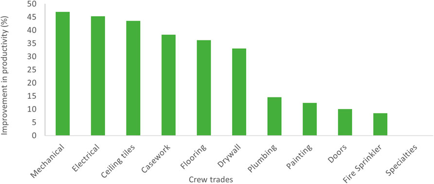
FIGURE 12. Improvement in the average productivity of all crew types from push to pull scenarios.
As described previously, productivity is affected by the level of overstaffing a location; more crews working together means each achieves lower productivity. In push scenarios, all resources available from the contractor can be mobilized to a certain location, while in pull scenarios resources are mobilized only when productivity starts to decrease, at which time they are mobilized to subsequent locations. Thus, in the case of a late task, many crews work together, leading to increased reduction in each crew’s productivity. In pull scenarios, even though an activity is late, additional locations tend to be opened (empty locations pull resources) so productivity is not sacrificed. Therefore, productivity is less affected in a pull scenario compared to a push scenario.
Crews’ productivities improved at different rates; some crews, such as those for “Ceiling tiles,” “Electrical,” and “Mechanical,” showed greater improvements (up to 47%), whereas other crews, such as “Doors” and “Fire sprinklers,” only had 10% improvement. The difference in productivity increases is linked to the number of available crews for each type of work. Trades with a high number of crews showed greater improvements. Trades with little or no improvement included those whose production rates were high and only one crew was on site. In these cases, no pull benefit existed, because the work had to be done discontinuously in any case since it was not possible to slow production to match the production rate of the predecessor task. This suggests that the difference between pull and push control methods may especially manifest in larger scopes of work.
Idle time
Idle time is the time during which a crew is onsite but not working. On real-world construction sites, crews are idle when they are on site but not producing anything that adds value. This is explicitly clarified in the model through distinguishing between “Working” and “Idle” states. These assumptions are aligned with production system cost calculations defined by Kenley and Seppänen (2010).
The percentage of time spent being idle for each crew for all simulation runs for both push and pull scenarios was calculated. Figure 13 presents an average value for each set of crews. Results show that crews spend less time being idle in pull scenarios. This is mainly due to the continuity of tasks between locations in a pull scenario. For example, for a pull scenario where a crew finishes working on a task, this crew has a higher probability of finding another activity to work on, with one option being the same task in the following location, and thus this crew will not spend much time being idle. The flowline presented in Figure 7 clearly shows this, where many tasks start immediately after the same task in the previous location finishes, and thus crews work continuously. In a push scenario, a crew that finishes an activity might not find another activity to work on, at least in terms of the same task in the following location that has a low probability of being unconstrained and being ready to be executed, and thus they must be idle until another activity becomes unconstrained.
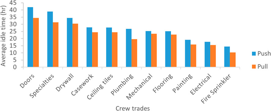
FIGURE 13. Average idle time for all crew types.
Additionally, different crews spent different percentages of their time being idle and therefore show the same behavior (trend) for both push and pull scenarios. The percentage of idle time depends on factors such as the number of tasks worked on by each trade and the proximity of execution times for these tasks. These two factors are not mutually exclusive, as illustrated by considering examples of crews with different idle time percentages, such as “Doors” and “Electrical” crews; “Doors” crews had high percentages of idle time, whereas “Electrical” crews had much lower percentages of the same. Only one task composed of 19 activities is allocated to “Doors” crews, whereas five tasks with a total of 95 activities are assigned to “Electrical” crews. In a case where a task is late and many crews are working on it, additional crews will leave the task once it is back on schedule, going back to their idle state to look for other activities. If no activities are available within one workday, the crews will leave the site. In such a case, “Electrical” crews have a higher probability of finding another concurrent task to work on; thus, they will have little idle time. This phenomenon lease impacts multi-skilled contractors with many different tasks on the project. Single-task contractors with high production rates (e.g., “Doors,” “Specialties”) were most impacted by idle time.
Turnover rate
Turnover rate describes how many locations each crew visits throughout the project lifetime. This metric is measured for each crew in every simulation run. Figure 14 shows an average value for turnover rate for each set of crews.
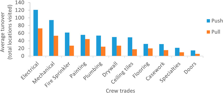
FIGURE 14. Average turnover for all crew types.
As shown in Figure 14, crews changed more locations in push scenarios than in pull scenarios. This is mainly linked to the approaches used to handle late activities. In cases adopting push approaches, a late activity is managed by allocating more crews to it; thus, crews working on activities with lower utilities (activities that are early or on time) will move to the late task, and once it is on time again, they will leave it to go to another activity that is running late, and so on. In pull scenarios, the number of crews that can work on a late activity is limited. This reduces crews’ turnover accordingly, since a late activity with the maximum allowable number of crews working on it will not have a high utility anymore, so crews will not move to it.
Furthermore, different types of crews had varying turnover rates, which is related to the number of tasks allocated to each type of crew and the time span between the execution of these tasks. The more tasks allocated to a crew and the higher the probability of the tasks being executed simultaneously, the greater the likelihood for crews to move from one task to another.
In addition, turnover rate is related to the idle time of crews; crews with high turnover rates had lower idle times (e.g., Electrical) since they had more options (tasks to work on) and a higher probability of performing tasks with higher utilities than the tasks being executed, and thus, the likelihood of changing locations was greater. On the other hand, crews with low turnover rates had greater idle times (e.g., for “Doors” and “Flooring”) due to the limited options they had while idle.
Conclusion and recommendations
Production planning and control are essential construction processes and need to be optimized to achieve successful project outcomes. Many studies have addressed techniques that improve production control, mainly through comparing push and pull planning from a theoretical planning perspective, paying less attention to the effect of these techniques on crew-level decision-making and its impacts on project-level outcomes.
This study evaluated the implementation of the techniques of push and pull production control approaches on project-level outcomes by first conducting a thorough literature review and highlighting research gaps. Next, a conceptual model was developed that depicts push and pull production control approaches at the crew level. AnyLogic was used to develop an agent-based model that represents a construction site with interacting workers. Data was collected for several metrics relating to crews and project performance. These metrics were then compared in push and pull scenarios, and the results were analyzed.
The results of this study show that pull approaches have better results in terms of most of the measured metrics. At the crew level, pull scenarios resulted in higher productivity, less idle time, and lower turnover rates. These results show that pull approaches can enhance overall crew performance, which reduces additional costs and time delays associated with crews’ low productivity and wasted idle time.
At the activity level, it was noted that in pull scenarios, activities generally started later and finished earlier than activities in push scenarios, showing that starting earlier does not necessarily mean finishing earlier. Moreover, fewer work interruptions occurred with tasks in pull scenarios, which ensures a continuous workflow of activities and less fluctuation in the number of tasks executed.
Regarding metrics related to project performance, it was noted that push scenarios led to earlier finish times than pull scenarios but with significantly more person-hours. Work by Kelley and Walker (1959) on CPM modeled activity durations so that shorter durations require “crashing” costs. According to the results of the study presented here, crashing costs may in fact be costs related to push control approaches.
This study showed that both push and pull production control approaches have pros and cons and adopting one approach to control a whole project will not yield optimum results in terms of productivity, idle time, lower turnout rates and project duration. Push and pull scenarios can be used in a complementary, combined fashion. In particular, the greater durations of pull schedules depend on the choice of reference task. In the simulation for this study, the previous continuous task was used, and the planned production rate was used for the first task. A more aggressive assumption could be used. For instance, the reference production rate of the first task could be set to the numerical value required to meet project milestones, which would lead to later tasks having a higher production target. Future research may propose other ways to combine pull and push approaches.
Some limitations of this study include the input of the agent-based model used, which could be further validated through assessing it with respect to different types of construction projects. Also, considering construction logistics, the proposed model assumes continuous supply of material to all locations. Thus, future research can consider the effect of applying push and just-in-time delivery approaches for on-site materials along with push and pull approaches. Finally, the conclusions of this study were based on running the simulation using data from one construction project. Future research investigations could utilize additional projects for further validation.
Data availability statement
The raw data supporting the conclusion of this article will be made available by the authors, without undue reservation.
Author contributions
MG, FH, EZ, and OS contributed to conception and design of the study. MG and EZ developed the simulation model and performed analysis with support from FH and OS. MG wrote the first draft of the manuscript. LS wrote the final draft of the manuscript and helped address the reviewers' comments. All authors wrote sections of the manuscript. All authors contributed to manuscript editing, read, and approved the submitted version.
Funding
This study is partially funded by the Civil Engineering department at American University of Beirut (AUB). It is also partially funded by the Natural Sciences and Engineering Research Council of Canada (NSERC) Alliance grant ALLRP 549210-19.
Conflict of interest
The authors declare that the research was conducted in the absence of any commercial or financial relationships that could be construed as a potential conflict of interest.
Publisher’s note
All claims expressed in this article are solely those of the authors and do not necessarily represent those of their affiliated organizations, or those of the publisher, the editors and thereviewers. Any product that may be evaluated in this article, or claim that may be made by its manufacturer, is not guaranteed or endorsed by the publisher.
Author disclaimer
All findings and conclusions expressed in this paper are those of the authors and do not reflect those of the contributors.
References
Arditi, D., Tokdemir, O. B., and Suh, K. (2002). Challenges in line-of-balance scheduling. J. Constr. Eng. Manag. 128 (6), 545–556. doi:10.1061/(asce)0733-9364(2002)128:6(545)
Ballard, G. (2000). The last planner system of production control. UK: Faculty of Engineerimg, The University of Birmingham. Ph.D. dissertation.
Barakat, M., and Khoury, H. (2016). “An agent-based framework to study occupant multi-comfort level in office buildings,” in Proceedings - Winter Simulation Conference - IEEE (Arlington, Virginia, USA: IEEE), 1328–1339. doi:10.1109/WSC.2016.7822187
Bennett, J. (1991). International construction project management: General theory and practice. Oxford: Butterworth-Heinemann.
Bennett, N. D., Croke, B. F. W., Guariso, G., Guillaume, J. H. A., Hamilton, S. H., Jakeman, A. J., et al. (2013). Characterising performance of environmental models. Environ. Model. Softw. 40, 1–20. doi:10.1016/j.envsoft.2012.09.011
Chen, X., Ong, Y. S., Tan, P. S., Zhang, N. S., and Li, Z. (2013). “Agent-based modeling and simulation for supply chain risk management - a survey of the state-of-the- art,” in 2013 IEEE International Conference on Systems, Man, and Cybernetics (Manchester, United Kingdom: IEEE), 1294–1299. doi:10.1109/SMC.2013.224
Dallasega, P., Marengo, E., and Revolti, A. (2021). Strengths and shortcomings of methodologies for production planning and control of construction projects: A systematic literature review and future perspectives. Prod. Plan. Control 32 (4), 257–282. doi:10.1080/09537287.2020.1725170
Damci, A., Arditi, D., and Polat, G. (2013). Multiresource leveling in line-of-balance scheduling. J. Constr. Eng. Manag. 139 (9), 1108–1116. doi:10.1061/(asce)co.1943-7862.0000716
Dawood, N., and Mallasi, Z. (2006). Construction workspace planning: Assignment and analysis utilizing 4D visualization technologies. Computer-aided Civ. Eng. 21 (7), 498–513. doi:10.1111/j.1467-8667.2006.00454.x
De Toni, A., Caputo, M., and Vinelli, A. (1988). Production management techniques: Push‐pull classification and application conditions. Int. J. Operations Prod. Manag. 8 (2), 35–51. doi:10.1108/eb054818
Eppstein, M. J., Rizzo, D. M., Lee, B. H. Y., Krupa, J. S., and Manukyan, N. (2015). Using national survey respondents as consumers in an agent-based model of plug-in hybrid vehicle adoption. IEEE Access 3, 457–468. doi:10.1109/ACCESS.2015.2427252
Feng, Q., Hai, X., Huang, B., Zuo, Z., Ren, Y., Sun, B., et al. (2019). An agent-based reliability and performance modeling approach for multistate complex human-machine systems with dynamic behavior. IEEE Access 7, 135300–135311. doi:10.1109/ACCESS.2019.2941508
Frandson, A., Seppänen, O., and Tommelein, I. D. (2015). “Comparison between location based management and takt time planning,” in GLC23, 23rd Annual Conference of the International Group for Lean Construction. Perth, Australia, 3–12.
Garcia-Magarino, I., Plaza, I., Igual, R., Lombas, A. S., and Jamali, H. (2020). An agent-based simulator applied to teaching-learning process to predict sociometric indices in higher education. IEEE Trans. Learn. Technol. 13 (2), 246–258. doi:10.1109/TLT.2019.2910067
Gayer, B. D., Saurin, T. A., and Wachs, P. (2021). A method for assessing pull production systems: A study of manufacturing, healthcare, and construction. Prod. Plan. Control 32 (13), 1063–1083. doi:10.1080/09537287.2020.1784484
Ghanem, M., Hamzeh, F., Seppänen, O., and Zankoul, E. (2018). “A new perspective of construction logistics and production control: An exploratory study,” in IGLC26 Proceedings of the 26th Annual Conference of the International Group for Lean Construction (Chennai, India, 992–1001.
Ghosh, S., Reyes, M., Perrenoud, A., and Coetzee, M. (2017). “Increasing the productivity of a construction project using collaborative pull planning,” in Aei 2017: Resilience of the integrated building. Oklahoma City, Oklahoma, USA: ASCE, 825–836.
Hamzeh, F., Al Hattab, M., Rizk, L., El Samad, G., and Emdanat, S. (2019). Developing new metrics to evaluate the performance of capacity planning towards sustainable construction. J. Clean. Prod. 225, 868–882. doi:10.1016/j.jclepro.2019.04.021
Hamzeh, F., Zankoul, E., and Rouhana, C. (2015). How can ‘tasks made ready’ during lookahead planning impact reliable workflow and project duration? Constr. Manag. Econ. 33 (4), 243–258. doi:10.1080/01446193.2015.1047878
Haryadi, F. N., Ali Imron, M., Indrawan, H., and Triani, M. (2019). “Predicting rooftop photovoltaic adoption in the residential consumers of PLN using agent-based modeling,” in 2019 International Conference on Technologies and Policies in Electric Power and Energy, TPEPE - IEEE, 1. Yogyakarta, Indonesia–5. doi:10.1109/IEEECONF48524.2019.9102558
Hopp, W. J., and Spearman, M. L. (2004). To pull or not to pull: What is the question? Manuf. Serv. Oper. Manag. 6 (2), 133–148. doi:10.1287/msom.1030.0028
Hosny, A., Nik-Bakht, M., and Moselhi, O. (2020). Workspace planning in construction: Non-deterministic factors. Automation Constr. 116, 103222. doi:10.1016/j.autcon.2020.103222
Howell, G., Laufer, A., and Ballard, G. 1993. “Interaction between subcycles: One key to improved methods.” J. Constr. Eng. Manag., 119 (4): 714–728. doi:10.1061/(asce)0733-9364(1993)119:4(714)
Kalsaas, B. T., Skaar, J., and Thorstensen, R. T. (2015). “Pull vs. push in construction work informed by last planner,” in IGLC23 23rd Annual Conference of the International Group for Lean Construction. Perth, Australia, 103–112.
Kelley, J. E., and Walker, M. R. (1959). “Critical-path planning and scheduling,” in Proceedings of the Eastern Joint Computer Conference, IRE-AIEE-ACM, 160. Boston, MA, USA: ACM Digital Library–173.
Kenley, R., and Seppänen, O. (2010). Location-based management for construction: Planning, scheduling and control. London and New York: Spon Press.
Knotten, V., Svalestuen, F., Hansen, G. K., and Lædre, O. (2015). Design management in the building process - a review of current literature. Procedia Econ. Finance 21, 120–127. doi:10.1016/s2212-5671(15)00158-6
Lehtovaara, J., Seppänen, O., and Peltokorpi, A. (2022). Improving construction management with decentralised production planning and control: Exploring the production crew and manager perspectives through a multi-method approach. Constr. Manag. Econ. 40 (4), 254–277. doi:10.1080/01446193.2022.2039399
Macal, C. M., and North, M. J. (2011). “Introductory tutorial: Agent-based modeling and simulation,” in Proceedings of the 2011 Winter Simulation Conference (WSC) (Phoenix, AZ, USA: IEEE), 1451–1464. doi:10.1109/WSC.2011.6147864
Olivieri, H., Seppänen, O., and Denis Granja, A. (2018). Improving workflow and resource usage in construction schedules through location-based management system (LBMS). Constr. Manag. Econ. 36 (2), 109–124. doi:10.1080/01446193.2017.1410561
Raoufi, M., and Fayek, A. R. (2015). “Integrating Fuzzy Logic and agent-based modeling for assessing construction crew behavior,” in Annual Conference of the North American Fuzzy Information Processing Society - NAFIPS - IEEE (Redmond, WA, USA: IEEE), 1–6. doi:10.1109/NAFIPS-WConSC.2015.7284151
Robinson, S., Nance, R. E., Paul, R. J., Pidd, M., and Taylor, S. J. E. (2004). Simulation model reuse: Definitions, benefits and obstacles. Simul. Model. Pract. Theory 12 (7–8), 479–494. doi:10.1016/j.simpat.2003.11.006
Sacks, R., and Harel, M. (2006). An economic game theory model of subcontractor resource allocation behaviour. Constr. Manag. Econ. 24 (8), 869–881. doi:10.1080/01446190600631856
Sanders, S. R., and Thomas, H. R. (1991). Factors affecting masonry-labor productivity. J. Constr. Eng. Manag. 117 (4), 626–644. doi:10.1061/(asce)0733-9364(1991)117:4(626)
Sargent, R. G. (2013). Verification and validation of simulation models. J. Simul. 7 (1), 12–24. doi:10.1057/jos.2012.20
Seppänen, O. (2012). “A production control game for teaching of location-based management system’s controlling methods,” in IGLC20 2012 - 20th Conference of the International Group for Lean Construction (San Diego, USA.
Seppänen, O. (2009). Empirical research on the success of production control in building construction projects. Ph.D. dissertation. Espoo (Finland): Helsinki University of Technology.
Seppänen, O., Evinger, J., and Mouflard, C. (2014). Effects of the location-based management system on production rates and productivity. Constr. Manag. Econ. 32 (6), 608–624. doi:10.1080/01446193.2013.853881
Thomas, H. R. (1992). Effects of scheduled overtime on labor productivity. J. Constr. Eng. Manag. 118 (1), 60–76. doi:10.1061/(asce)0733-9364(1992)118:1(60)
Thomas, H. R., Sanvido, V. E., and Sanders, S. R. (1989). Impact of material management on productivity - a case study. J. Constr. Eng. Manag. 115 (3), 370–384. doi:10.1061/(asce)0733-9364(1989)115:3(370)
Tommelein, I. D. (1998). Pull-driven scheduling for pipe-spool installation: Simulation of lean construction technique. J. Constr. Eng. Manag. 124 (4), 279–288. doi:10.1061/(asce)0733-9364(1998)124:4(279)
Trinh, M. T., and Feng, Y. (2020). Impact of project complexity on construction safety performance: Moderating role of resilient safety culture. J. Constr. Eng. Manag. 146 (2), 04019103. doi:10.1061/(ASCE)CO.1943-7862.0001758
Keywords: production planning and control, pull planning, push planning, crew performance, location-based management, agent-based modelling
Citation: Ghanem M, Hamzeh F, Seppänen O, Shehab L and Zankoul E (2022) Pull planning versus push planning: Investigating impacts on crew performance from a location-based perspective. Front. Built Environ. 8:980023. doi: 10.3389/fbuil.2022.980023
Received: 28 June 2022; Accepted: 05 September 2022;
Published: 03 October 2022.
Edited by:
Shang Gao, The University of Melbourne, AustraliaReviewed by:
Søren Wandahl, Aarhus University, DenmarkYanqing Fang, Tianjin University of Finance and Economics, China
Copyright © 2022 Ghanem, Hamzeh, Seppänen, Shehab and Zankoul. This is an open-access article distributed under the terms of the Creative Commons Attribution License (CC BY). The use, distribution or reproduction in other forums is permitted, provided the original author(s) and the copyright owner(s) are credited and that the original publication in this journal is cited, in accordance with accepted academic practice. No use, distribution or reproduction is permitted which does not comply with these terms.
*Correspondence: Farook Hamzeh, aGFtemVoQHVhbGJlcnRhLmNh