Probabilistic Identification of Multi-DOF Structures Subjected to Ground Motion Using Manifold-Constrained Gaussian Processes

Bayesian uncertainty quantification has a pivotal role in structural identification, yet the posterior distribution estimation of unknown parameters and system responses is still a challenging task. This study explores a novel method, named manifold-constrained Gaussian processes (GPs), for the probabilistic identification of multi-DOF structural dynamical systems, taking shear-type frames subjected to ground motion as a demonstrative paradigm. The key idea of the method is to restrict the GPs (priorly defined over system responses) on a manifold that satisfies the equation of motion of the structural system. In contrast to widely used Bayesian probabilistic model updating methods, the manifold-constrained GPs avoid the numerical integration when formulating the joint probability density function of unknown parameters and system responses, hence achieving an accurate and computationally efficient inference for the posterior distributions. An eight-storey shear-type frame is analyzed as a case study to demonstrate the effectiveness of the manifold-constrained GPs. The results indicate the posterior distributions of system responses, and unknown parameters can be successfully identified, and reliable probabilistic model updating can be achieved.

1 Introduction

The identification of structural systems, formulated as an inverse problem, refers to any systematic way of updating the model of a structure through the use of experimental data. The main purpose of structural identification is to correlate the model and the real system for the purpose of, for example, reliable estimates of performance and vulnerability of the structural system in service (Catbas et al., 2013). In the past decades, numerous structural identification techniques leveraging vibration measurements have been proposed and successfully applied to real-world civil engineering structures. These methods utilize either time-domain or frequency-domain observations (and input-output or output-only data) to inversely map the monitored data onto the corresponding structural parameters, and the parameters can be further used to predict structural response to future dynamic loads or assess the structural conditions (Sun and Betti, 2013). In time-domain identification methods, the difference in vibration responses (e.g., acceleration, velocity, displacement, and strain) between the parameterized model and the real system is directly evaluated. Some innovative methods using (incomplete) output-only time-domain data to identify structural parameters and input force have been developed by Chen and Li (2004), Lu and Law (2007), Sandesh and Shanker (2009), and Sun and Betti (2013). By contrast, the input-output–related methods executed in the time domain could be more intuitive and robust to apply, although more sensor cost would be demanded in the monitoring system. Several researchers have explored input-output–related time-domain methods, such as Behmanesh and Moaveni (2014) and Lei et al. (2019). In frequency-domain identification methods, modal properties such as natural frequencies (Hassiotis and Jeong, 1995), mode shapes (Morassi and Tonon, 2008), frequency response function (Ni et al., 2006; Zhou and Tang, 2021a), and modal strain energy (Shi et al., 2002) are extracted from measured dynamic response data of a structure of interest, and the discrepancies between the identified and model-derived modal properties are utilized for model updating and structural condition assessment. In this study, the structural responses and unknown parameters will be estimated using time-domain data.

As is often the case during the monitoring of structures, uncertainties from various sources exist in the monitored data, making the identification results unreliable or even leading to false results (Beck and Yuen, 2004). Hence, a probabilistic way of structural identification is desirable for many problems. It is well known that the Bayesian methods enable addressal of the uncertainties in structural identification, which account for various sources of uncertainties observed in the real world. Numerous research works have been conducted in pursuit of Bayes’ theorem to compute the posterior distributions of either structural responses or unknown parameters. The traditional methods, such as Bayesian Kalman filters, particle filters, and Markov chain Monte Carlo, are widely applied for the sampling-based inference of posterior distributions (Behmanesh and Moaveni, 2014; Capellari et al., 2015; Li et al., 2016). Ramancha et al. (2020) presented a sequential Monte Carlo method to update a nonlinear finite element model of a full-scale reinforced-concrete bridge subjected to seismic excitations. Parallel model evaluation is a remarkable advantage of the sequential Monte Carlo, which is ideal for updating computationally expensive models. Behmanesh et al. (2015) proposed a hierarchical Bayesian modeling technique for probabilistic finite element model updating, which predicts uncertainty in parameter estimation and captures the inherent time-variability of structural parameters as well. Sun and Betti (2015) proposed a hybrid optimization methodology to implement Bayesian inference in model updating, which could be effectively applied to determine the unknown system parameters and uncertainties over the parameters using a weighted sum of Gaussian distributions. Erazo and Nagarajaiah (2018) applied unscented Kalman filtering to estimate the parameters that define the nonlinear models of structures equipped with negative stiffness systems. Huang et al. (2017) proposed a hierarchical sparse Bayesian learning and Gibbs sampling algorithm to estimate the high-dimensional uncertain parameters which arise from sparse stiffness identification problems. Rocchetta et al. (2018) developed an efficient and robust procedure within the Bayesian model updating framework to detect crack location and size in mechanical components, where an emulator was generated as a substitution for the finite element model to reduce the computational cost and enable on-line Bayesian model updating. Kamariotis et al. (2022) developed a Bayesian model updating–based method to sequentially learn structural deterioration and estimate structural damage evolution over time. Adeagbo et al. (2021) pursued railway ballast damage identification by exploring a time-domain Markov chain Monte Carlo–based Bayesian model updating method, in which a novel stopping criterion was proposed to correctly identify the scaling factors of the system properties.

The GP-based Bayesian modeling is another attractive topic in the Bayesian community, which generally simplifies the priors to be Gaussian and thus effectively alleviates the high-computational cost faced by other Bayesian methods. A multi-task GP method was developed by Wan and Ni (2019) to reconstruct missing structural health monitoring data; specifically, the method enables the modeling of a series of tasks simultaneously. Wan and Ni (2018) presented a moving-window strategy to achieve a reduced-order GP model, which has been effectively used to forecast structural stress responses. Zhou and Tang (2018) proposed a framework based on the combination of a two-level GP emulator and Bayesian inference. The framework employed multi-fidelity data from a full-scale finite element model and a component mode synthesis reduced-order model, which has been successfully applied to update the key parameters of a structural system. Xue et al. (2020) explored the system identification of a ship dynamic model in terms of an improved GP regression algorithm. A mode shape uncertainty quantification approach was proposed by Zhou and Tang (2021b) by using a multi-response GP meta-modeling strategy, which demonstrated computation efficiency for uncertainty quantification of mode shapes at multiple locations. The aforementioned studies have demonstrated the strong capability of GPs in the framework of Bayesian inference and meanwhile, provided new thoughts on probabilistic structural identification.

This study pursues a novel manifold-constrained GP approach (Yang et al., 2021) to estimate the joint posterior distribution of unknown structural parameters and dynamical responses. The equation of motion of a shear-type frame structure subjected to ground motion is addressed in the state space. The GP prior is pre-imposed over each system state, explicitly conditioned on a manifold constraint that the derivative of the GPs must satisfy the equation of motion of the structure. The idea behind it is that the probability density function of any multivariate Gaussian distribution has a closed-form expression (Rasmussen and Williams, 2006); whereas, for other types of joint distribution, high-dimensional integration would be inevitable in the formulation. By leveraging the manifold-constrained GPs, the joint posterior distribution of the system state and unknown parameters are decomposed as the multiplication of several multivariate Gaussian distributions and the prior of the unknown parameters, so that the Hamiltonian Monte Carlo method (Neal, 2010) can be effectively implemented to generate samples from the system state which finally makes the samples’ distribution converge to the target posterior distribution. In comparison with other Bayesian methods to conduct probabilistic identification, the advantage of the manifold-constrained GPs is completely avoiding the high-dimensional integration when formulating the posterior distribution function, thus enhancing the inference accuracy and computational efficiency.

This study is organized as follows. Section 2 elucidates the general methodology of the manifold-constrained GPs in application to multi-DOF structures subjected to ground motion. Section 3 provides a case study on an eight-storey shear-type building to explore the efficacy of the proposed method, from which the results show that the posterior distribution of the unknown structural parameters and system state can be successfully identified under different levels of noise. Conclusions are drawn in Section 4.

2 Basic Formulations

2.1 Gaussian Process

Let X be a variable set and $f:X\to \mathrm{ℝ}$ be a random function. The $f$ is defined as a GP, that is, $f\sim \mathcal{G}\mathcal{P}(\mu ,k)$, where for any $n$ and any finite set of points $\mathit{x}\in X^n$, the random vector $\mathit{f}=f\left(\mathit{x}\right)$ follows a multivariate Gaussian distribution with the mean vector $\mathit{\mu }=\mu \left(\mathit{x}\right)\in {\mathrm{ℝ}}^n$ and covariance matrix ${\mathit{K}}_{\mathit{xx}}=k(x,x)$ (Rasmussen and Williams, 2006).

We assumed that a set of label pairs $(x_i,y_i)$ of $i=1, 2, \mathrm{...}, n$ are observed from the unknown mapping $f:X\to \mathrm{ℝ}$. For the sake of brevity, we denoted $\stackrel{\mathit{ˆ}}{\mathit{x}}={\left(x_1,x_2,\dots ,x_n\right)}^T\in X^{n\times 1}$ and $\stackrel{\mathit{ˆ}}{\mathit{y}}={\left(y_1,y_2,\dots ,y_n\right)}^T\in {\mathrm{ℝ}}^{n\times 1}$. Given that $f\sim \mathcal{G}\mathcal{P}(\mu ,k)$, the joint distribution of the response variable $f\left(x\right)$ associated with the observations $\stackrel{\mathit{ˆ}}{\mathit{y}}$ would follow multivariate Gaussian distribution. According to Bayes’ theorem, the conditional probability density of $f\left(x\right)|\stackrel{\mathit{ˆ}}{\mathit{y}}$ is also a Gaussian distribution $N(\epsilon \left(x\right),\sigma \left(x\right))$. Its mean and variance are given by

$\epsilon \left(x\right)=\mathit{K}\left(x,\stackrel{\mathit{ˆ}}{\mathit{x}}\right)\mathit{K}{\left(\stackrel{\mathit{ˆ}}{\mathit{x}},\stackrel{\mathit{ˆ}}{\mathit{x}}\right)}^{-1}\stackrel{\mathit{ˆ}}{\mathit{y}},(1)$

$\sigma \left(x\right)=\mathit{K}\left(x,x\right)-\mathit{K}{\left(x,\stackrel{\mathit{ˆ}}{\mathit{x}}\right)}^{\mathit{T}}\mathit{K}{\left(\stackrel{\mathit{ˆ}}{\mathit{x}},\stackrel{\mathit{ˆ}}{\mathit{x}}\right)}^{-1}\mathit{K}\left(x,\stackrel{\mathit{ˆ}}{\mathit{x}}\right),(2)$

where $\mathit{K}\left(x,x\right)=k\left(x,x\right)\in \mathrm{ℝ}$, $\mathit{K}\left(x,\stackrel{\mathit{ˆ}}{\mathit{x}}\right)=k(x,\stackrel{\mathit{ˆ}}{\mathit{x}})\in {\mathrm{ℝ}}^{n\times 1}$, and $\mathit{K}\left(\stackrel{\mathit{ˆ}}{\mathit{x}},\stackrel{\mathit{ˆ}}{\mathit{x}}\right)=k\left(\stackrel{\mathit{ˆ}}{\mathit{x}},\stackrel{\mathit{ˆ}}{\mathit{x}}\right)\in {\mathrm{ℝ}}^{n\times n}.$ It is worth mentioning that without loss of generality, the formulations of Eqs 1, 2 are based on the presetting of the mean function $\mu$ in the GP prior on $f$ to being zero. The positive definite kernel function $k: X\times X\to \mathrm{ℝ}$ is properly determined (reflecting the prior knowledge on the properties of the unknown mapping to be approximated, for example, regularity, monotonicity, and periodicity) and parametrized by a vector $\mathit{\theta }$. The determination of the “best-fitted” parameters $\mathit{\theta }$ is made by maximizing the marginal density function, which is given by a high-dimensional intimidating integral $\underset{\widehat{\mathit{x}}}{\overset{ }{{\displaystyle \int }}}p(y\oplus \stackrel{\mathit{ˆ}}{\mathit{y}})\text{d}\stackrel{\mathit{ˆ}}{\mathit{x}}$. Here, the notation $\oplus$ denotes the concatenation of $y$ and $\stackrel{\mathit{ˆ}}{\mathit{y}}$. While one could conceivably perform the high-dimensional integration directly, there exists a closed-form formulation of the integral if $y\oplus \stackrel{\mathit{ˆ}}{\mathit{y}}$ conforms to a multivariate Gaussian distribution, that is, the probability density function of the marginal distribution $p\left(\stackrel{\mathit{ˆ}}{\mathit{y}}\right)$ is given by

$p\left(\stackrel{\mathit{ˆ}}{\mathit{y}}\right)=\text{exp}\left\{-\frac{1}{2}\left[n\text{log}\left(2\pi \right)+\text{log}\left|\mathit{K}(\stackrel{\mathit{ˆ}}{\mathit{x}},\stackrel{\mathit{ˆ}}{\mathit{x}})\right|+{\stackrel{\mathit{ˆ}}{\mathit{y}}}^T\mathit{K}{(\stackrel{\mathit{ˆ}}{\mathit{x}},\stackrel{\mathit{ˆ}}{\mathit{x}})}^{-1}\stackrel{\mathit{ˆ}}{\mathit{y}}\right]\right\}(3)$

In the implementation of GP regression, gradients of the marginal likelihood in Eq. 3 with respect to all unknown parameters $\mathit{\theta }$ are initially derived. By using a gradient-based optimizer with randomized initial guesses, the best-fitted parameters $\mathit{\theta }$ can be estimated. Here, we must emphasize that the reason why GP-based methods are widely adopted in science and engineering is because of the mathematical trick that completely avoids using numerical integration for the calculation of marginal likelihood, but instead gives a concise closed-form mathematical formulation. In the manifold-constrained GPs, this property will be further elaborated for the inference and characterization of uncertainties in parameters that govern the dynamical systems.

2.2 Manifold-Constrained GPs for Structural Dynamical Systems

Consider a discrete $N$-DOF linear system subjected to ground motion, the equation of motion in the state space form is given by

$\dot{\mathit{z}}\left(t\right)\mathrm{=}{\mathbf{A}}_c\mathit{z}\left(t\right)+{\mathbf{B}}_c{a}_g\left(t\right),(4)$

in which the state vector $\dot{\mathit{z}}\left(t\right)$ amounts to ${\left[\mathit{x}\left(t\right),\dot{\mathit{x}}\left(t\right)\right]}^T$ and

${\mathbf{A}}_c=\left[\begin{array}{cc}\mathbf{0}& \mathbf{I}\\ -{\mathbf{M}}^{-1}\mathbf{K}& -{\mathbf{M}}^{-1}\mathbf{C}\end{array}\right]\mathrm{and}{\mathbf{B}}_c=\left[\begin{array}{l}\mathbf{0}\hfill \\ \mathbf{J}\hfill \end{array}\right],(5)$

where ${\mathbf{A}}_c$ is a matrix of the order $2N\times 2N;\mathbf{M},\mathbf{C},\mathbf{K}$ are the mass, damping, and stiffness matrices, respectively, each being of order $N\times N;\mathbf{I}$ is the identity matrix; ${\mathbf{B}}_c$ is a vector of order $2N\times 1$; $\mathbf{J}$ is an $N\times 1$ all-ones vector; and $a_g\left(t\right)$ is the ground acceleration induced by earthquake. In this study, the Rayleigh damping assumption is employed to describe the energy dissipation mechanism of the system, which is expressed as a linear combination of the mass and stiffness matrices in Eq. 6

$\mathit{C}=a\mathit{M}+b\mathit{K},(6)$

where $a$ and $b$ are two constant coefficients that can be derived from

${\xi }_i=\frac{a}{2{\omega }_i}+\frac{b{\omega }_i}{2},(7)$

where ${\xi }_i$ and ${\omega }_i$ are, respectively, the modal damping ratio and natural frequency of the $i^{th}$ vibration mode.

The goal of performing the manifold-constrained GPs for structural dynamical systems is to probabilistically identify damping and stiffness parameters $\left\{a,b,k_1,k_2,\dots ,k_n\right\}$ and the system state, given the information of mass matrix, noise-corrupted observations of displacement, and velocity responses at each DOF and ground acceleration. To this aim, GP prior over $\mathit{z}\left(t\right)$ is initially imposed. A salient feature of GPs is that the derivative of a GP is still a GP with its mean and covariance function completely specified (Raissi et al., 2017). Meanwhile, given Eq. 4, the derivative of $\mathit{z}\left(t\right)$ can also be obtained via the binary operation parametrized by the system parameters. Here, we denote the binary operation as $\mathbf{f}\left(\mathit{z}\left(t\right),\mathit{\varphi },a_g\left(t\right),t\right)$, in which $\mathit{\varphi }$ = ${\left[a,b,k_1,k_2,\dots ,k_N\right]}^T$ is the vector containing damping and stiffness parameters. The key idea is to find a coherent way to deal with the incompatibility of $\dot{\mathit{z}}\left(t\right)$ generated from two distinct sources, that is, data aspect and physical aspect. On the data aspect, $\dot{\mathit{z}}\left(t\right)$ is a set of GPs generated as the derivative of $\mathit{z}\left(t\right)$; on the physical aspect, $\dot{\mathit{z}}\left(t\right)$ is the solution of ordinary differential equations which govern the system dynamics. Hence, a random variable $W$ that quantifies the difference between the two aspects is defined as

$W=\begin{array}{cc}\underset{t\in \mathit{L},d\in \{\mathrm{1,2},\dots ,N\}}{\text{max}}& \left|{\dot{\mathit{z}}}_d\left(t\right)\mathrm{-}{\mathbf{f}}_d\left(\mathit{z}\left(t\right),\mathit{\varphi },a_g\left(t\right),t\right)\right|\end{array},(8)$

where $\mathit{L}=\left\{t_1,t_2,\dots ,t_n\right\}$ denotes a uniform time grid. If the set of GPs on the manifold satisfies the ordinary differential equations, one would obtain $W=0$. Then, the inference over the posterior of the parameters and system state provided the observations of displacement response is of the form

$p(\mathit{\varphi },\mathit{z}\left(\mathit{L}\right)\mathrm{\mid }W=0,\stackrel{\mathit{ˆ}}{\mathit{x}}\left(\mathit{\tau }\right)),(9)$

where for simplicity, we denote $\mathit{z}\left(\mathit{L}\right)$ as the system state containing displacement and velocity responses with respect to the time points in $\mathit{L};\stackrel{\mathit{ˆ}}{\mathit{x}}\left(\mathit{\tau }\right)$ as the noisy observations of displacement responses at time points in $\mathit{\tau }\subseteq \mathit{L}$. Applying Bayes’ theorem, we have

$p(\mathit{\varphi },\mathit{z}\left(\mathit{L}\right)\mathrm{\mid }W=0,\stackrel{\mathit{ˆ}}{\mathit{x}}\left(\mathit{\tau }\right))\propto p(W=0,\stackrel{\mathit{ˆ}}{\mathit{x}}\left(\mathit{\tau }\right),\mathit{z}\left(\mathit{L}\right),\mathit{\varphi }).(10)$

The term on the right-hand side can be decomposed as

$\begin{array}{rr}\hfill p(W=0,\stackrel{\mathit{ˆ}}{\mathit{x}}\left(\mathit{\tau }\right),\mathit{z}\left(\mathit{L}\right),\mathit{\varphi })=& \hfill p\left(\mathit{\varphi }\right)\times p\left(\mathit{z}\left(\mathit{L}\right)\mathrm{\mid }\mathit{\varphi }\right)\times p(\stackrel{\mathit{ˆ}}{\mathit{x}}\left(\mathit{\tau }\right)\mathrm{\mid }\mathit{z}\left(\mathit{L}\right),\mathit{\varphi })\\ \hfill & \hfill \times p(W=0\mathrm{\mid },\stackrel{\mathit{ˆ}}{\mathit{x}}\left(\mathit{\tau }\right),\mathit{z}\left(\mathit{L}\right),\mathit{\varphi })\end{array}.(11)$

Here, the first term $p\left(\mathit{\varphi }\right)$ is specifically determined as a general prior distribution of system parameters. The second term can be simplified as $p\left(\mathit{z}\left(\mathit{L}\right)\right)$ due to the prior independent correlations between the system state $\mathit{z}\left(\mathit{L}\right)$ and system parameters $\mathit{\varphi }$. As we have initially imposed the GP prior over each channel of the system state, $p\left(\mathit{z}\left(\mathit{L}\right)\right)$ can be obtained via the multiplication of the marginal distribution of each multivariate Gaussian distribution in $\mathit{z}\left(\mathit{L}\right)$. The third term, equal to $p\left(\stackrel{\mathit{ˆ}}{\mathit{x}}\left(\mathit{\tau }\right)\mathrm{\mid }\mathit{z}\left(\mathit{L}\right)\right)$, corresponds to the noisy observations. The fourth term can be simplified as $p\left(\dot{\mathit{z}}\left(\mathit{L}\right)=\mathbf{f}\left(\mathit{z}\left(\mathit{L}\right),\mathit{\varphi },a_g\left(\mathit{L}\right),\mathit{L}\right)\mathrm{\mid }\mathit{z}\left(\mathit{L}\right)\right)$, which is the conditional probability of $\dot{\mathit{z}}\left(\mathit{L}\right)$ given $\mathit{z}\left(\mathit{L}\right)$ evaluated at $\mathbf{f}\left(\mathit{z}\left(\mathit{L}\right),\mathit{\varphi },a_g\left(\mathit{L}\right),\mathit{L}\right)$. Recall that ${\dot{\mathit{z}}}_i\left(\mathit{L}\right),i=\mathrm{1,2},\dots ,N$ follows a multivariate Gaussian distribution as the derivative of a GP is still Gaussian. Likewise, $p\left(\dot{\mathit{z}}\left(\mathit{L}\right)=\mathbf{f}\left(\mathit{z}\left(\mathit{L}\right),\mathit{\varphi },a_g\left(\mathit{L}\right),\mathit{L}\right)\mathrm{\mid }\mathit{z}\left(\mathit{L}\right)\right)$ can be formulated as the multiplication of the marginal distribution of each multivariate Gaussian distribution as well (Yang et al., 2021). As illustrated in Eq. 3, the marginal distribution of a multivariate Gaussian distribution eschews the calculation of high-dimensional integral with respect to each random variable in the distribution and instead provides a concise closed-form mathematical formulation. In Eq. 11, the last three terms are Gaussian, thus the following practically computable posterior distribution can be elicited:

$\begin{array}{c}p(\mathit{\varphi },\mathit{z}\left(\mathit{L}\right)\mathrm{\mid }W=0,\widehat{\mathit{x}}\left(\mathit{\tau }\right))\\ \propto p\left(\mathit{\varphi }\right)\times \text{exp}\mathrm{\{}-\frac{1}{2}{\displaystyle \sum }_{i=1}^N[n\text{log}\left(2\pi \right)+\text{log}\left|{\mathit{C}}_i\right|+{\mathit{z}}_i{\left(\mathit{L}\right)}^T{\mathit{C}}_i{\mathit{z}}_i\left(\mathit{L}\right)\end{array}$

$\begin{array}{c}+n\log \left(2\pi \right)+\log \left|{\mathit{G}}_{\mathit{i}}\right|+{\left({\widehat{\mathit{x}}}_{\mathit{i}}\left(\mathit{\tau }\right)-{\mathit{z}}_{\mathit{i}}\left(\mathit{\tau }\right)\right)}^T{\mathit{G}}_{\mathit{i}}\left(\widehat{\mathit{x}}\left(\mathit{\tau }\right)-{\mathit{z}}_{\mathit{i}}\left(\mathit{\tau }\right)\right)\\ +n\log \left(2\pi \right)+\log \left|{\mathit{H}}_i\right|+{{\displaystyle \mathit{q}}}_i^T{\mathit{H}}_i{\mathit{q}}_i\left]\right\},\end{array}(12)$

in which the components ${\mathit{C}}_i,{\mathit{G}}_i,{\mathit{H}}_i$ and ${\mathit{q}}_i$ are, respectively,

$\begin{array}{c}{\mathit{C}}_{\mathit{i}}=c_{\mathit{i}}(\mathit{L},\mathit{L})\\ {\mathit{G}}_i={\sigma }_i(\mathit{L},\mathit{L})\\ {\mathit{H}}_i=c_i″(\mathit{L},\mathit{L})-\prime c_i(\mathit{L},\mathit{L})c_i{(\mathit{L},\mathit{L})}^{-1}{c}_i\prime (\mathit{L},\mathit{L})\\ {\mathit{q}}_i= \prime c_i(\mathit{L},\mathit{L})c_i{(\mathit{L},\mathit{L})}^{-1}{\mathit{z}}_i\left(\mathit{L}\right)-{\mathbf{f}}_i\left(\mathit{z}\left(\mathit{L}\right),\mathit{\varphi },a_g\left(\mathit{L}\right),\mathit{L}\right),\end{array}(13)$

where $\prime c_i=\frac{\partial c_i}{\partial t}\left(t,t\prime \right),c_i\prime =\frac{\partial c_i}{\partial t\prime }\left(t,t\prime \right)$, and $c_i″=\frac{{\partial }^2{c}_i}{\partial t\partial t\prime }\left(t,t\prime \right)$. In this study, the kernel function $c$ is determined as Matern kernel $\mathcal{K}\left(t,t\prime \right)={\kappa }_1\frac{2^{1-\nu }}{\text{Γ}\left(\nu \right)}{\left(\sqrt{2\nu }\frac{l}{{\kappa }_2}\right)}^{\nu }{B}_{\nu }\left(\sqrt{2\nu }\frac{l}{{\kappa }_2}\right)$, where ${\kappa }_1$ and ${\kappa }_2$ are two hyper-parameters; $l=\left|t-t\prime \right|$; $\text{Γ}$ is the Gamma function; $B_v$ is the modified Bessel function of the second kind; and $\nu$ is set to be $2.01$ to enable the kernel to be second-order differentiable (Rasmussen and Williams, 2006). With Eq. 12, the Hamiltonian Monte Carlo method (Neal, 2010) can be applied to generate the samples of the system state $\mathit{z}\left(\mathit{L}\right)$ and parameters $\mathit{\varphi }$, and the samples would quickly converge to being distributed as the target posterior distribution $p(\mathit{\varphi },\mathit{z}\left(\mathit{L}\right)\mathrm{\mid }W=0,\stackrel{\mathit{ˆ}}{\mathit{x}}\left(\mathit{\tau }\right))$. As a summary of the methodology, the flowchart of the manifold-constrained GPs with embedded Hamiltonian Monte Carlo is shown in Figure 1.

FIGURE 1

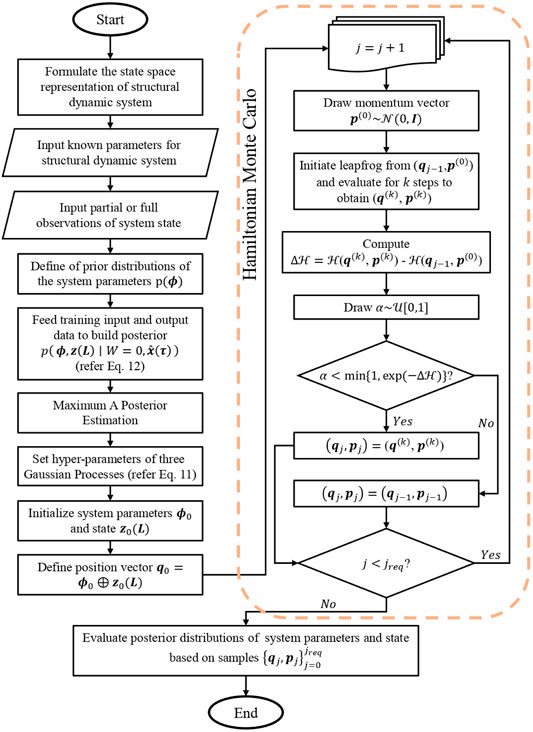
FIGURE 1. Flowchart of the manifold-constrained GPs with embedded Hamiltonian Monte Carlo.

3 Results

An eight-storey building simplified as a shear-type frame structure with masses lumped at each floor is shown in Figure 2. The simplified model has eight DOFs in the horizontal direction. First, it is assumed that there are nine accelerometers instrumented, eight being mounted on the structure and one on the ground. The total displacement and velocity at each DOF and at the ground are obtained by integrating the collected acceleration data series, and the relative displacement and velocity of each floor with respect to the ground could be computed according to the relationship $x_t=x_r+x_g$, where $x_t$, $x_r$, and $x_g$ are the total displacement, relative displacement, and ground displacement, respectively. Parameters of the system are given in Table 1. The first four natural frequencies are 2.77, 7.75, 12.49, and 16.70 Hz. The two Rayleigh constants a and b are, respectively, specified to be 0.20 and 0.01, providing the first two modes of vibration with an approximately 5% damping ratio. The ground motion as external excitation is input into the structural dynamical system in the form of seismic acceleration time history (1995 Kobe Japan earthquake with its peak ground acceleration being scaled to 0.06 g). The dynamic response of each DOF is computed via the fourth-order Runge–Kutta method using a constant time step of 0.01 s. The results are proven to be stable and accurate under the variation of the time step. The generated “measurement” responses with different levels of noise corruption are used to identify the structural dynamical systems in a probabilistic manner. An advantage of the manifold-constrained GPs is that this method can handle uncertainties associated with observations and the model itself. The results not only inform the estimated system state or unknown parameters but also help to understand the credibility of results in practical structural health monitoring (SHM) applications. Before applying the manifold-constrained GPs to the 8-DOF shear-type structure, the input responses and ground acceleration are divided into batches of data, each batch of data containing 50 signal points. It is worth mentioning that the number of discretization points can be greater than 50 as illustrated in Eq. 10, where $\mathit{\tau }\subset \mathit{L}$; in this example, the extent of discretization is determined by gradually increasing the denseness of points until the estimated results “converge.” Then, probabilistic identification is performed fragment by fragment, with the posterior distributions of the system state and stiffness and damping parameters computed by the Hamiltonian Monte Carlo method.

FIGURE 2

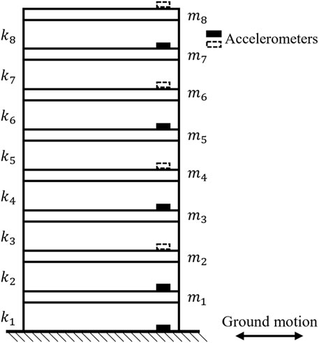
FIGURE 2. An 8-DOF shear-type frame structure with sensors deployed.

TABLE 1

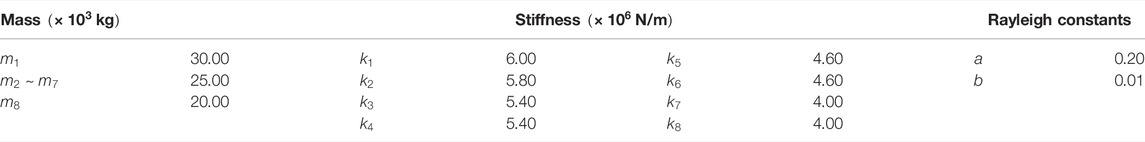
TABLE 1. Structural parameters of the 8-DOF shear-type frame structure.

Figure 3 shows a fragment of the identified displacement and velocity of the third floor under different levels of noise corruption, namely, 0, 5, and 10% root mean square white noise added to the original observations. The identified results fit well with the correct displacement and velocity responses. With the noise level getting higher, the identified confidence intervals generally become wider. Figure 4 elucidates the histograms of the estimated stiffness and damping parameters using the manifold-constrained GPs. Each histogram is generated over 100 parameter sets in the simulation process of the Hamiltonian Monte Carlo, where 0, 5, and 10% root mean square white noise is, respectively, added to the original observations. For computational efficiency, the stiffness and damping parameters are normalized by default. It is seen that the results rigorously reflect the uncertainty over the parameters, for instance, the uncertainty indicated by the blue histogram is greater than that in the green and red histograms which are obtained from observations with lower noise levels. It is noted that the uncertainties on the damping constants a and b are higher than those on the stiffness parameters under the same noise corruption level. This is possibly because the damping constants are more sensitive than the stiffness parameters to noise. The input responses computed by the fourth-order Runge–Kutta method may initially pose noise to the estimation process, especially in the case of ground motion with relatively high frequencies.

FIGURE 3

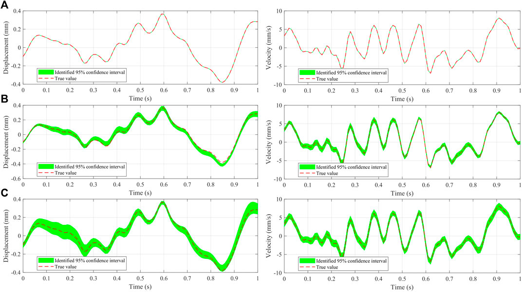
FIGURE 3. Identified displacement and velocity fragments of the third floor under three levels of noise corruption. (A) 0% noise corruption. (B) 5% noise corruption. (C) 10% noise corruption. The red dotted line denotes the true trajectory. The green area represents the identified 95% confidence interval.

FIGURE 4

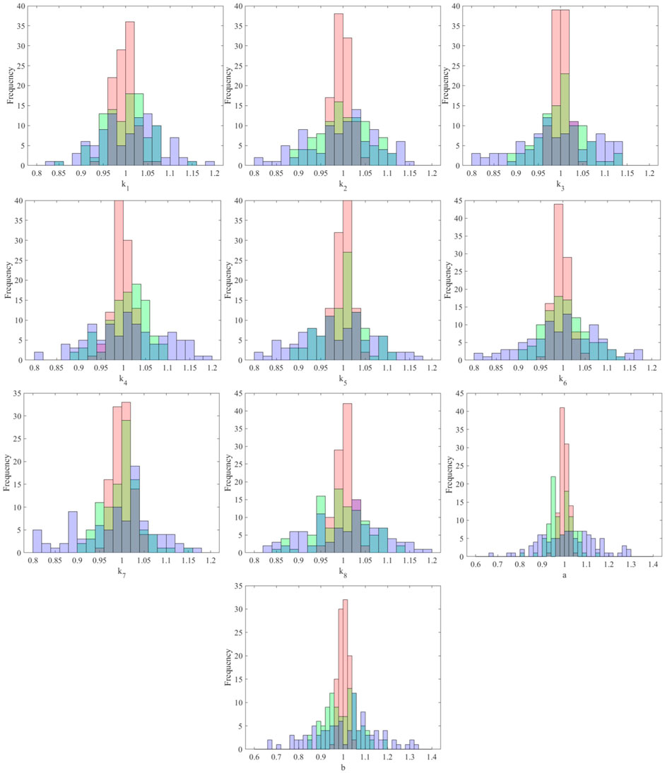
FIGURE 4. Histograms of estimated normalized stiffness and damping parameters over 100 simulated parameter sets under three levels of noise corruption. Red: 0% noise corruption. Green: 5% noise corruption. Blue: 10% noise corruption. The vertical black line is the true parameter value.

According to the basic formulation of the proposed method, the joint posterior distributions of structural parameters and responses under the condition of $\stackrel{\mathit{ˆ}}{\mathit{x}}\left(\mathit{\tau }\right)$ and $W=0$ are elicited. In principle, $\stackrel{\mathit{ˆ}}{\mathit{x}}\left(\mathit{\tau }\right)$ does not need to be all observations of the structural responses. But intuitively, with fewer observations involved to build the posterior in Eq. 12, more uncertainties would arise in the output. Hence, to further verify the performance of manifold-constrain GPs when the structural responses are partially observed, we then assume fewer accelerometers instrumented on the structure. The instrumentation scheme is shown in Figure 2, where the black rectangles denote the locations of accelerometers deployed on the structure. There are five accelerometers in total, four of which are mounted on the first, third, fifth, and seventh floors of the structure and the other one on the ground. Additionally, 5% noise corruption is added to the structural responses under evaluation. Figure 5 shows the uncertainty quantification results of the fifth and sixth floors’ displacement and velocity responses. Note that observation is made on the fifth floor, whereas there is no observation on the sixth floor. The uncertainty of the estimated structural response on the sixth floor is consistently higher than that on the fifth floor. Moreover, the uncertainty of velocity on the sixth floor is greater than displacement, while on the fifth floor, such difference is not significant. The reason for having the difference in the uncertainties between displacement and velocity can be explained by the experience in damping-related and stiffness-related identifications. In a multi-DOF system, velocity responses along with the Rayleigh coefficients are associated with the damping. In contrast, displacement responses along with the stiffness parameters are related to elasticity. The damping term is more sensitive to noise and thus the uncertainty of its related quantities, that is, the Rayleigh damping coefficients and velocity responses bear relatively high uncertainties, in comparison with the stiffness parameters and displacement responses.

FIGURE 5

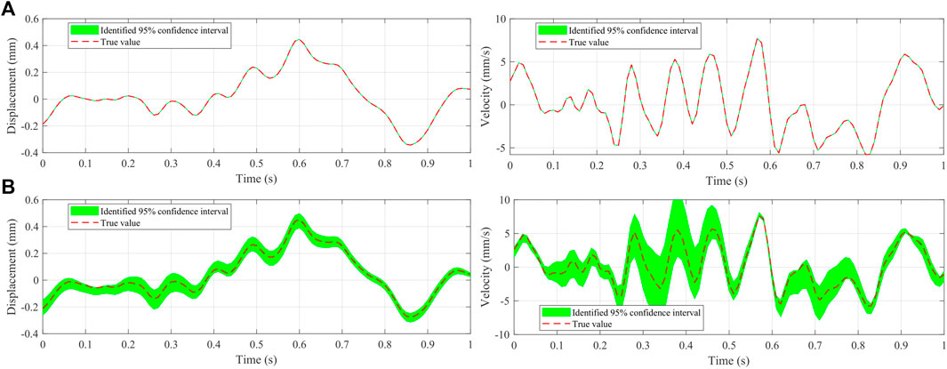
FIGURE 5. Identified displacement and velocity fragments under partial observations. (A) Displacement and velocity responses on the fifth floor. (B) Displacement and velocity responses on the sixth floor. The red dotted line denotes the true trajectory. The green area represents the identified 95% confidence interval.

In the above implementation of the manifold-constrained GPs, all batches were set to contain 50 signal points in order to avoid the impact of batch size on the uncertainty quantification results. Our simulation studies using the manifold-constrained GPs show that the uncertainty can be further lowered when the batch size gets bigger, that is, when more signal points are contained in each batch. However, the enlargement of batch size could lead to computational inefficiency because more variables (the new signal points) are involved and their uncertainties need to be evaluated in each single Hamiltonian Monte Carlo sampling process. Therefore, for practical engineering applications using the manifold-constrained GPs, there is a trade-off between the reduction of uncertainties and the enhancement of computational efficiency. To gain an insight into how exactly the batch size affects the uncertainties of the estimated structural parameters and responses, we compare six different batch sizes containing 20, 30, 40, 50, 60, and 70 signal points, respectively. For each batch size, 20 fragments (with 5% noise corruption) are generated and evaluated by the manifold-constrained GPs. The variances of the stiffness parameter $k_3$ and Rayleigh coefficients $a$ are recorded. Figure 6 shows the boxplots of the recorded data, which indicates that increasing the batch size makes a reduction in the evaluated uncertainties, but overall, the effect is flattening. Moreover, the Rayleigh coefficient is more sensitive to the increment of batch size than the stiffness parameter.

FIGURE 6

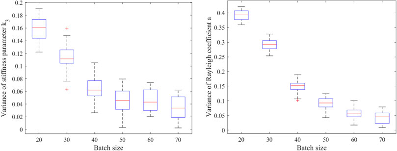
FIGURE 6. Boxplot of variances of stiffness parameter $k_3$ and Rayleigh coefficient $a$.

4 Conclusion

In this study, a manifold-constrained GP approach is explored to estimate the joint posterior probability distributions of the unknown parameters and system state of multi-DOF structures subjected to ground motion. The formulation of the manifold-constrained GPs is intrinsically based on compelling the derivatives of GPs to satisfy the equation of motion of the structural dynamical system. In this approach, the posterior distribution of the unknown parameters and system state is decomposed to be the function of several multivariate Gaussian distributions and the prior distribution of the parameters, in such a way that the high-dimensional integral is avoided in computing joint posterior distributions of the unknown parameters and system state. Thus, the manifold-constrained GPs could provide accurate and computationally efficient inference for multi-DOF systems as addressed in this study. In the case study, the posterior distributions of the system state and unknown parameters are successfully identified in both full observation and partial observation scenarios, from which model updating and damage identification could be further pursued.

Data Availability Statement

The original contributions presented in the study are included in the article/Supplementary Material; further inquiries can be directed to the corresponding author.

Author Contributions

SH: Conceptualization, methodology, software, validation, writing—original draft, and visualization. Y-QN: Conceptualization, supervision, funding acquisition, project administration, and writing—review and editing. S-MW: Conceptualization and supervision.

Funding

The research described in this study was supported by a grant from the Research Grants Council of the Hong Kong Special Administrative Region (SAR), China (Grant no. PolyU 152014/18E); a grant from the National Natural Science Foundation of China (Grant no. U1934209); and grants from Wuyi University’s Hong Kong and Macao Joint Research and Development Fund (Grants nos. 2019WGALH15 and 2019WGALH17). The authors would also like to appreciate the funding support by the Innovation and Technology Commission of the Hong Kong SAR Government to the Hong Kong Branch of the Chinese National Rail Transit Electrification and Automation Engineering Technology Research Center (Grant no. K-BBY1).

Conflict of Interest

The authors declare that the research was conducted in the absence of any commercial or financial relationships that could be construed as a potential conflict of interest.

Publisher’s Note

All claims expressed in this article are solely those of the authors and do not necessarily represent those of their affiliated organizations, or those of the publisher, the editors, and the reviewers. Any product that may be evaluated in this article, or claim that may be made by its manufacturer, is not guaranteed or endorsed by the publisher.

References

Adeagbo, M. O., Lam, H.-F., and Ni, Y. Q. (2021). A Bayesian Methodology for Detection of Railway Ballast Damage Using the Modified Ludwik Nonlinear Model. Eng. Struct. 236, 112047. doi:10.1016/j.engstruct.2021.112047

CrossRef Full Text | Google Scholar

Beck, J. L., and Yuen, K.-V. (2004). Model Selection Using Response Measurements: Bayesian Probabilistic Approach. J. Eng. Mech. 130, 192–203. doi:10.1061/(asce)0733-9399(2004)130:2(192)

CrossRef Full Text | Google Scholar

Behmanesh, I., Moaveni, B., Lombaert, G., and Papadimitriou, C. (2015). Hierarchical Bayesian Model Updating for Structural Identification. Mech. Syst. Signal Process. 64-65, 360–376. doi:10.1016/j.ymssp.2015.03.026

CrossRef Full Text | Google Scholar

Behmanesh, I., and Moaveni, B. (2014). Probabilistic Identification of Simulated Damage on the Dowling Hall Footbridge through Bayesian Finite Element Model Updating. Struct. Control Health Monit. 22, 463–483. doi:10.1002/stc.1684

CrossRef Full Text | Google Scholar

Capellari, G., Eftekhar Azam, S., and Mariani, S. (2015). Damage Detection in Flexible Plates through Reduced-Order Modeling and Hybrid Particle-Kalman Filtering. Sensors 16, 2. doi:10.3390/s16010002

PubMed Abstract | CrossRef Full Text | Google Scholar

Catbas, F. N., Kijewski-Correa, T., and Aktan, A. E. (2013). Structural Identification of Constructed Systems. Reston: ASCE Press.

Google Scholar

Chen, J., and Li, J. (2004). Simultaneous Identification of Structural Parameters and Input Time History from Output-Only Measurements. Comput. Mech. 33, 365–374. doi:10.1007/s00466-003-0538-9

CrossRef Full Text | Google Scholar

Erazo, K., and Nagarajaiah, S. (2018). Bayesian Structural Identification of a Hysteretic Negative Stiffness Earthquake Protection System Using Unscented Kalman Filtering. Struct. Control Health Monit. 25, e2203. doi:10.1002/stc.2203

CrossRef Full Text | Google Scholar

Hassiotis, S., and Jeong, G. D. (1995). Identification of Stiffness Reductions Using Natural Frequencies. J. Eng. Mech. 121, 1106–1113. doi:10.1061/(asce)0733-9399(1995)121:10(1106)

CrossRef Full Text | Google Scholar

Huang, Y., Beck, J. L., and Li, H. (2017). Bayesian System Identification Based on Hierarchical Sparse Bayesian Learning and Gibbs Sampling with Application to Structural Damage Assessment. Comput. Methods Appl. Mech. Eng. 318, 382–411. doi:10.1016/j.cma.2017.01.030

CrossRef Full Text | Google Scholar

Kamariotis, A., Chatzi, E., and Straub, D. (2022). Value of Information from Vibration-Based Structural Health Monitoring Extracted via Bayesian Model Updating. Mech. Syst. Signal Process. 166, 108465. doi:10.1016/j.ymssp.2021.108465

CrossRef Full Text | Google Scholar

Lei, Y., Xia, D., Erazo, K., and Nagarajaiah, S. (2019). A Novel Unscented Kalman Filter for Recursive State-Input-System Identification of Nonlinear Systems. Mech. Syst. Signal Process. 127, 120–135. doi:10.1016/j.ymssp.2019.03.013

CrossRef Full Text | Google Scholar

Li, P. J., Xu, D. W., and Zhang, J. (2016). Probability-based Structural Health Monitoring through Markov Chain Monte Carlo Sampling. Int. J. Str. Stab. Dyn. 16, 1550039. doi:10.1142/s021945541550039x

CrossRef Full Text | Google Scholar

Lu, Z. R., and Law, S. S. (2007). Identification of System Parameters and Input Force from Output Only. Mech. Syst. Signal Process. 21, 2099–2111. doi:10.1016/j.ymssp.2006.11.004

CrossRef Full Text | Google Scholar

Morassi, A., and Tonon, S. (2008). Dynamic Testing for Structural Identification of a Bridge. J. Bridge Eng. 13, 573–585. doi:10.1061/(asce)1084-0702(2008)13:6(573)

CrossRef Full Text | Google Scholar

Neal, R. M. (2010). “MCMC Using Hamiltonian Dynamics,” in Handbook of Markov Chain Monte Carlo. Editors S. Brooks, A. Gelman, G. Jones, and X. L. Meng (Boca Raton: CRC Press), 113–162.

Google Scholar

Ni, Y. Q., Zhou, X. T., and Ko, J. M. (2006). Experimental Investigation of Seismic Damage Identification Using PCA-Compressed Frequency Response Functions and Neural Networks. J. Sound Vib. 290, 242–263. doi:10.1016/j.jsv.2005.03.016

CrossRef Full Text | Google Scholar

Raissi, M., Perdikaris, P., and Karniadakis, G. E. (2017). Inferring Solutions of Differential Equations Using Noisy Multi-Fidelity Data. J. Comput. Phys. 335, 736–746. doi:10.1016/j.jcp.2017.01.060

CrossRef Full Text | Google Scholar

Ramancha, M. K., Astroza, R., Conte, J. P., Restrepo, J. I., and Todd, M. D. (2020). Bayesian Nonlinear Finite Element Model Updating of a Full-Scale Bridge-Column Using Sequential Monte Carlo. Model. Validation Uncertain. Quantification 3, 389–397. doi:10.1007/978-3-030-47638-0_43

CrossRef Full Text | Google Scholar

Rasmussen, C. E., and Williams, C. K. I. (2006). Gaussian Processes for Machine Learning. Cambridge: MIT Press.

Google Scholar

Rocchetta, R., Broggi, M., Huchet, Q., and Patelli, E. (2018). On-line Bayesian Model Updating for Structural Health Monitoring. Mech. Syst. Signal Process. 103, 174–195. doi:10.1016/j.ymssp.2017.10.015

CrossRef Full Text | Google Scholar

Sandesh, S., and Shankar, K. (2009). Time Domain Identification of Structural Parameters and Input Time History Using a Substructural Approach. Int. J. Str. Stab. Dyn. 09, 243–265. doi:10.1142/s0219455409003016

CrossRef Full Text | Google Scholar

Shi, Z. Y., Law, S. S., and Zhang, L. M. (2002). Improved Damage Quantification from Elemental Modal Strain Energy Change. J. Eng. Mech. 128, 521–529. doi:10.1061/(asce)0733-9399(2002)128:5(521)

CrossRef Full Text | Google Scholar

Sun, H., and Betti, R. (2015). A Hybrid Optimization Algorithm with Bayesian Inference for Probabilistic Model Updating. Computer-Aided Civ. Infrastructure Eng. 30, 602–619. doi:10.1111/mice.12142

CrossRef Full Text | Google Scholar

Sun, H., and Betti, R. (2013). Simultaneous Identification of Structural Parameters and Dynamic Input with Incomplete Output-Only Measurements. Struct. Control Health Monit. 21, 868–889. doi:10.1002/stc.1619

CrossRef Full Text | Google Scholar

Wan, H.-P., and Ni, Y.-Q. (2018). Bayesian Modeling Approach for Forecast of Structural Stress Response Using Structural Health Monitoring Data. J. Struct. Eng. 144, 04018130. doi:10.1061/(asce)st.1943-541x.0002085

CrossRef Full Text | Google Scholar

Wan, H.-P., and Ni, Y.-Q. (2019). Bayesian Multi-Task Learning Methodology for Reconstruction of Structural Health Monitoring Data. Struct. Health Monit. 18, 1282–1309. doi:10.1177/1475921718794953

CrossRef Full Text | Google Scholar

Xue, Y., Liu, Y., Ji, C., Xue, G., and Huang, S. (2020). System Identification of Ship Dynamic Model Based on Gaussian Process Regression with Input Noise. Ocean. Eng. 216, 107862. doi:10.1016/j.oceaneng.2020.107862

CrossRef Full Text | Google Scholar

Yang, S., Wong, S. W. K., and Kou, S. C. (2021). Inference of Dynamic Systems from Noisy and Sparse Data via Manifold-Constrained Gaussian Processes. Proc. Natl. Acad. Sci. U.S.A. 118, e2020397118. doi:10.1073/pnas.2020397118

PubMed Abstract | CrossRef Full Text | Google Scholar

Zhou, K., and Tang, J. (2018). Uncertainty Quantification in Structural Dynamic Analysis Using Two-Level Gaussian Processes and Bayesian Inference. J. Sound Vib. 412, 95–115. doi:10.1016/j.jsv.2017.09.034

CrossRef Full Text | Google Scholar

Zhou, K., and Tang, J. (2021a). Structural Model Updating Using Adaptive Multi-Response Gaussian Process Meta-Modeling. Mech. Syst. Signal Process. 147, 107121. doi:10.1016/j.ymssp.2020.107121

CrossRef Full Text | Google Scholar

Zhou, K., and Tang, J. (2021b). Uncertainty Quantification of Mode Shape Variation Utilizing Multi-Level Multi-Response Gaussian Process. J. Vib. Acoust. 143, 011003. doi:10.1115/1.4047700

CrossRef Full Text | Google Scholar