 Wang Junqi
 Wang Ziyan
 Wei Xiaoting
95% of researchers rate our articles as excellent or good
Learn more about the work of our research integrity team to safeguard the quality of each article we publish.
Find out more
ORIGINAL RESEARCH article
Front. Built Environ. , 25 August 2022
Sec. Geotechnical Engineering
Volume 8 - 2022 | https://doi.org/10.3389/fbuil.2022.927100
This article is part of the Research Topic Insights in Geotechnical Engineering: 2021 View all 6 articles
Based on the measured fracture production of the rock body in the field, the disc fracture hypothesis is used to generate three groups of fractures to form a fracture network by the Monte-Carlo method. The three-dimensional fracture network is simplified into a spatial one-dimensional pipe element model based on the hypothesis of water channel flow in the fractures, and the equivalent pipe diameter of the pipe element is considered to be linearly related to the fracture width. The equivalent permeability tensor is obtained by using a genetic algorithm to obtain the ratio of the equivalent pipe diameter to aperture size for each group of fissures, and compared with the equivalent permeability tensor obtained by the overall single-parameter model and direct algorithm. In comparison with the measured permeability tensor, it is concluded that the multiparameter model can better characterize the permeability tensor than the single-parameter model.
Seepage is the flow of fluids in pore media, and the analysis of seepage in fractured rock is very important for human production and life, such as oil storage and underground storage of nuclear waste (Javadi et al., 2010). Therefore, the problem of seepage in fractured rock has been widely concerned and studied. It was found that rock mass discontinuity is discontinuous and extremely irregularly developed, and the fracture network is very complex. To facilitate the study, many scholars have used computer technology to generate discrete fracture network models to carry out research on the permeability characteristics of the simulation models (Witherspoon and Long, 1987; Song and Xu, 2004; Wang et al., 2016). These studies have widely used the permeability tensor to characterize the fracture permeability properties. The nature of the tensor allows the transformation of a discontinuous fractured rock into a continuous medium model for solving the seepage field (Ansari et al., 2016), simplifying calculations and making the solution of large-scale engineering problems possible.
Currently, the two main methods used to study the permeability tensor are the experiment and numerical analysis methods. For the former method, based on the principle of oscillatory micro-water testing, the permeability coefficient tensor of the rock mass was determined in situ by a single-borehole slug test (Zhou et al., 2015). The permeability test was carried out on gabbro shear fractures taken from the Danjiangkou reservoir area under different surrounding pressure and fracture water pressure, based on which the permeability coefficient was corrected considering the changes in three-dimensional stress and fracture water pressure to obtain a new expression for the permeability tensor (Yang et al., 2013). The fracture structure surface parameters were obtained through field measurements and used the discrete element method for seepage analysis (Li and Zhang, 2016). In terms of numerical analysis, the discrete fracture model was applied to study the characteristics of the permeability tensor for different rock discontinuity systems by a planar seepage analysis method (Wang et al., 2013). Based on the UDEC (Universal Distinct Element Code) computing platform, the discrete fracture network model was used to investigate the permeability tensor and analyzed the anisotropy of the permeability tensor (Baghbanan and Jing, 2007). From the literature, it can be found that the numerical method is mainly an analytical calculation of fracture seepage in the case of a two-dimensional model, which differs considerably from the actual situation. In terms of research on 3D models, the boundary element method is used to calculate the permeability tensor of a 3D fracture network, and the permeability tensor is used to quantify the fracture seepage flow (Li and Chen, 2006). The fracture network is generated based on the geometric distribution nature of the fracture, and the triangular element network is divided on the fractured disk to simulate the complex flow and the transport of CO2 in the fracture by numerical methods (Lee and Ni, 2015). Cacas et al. (1990) considered that the seepage in the fissure is channeling, so they proposed to simplify the 3D fracture network into one-dimensional pipe elements, which provided a new idea for the analysis and calculation of seepage flow (Cacas et al., 1990). Wang et al.’s (2002) hydraulic pressure test is used to correct the results of the pipe element model, and the permeability tensor is obtained using the regression analysis. Yu et al. (2006) established a discontinuous fracture network pipe element seepage model and calibrated the model. Wang et al. (2015) used a single-parameter model to determine the element pipe diameter by the inversion method and calculated the permeability tensor of the fractured rock mass using the finite element method.
Some of the above literature studies on seepage calculations focus on the analysis of planar networks, which do not reflect spatial effects; however, there are analytical spatial networks with planar triangular elements, with a large computational scale. Some studies of spatial networks use the one-dimensional pipe element model, but the application of the pipe element model lacks verification of engineering data, and the diameter of the pipe element is determined only by limited piezometric tests, which is difficult to reflect the effects of spatial networks; in addition, due to the geostress history effect, the spatial joints subjected to multi-period tectonic movement and the grouping joints effect appeared, so this article proposes a multiparameter model to reflect the spatial clustering effect of the joints.
The pipe element model is similar to the flow pattern of water between the fissures, which effectively reduces the computational effort, so this article will also use the pipe element model for seepage analysis. The difference is that in the previous pipe element model, there is only one parameter as the ratio of equivalent pipe diameter and aperture size; in this article, multiple groups of fracture networks will be generated in the three-dimensional fracture network model, and each group of fractures will be labeled with the ratio of pipe diameter and aperture size as the corresponding parameters, and the permeability tensor determined by the finite element method will be studied by the multiparameter model.
In engineering practice, the rock discontinuity system may appear to be random, but the aggregation of their characteristic data reveals that the distribution conforms to certain distribution patterns. The statistical model of the characteristic data of the rock structure surface is established by sampling field measurements and then statistical analysis, and computer technology is used to generate a fracture network model with statistical characteristics that match the field measurements (Zhang et al., 2004).
Over years, there are various fracture network models used to characterize the rock discontinuity system. Among those models, the Baecher model is widely used due to its simplicity and practicality (Wang et al., 2010). In this article, we assume that the fractures in the rock mass are discs. The distribution of fracture geometry parameters is determined through field investigations, and then the Monte-Carlo method is used to generate a fracture network, and the useless fractures are excluded. In the process of generation, each fracture in each group is numbered separately.
For the convenience of application, a three-dimensional spatial coordinate system is established, with the XOY plane horizontal and the Z-axis straight up. In using the dip angle dip to find the plane equation, we need to know the direction of the X-axis; here, it refers to the geological compass direction; that is, the north direction is 0°, the east direction is 90°, and the south direction is 180°. The X-axis is defined as pointing east, the Y-axis is north, and the Z-axis is plumb up.
As shown in Figure 1, the unit normal vector of a rift is used to represent its direction. Suppose the unit normal vector of a rift is OP, point N is the vertical projection of point P on the XOY plane, θ is the angle between OP and Z-axis clockwise, and ϕ is the angle between X-axis and ON anti-clockwise. The unit normal vectors of this fissure are l, m, and n, and their values are
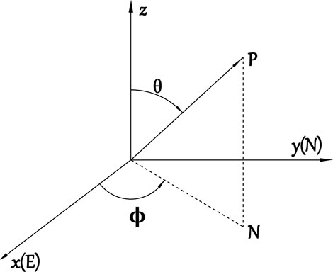
FIGURE 1. Fracture vector coordinates.
In geology, the direction of the fissure is expressed by dip direction α and dip β. If the coordinate system points east by the X-axis and north by the vertical axis, the relationship between (θ, ϕ) and (α, β) can be calculated by the following equation:
Planar seepage assumes that the fractures are discs of thickness and that water flows over the entire fracture disc. The number of fractures is large and the workload of finite element calculation is very heavy, which causes a lot of inconvenience to the research work. In this article, the seepage path of water in a fracture is simplified to a pipe element model based on the previous assumption of trench flow. In other words, the center of the intersecting fractures and the center of the intersection line are used as the nodes of the pipe element, and two adjacent nodes form a pipe element so that the flow of water between the fractures is simplified to the flow between the channels of the pipe element. According to the group number of the fracture plane where the pipe element is located, the pipe element is then classified, as shown in Figure 2.

FIGURE 2. Pipe element of the fracture network.
Assuming that the flow path of the pipe element is circular, the flow rate through the flow path is (Zhang and Sanderson, 2002)
where ΔH is the difference in the head between two nodes; L is the distance between the two nodes; D is the pipe element diameter;
According to Eq. 1, the flow rate through two nodes (i and j) in any pipe element m can be obtained as follows:
where nodal flow q is positive for inflows and negative for outflows. In matrix terms, this can be expressed in the following form:
The above equation can be simplified to
where K is called the total permeability matrix. It is obtained by iterating over all the element permeability matrices
From Eq. 1, it is necessary to know the size of diameter D of each pipe element for the seepage calculation. According to the proportional relationship between the equivalent pipe diameter and the aperture size of the fracture, the ratio of the equivalent pipe diameter to the aperture size of Group i of fractures is set to
Based on the improved genetic algorithm, ratio
Since a change in Ni can affect the magnitude of the principal value of the permeability tensor, the objective function can be expressed as follows:
where
The permeability of the jointed rock mass is expressed using the permeability tensor and has a significant anisotropy, which means that the permeability coefficient varies significantly in each direction. According to the literature (Zhang, 2002), flow rates
where Q is the vector flow, k is the permeability tensor, I is the hydraulic gradient, and A is the overland flow area.
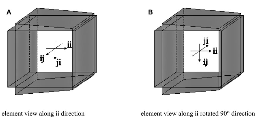
FIGURE 3. Boundary conditions of a computational model.
let q = Q/A be the flow rate per unit area of overflow, Darcy’s law can be written as follows:
For any three-dimensional orthogonal hydraulic slope drop (
Then the permeability tensor is
where
The relative error of the main value of permeability is
where
Since the error of the main direction of permeability cannot be directly derived, the angle between the direction of the main value of the calculated permeability and the direction of the main value of the field pressure water test is the absolute error of the main direction. The cosine of the angle between the two permeability main value directions is
where
The information on the geometric parameters of the fractures was obtained from the literature (Li and Chen, 2006) by actual measurements as shown in Table 1, and three groups of fractures were measured.
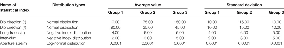
TABLE 1. Statistical parameters of the fracture network.
The literature (Li and Chen, 2006) used the boundary element method to calculate the permeability tensor of the fracture network in Table 1, and the main value of permeability and the main direction were obtained by the field piezometric test for calibration as in Eq. 7, which was used as the target permeability tensor for the later pipe diameter inversion:
A self-programmed fracture network finite element program was used to simulate the fracture network by inputting the information in Table 1 into the program.
The authors use a C++ compiler to write a 3D fracture network finite element program in a multiparameter model state, and the main functions of the program are as follows: 1) Generate the fracture network according to the geometric distribution law of the fracture structure surface, and eliminate the fractures that are useless for hydraulic conductivity by a path search, which simplifies the calculation. 2) The fracture disc is simplified into a pipe unit model, and in the process of simplification, the fractures where the equivalent pipe units are located are discriminated, the groups where the fractures are located are identified, and the pipe units in the same group are categorized. In the inversion, different parameters are set as ratios according to the category of pipe units. 3) Using the improved genetic algorithm, the optimal values of the parameters are determined by fitting the multiparameter calculation at the same time. 4) The main value and main direction of permeability of the 3D fractured rock mass under the multiparameter model are obtained by calculation. Figure 4 is the flow chart of the program.
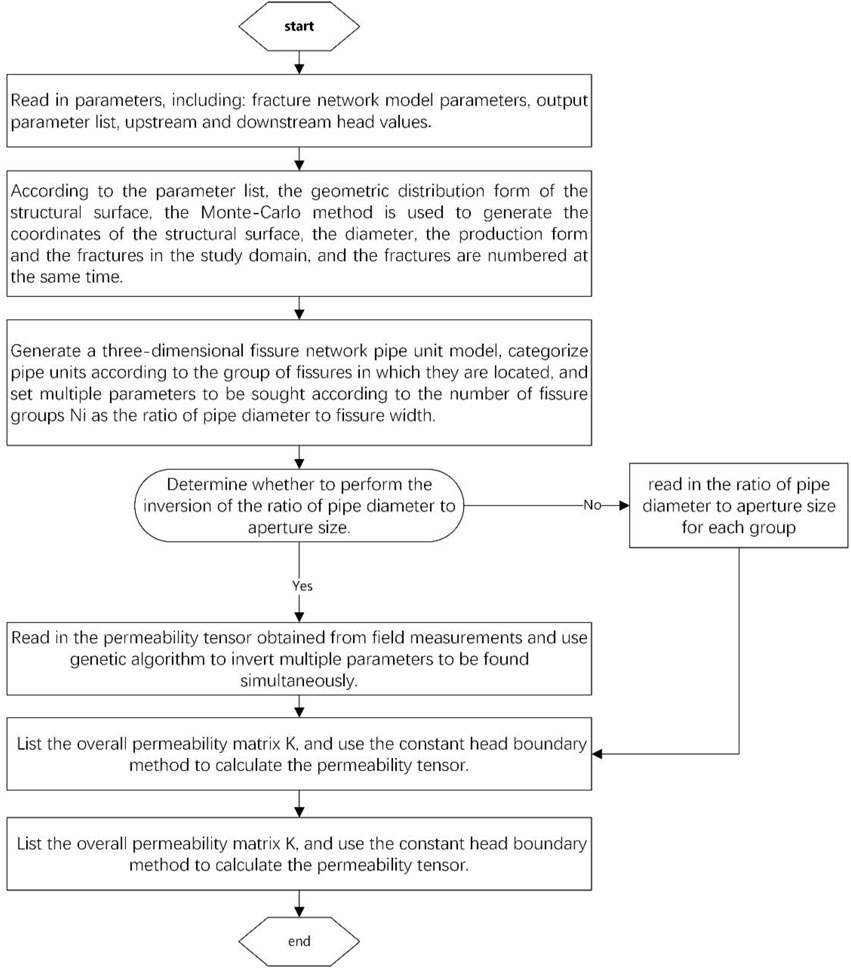
FIGURE 4. Calculation flowchart.
The generated domain of the program is a cubic area of 100 m × 100 m × 100 m, in which a cubic area of 20 m × 20 m × 20 m is intercepted as the study domain. The Monte-Carlo method is used to generate a three-dimensional fracture network. A total of 2,00,255 structural surfaces are generated in the generated domain, including 1,29,006 structural surfaces in Group 1, 38,224 structural surfaces in Group 2, and 33,025 structural surfaces in Group 3. In the study domain, a total of 911 structural surfaces are generated after excluding the fractures that do not contribute to seepage, including 480 structural surfaces in Group 1, 250 structural surfaces in Group 2, and 181 structural surfaces in Group 3. Simplifying them into a pipe element model, 4104 elements are obtained with 3033 nodes, and the generated fracture network is shown in Figure 5.
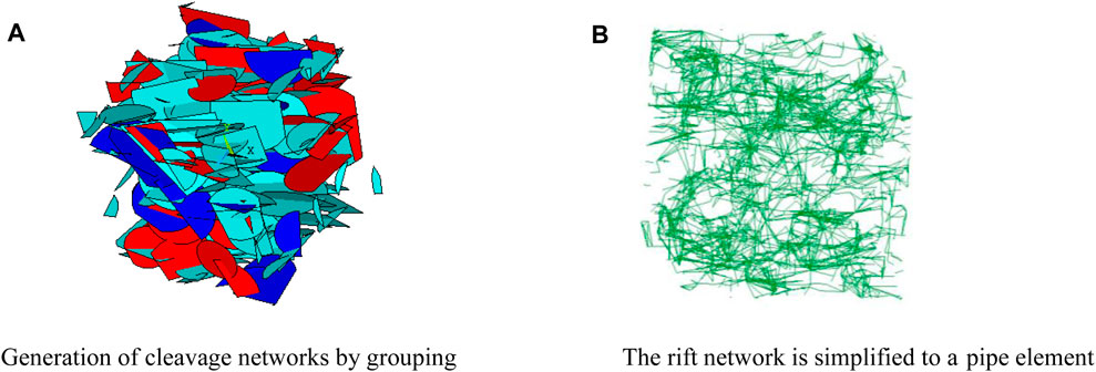
FIGURE 5. Three-dimensional fracture network. (A) Element view along ii direction. (B) Element view along ii rotated 90° direction.
During the numerical calculation, the head boundary was set at
Using Eq. 7 as a criterion for the fit, the three parameters were obtained by optimal fitting equal to 13.17, 12.06, and 3.01, respectively.
The head distribution of the multiparameter model is calculated as shown in Figure 6, with the following permeability tensor (in m/s):
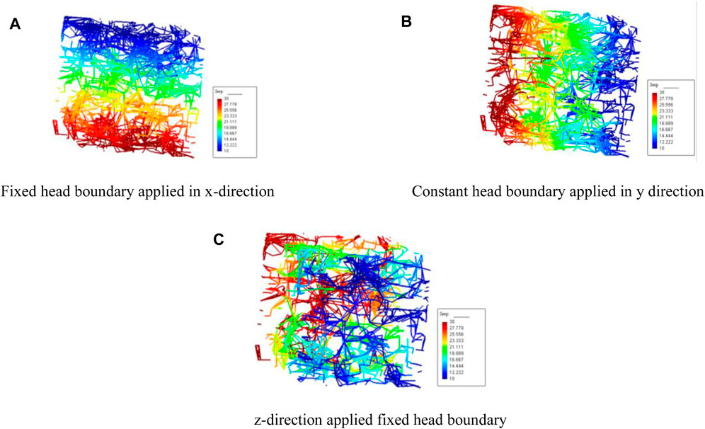
FIGURE 6. Three groups of simulated head distribution: (A) fixed head boundary applied in the x-direction, (B) constant head boundary applied in y-direction, and (C) z-direction applied fixed head boundary.
Since the permeability tensor belongs to the second-order tensor, the eigenvalues of permeability tensor matrix k are the permeability principal values, and its eigendirection is the permeability principal direction. The principal values of permeability and the principal directions of permeability obtained from the permeability tensor are as follows:
Compared with the data in Eq. 7, the error is
where ε is the relative error of the main value and θ is the absolute error of the main direction.
The single-parameter model approach of the literature was used to numerically simulate the three-dimensional fracture network seepage model (Wang et al., 2015).
Parameter N is set as the ratio of the equivalent pipe diameter to the aperture size for the three sets of fractures in the calculation process.
With the information shown in Table 1, the value of parameter N is obtained as 12.34 and the result of its permeability tensor (in m/s) is as follows:
The main coefficient of permeability and the main direction of permeability are as follows:
Compared with the data of Eq. 7, the error is
where ε is the relative error of the main value and θ is the absolute error of the main direction.
The relative error in the main value of penetration is larger for the single-parameter model than for the multiparameter model.
The distribution of aperture sizes in the above two sections obeys a log-normal distribution with a mean of 0.0001 and a standard deviation of 0.0001. In this section, all aperture sizes of the cleft are set to a constant value of 0.0001, and other geometric parameters remain unchanged.
The values of the parameters of the multiparameter model for the case of the study domain size of 20 m × 20 m × 20 m are 19.51,16.55, and 14.05, and the permeability tensor (in m/s) is
The one-parameter model has a parameter value of 16.46 and a permeability tensor of
The mean values of the parameters obtained for the multiparameter model by varying the size of the study domain with those of the single-parameter model are shown in Table 2.
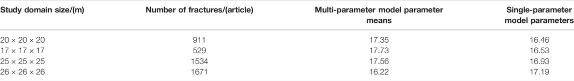
TABLE 2. The parameter values of the model.
From the calculation results of Eq. 16 and Eq. 19, it can be seen that the errors in the main value of permeability and the main direction of permeability for both models are within the engineering allowable range for a fixed aperture size.
After determining the seepage area based on the literature, the area of the seepage basin is calculated by integration (Wang et al., 2002), and then the area of the area is replaced by a regular rectangle. In this article, the seepage area is simplified to a pipe element to find its pipe diameter, where Eqs 21–25 include the derivation process. Figure 7 illustrates the simplified process.
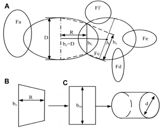
FIGURE 7. Simplified diagram of pipe element.
By Darcy’s law,
According to the geometric relationship in the figure, Eq. 20 can be written as follows:
where Q is the given seepage flow rate, K is the permeability coefficient,
The integral formula leads to
Then the diameter of the pipe element can be written as follows:
The area of the irregular seepage region is calculated by the integral method, the area is replaced by a regular rectangle equivalent, and the fractured disk is simplified to a pipe element to simulate the seepage between the intersecting fractures and perform the calculation of the fracture permeability tensor. According to Sections 2.3, 3.2, the calculation of the permeability tensor is as follows:
The main coefficient of permeability and the main direction of permeability are as follows:
Compared with the data of Eq. 7, the error is as follows:
It is found that the absolute error of the principal value of the direct algorithm is smaller than that of the single-parameter and larger than that of the multiparameter model; the errors in the main direction of penetration are larger than those of the single-parameter and multiparameter models.
The calculation results in Sections 4.2, 4.3, and 4.5 show that when the aperture size obeys log-normal distribution, the sum of absolute errors in the main direction is 63.04 for the multiparameter model, 63.1 for the single-parameter model, and 101.4 for the direct algorithm. The errors of the multiparameter and single-parameter models are consistent, and the errors of the direct method are larger. In terms of the error principal component of the seepage tensor, the error of the multiparameter model is significantly smaller than that of the single-parameter model with the direct algorithm. From the calculation results, the multiparameter model is significantly optimized in the main direction of the permeability tensor as well as the main value, which is more in line with the actual situation. The reason for this is that in the process of optimization, under the condition that the objective function Eq. 4 meets the requirements, the corresponding principal direction and the principal direction of the target tensor remain basically the same; that is, the angle between the two is an acute angle.
When the aperture size of the fracture network is constant, the single-parameter model gives better results than the multiparameter model. This is because when the aperture size is constant, the ratio of the pipe diameter to the aperture size of each element is close to the same number, so the single parameter model gives more accurate results. It is also found from Table 2 that the mean parameter values of the multiparameter model for a constant aperture size are approximately equal to those of the single-parameter model, and fluctuate around 17.00 for different research domain sizes.
1) In this article, a three-dimensional discrete fracture network model is used to simplify the complex fractured rock into a pipe element model, and multiple parameters are set in the numerical analysis to obtain the permeability tensor. From the calculation results of project measured data, it can be seen that when the aperture size obeys log-normal distribution, the error of the multiparameter model is smaller, and it is suitable to choose the multiparameter model in this case. When the mean aperture size is a constant size, a single-parameter model is suitable for the calculation and analysis.
2) From the calculation results of Eq. 10, we can find that the calculated results of the multiparameter model have relatively small errors in both the main value of permeability and the main direction of permeability. This indicates that in engineering applications, the use of multiparameter models for simulation can improve the accuracy of permeability analysis and has better theoretical and practical properties.
The raw data supporting the conclusions of this article will be made available by the authors, without undue reservation.
WJ: conceptualization, methodology, software, investigation, formal analysis, and writing—original draft. WZ: software, validation, data organization, and writing—original draft. WX: visualization, investigation, and supervision.
The authors declare that the research was conducted in the absence of any commercial or financial relationships that could be construed as a potential conflict of interest.
All claims expressed in this article are solely those of the authors and do not necessarily represent those of their affiliated organizations, or those of the publisher, the editors, and the reviewers. Any product that may be evaluated in this article, or claim that may be made by its manufacturer, is not guaranteed or endorsed by the publisher.
Ansari, M. A., Deodhar, A., Kumar, U. S., Davis, D., and Somashekar, R. K. (2016). “Isotope Hydrogeological Factors Control Transport of Radon-222 in Hard Rock Fractured Aquifer of Bangalore, Karnataka,” in Geostatistical and Geospatial Approaches for the Characterization of Natural Re-sources in the Environment (Berlin, Germany: Springer International Publishing), 259–265. doi:10.1007/978-3-319-18663-4_40
Baghbanan, A., and Jing, L. (2007). Hydraulic Properties of Fractured Rock Masses with Correlated Fracture Length and Aperture. Int. J. Rock Mech. Min. Sci. 44 (5), 704–719. doi:10.1016/j.ijrmms.2006.11.001
Cacas, M. C., Ledoux, E., de Marsily, G., Tillie, B., Barbreau, A., Durand, E., et al. (1990). Modeling Fracture Flow with a Stochastic Discrete Fracture Network: Calibration and Validation: 1. The Flow Model. Water Resour. Res. 26 (3), 479–489. doi:10.1029/WR026i003p00479
Javadi, M., Sharifzad, M., and Shahriar, K. (2010). A New Geometrical Model for Non-linear Fluid Flow through Rough Fractures. J. Hydrology 389, 18. doi:10.1016/j.jhydrol.2010.05.010
Lee, I. H., and Ni, C. F. (2015). Fracture-based Modeling of Complex Flow and CO2 Migration in Three-Dimensional Fractured Rocks. Comput. Geosciences 81, 64–77. doi:10.1016/j.cageo.2015.04.012
Li, K., and Zhang, Y. (2016). Analysis of Seepage Characteristics of Rock Mass Based on Measured Structural Plane[J]. Surv. Sci. Technol. 2016 (1), 1.
Li, X., and Chen, Z. (2006). Boundary Element Method and Program for Seepage Calculation of Three-Dimensional Fracture Network[J]. J. China Inst. Water Resour. Hydropower Res. 4 (2), 86.
Song, X., and Xu, W. (2004). A Study on Conceptual Models of Fluid Flow in Fractured Rock[J]. Rock Soil Mech. 25 (2), 226.
Wang, J., Yue, X., and Li, C. (2015). Three-dimensional Pipe Element Model in Fractured Rock Mass for Determining Seepage Tensor[J]. J. North China Electr. Power Univ. 42 (1), 108.
Wang, M., Kulatilake, P. H. S. W., Um, J., and Narvaiz, J. (2002). Estimation of REV Size and Three-Dimensional Hydraulic Conductivity Tensor for a Fractured Rock Mass through a Single Well Packer Test and Discrete Fracture Fluid Flow Modeling. Int. J. Rock Mech. Min. Sci. 39, 887–904. doi:10.1016/s1365-1609(02)00067-9
Wang, P., Yang, T., Yu, Q., Liu, H., Xia, D., and Zhang, P. (2013). Permeability Tensor and Seepage Properties for Jointed Rock Masses Based on Discrete Fracture Network Model[J]. Rock Soil Mech. 34 (2), 448.
Wang, X., Jia, Z., Zhang, F., and Li, X. (2010). Principle of Mesh Simulation of Rock Mass Discontinuity and Its Engineering Application[M]. Beijing: Water Resources and Hydropower Press, 83.
Wang, Z., Zhang, Z., Li, S., Bi, L., Fang, S., and Zhong, K. (2016). Assessment of Inter-cavern Containment Property for Underground Oil Storage Caverns Using Discrete Fracture Networks[J]. J. SHANDONG Univ. Eng. Sci. 46 (2), 94.
Witherspoon, P. A., and Long, J. C. S. (1987). “Some Recent Development in Understanding the Hydrology of Fractured Rocks[C],” in Proceeding of 28th US Symposium on Rock Mechanics, 422.
Yang, J., Lei, L. I., and Ni, X. I. E. (2013). Hydraulic Conductivity Tensor for Fractured Rock Mass Considering Stress State[J]. Yellow River 2013 (3), 133.
Yu, Q., Wu, X., and Yuzo, O. (2006). Channel Model for Fluid Flow in Discrete Fracture Network and its Modification[J]. Chin. J. Rock Mech. Eng. 25 (7), 1469.
Zhang, F., Wang, X., Jia, Z., and Chen, Z. (2004). 3d Joint Persistence Calculation Through Random Simulation[J]. Chin. J. Rock Mech. Eng. 23 (9), 1487.
Zhang, X. (2002). Numerical Modeling and Analysis of Fluid Flow and Deformation of Fractured Rock masses[M]. Oxford, Amsterdam: Elsevier Science Ltd., 53.
Zhang, X., and Sanderson, D. J. (2002). “Numerical Modeling and Analysis of Fluid Flow and Defor— Mation of Fractured Rock Masses[M],” in Evaluation of 2-Dimensional Permeability Tensors (Oxford, Amsterdam: Elsevier Science Ltd), 53–89. doi:10.1016/b978-008043931-0/50016-8
Keywords: multiparameter model, three-dimensional fracture network, pipe element, permeability tensor, seepage tensor
Citation: Junqi W, Ziyan W and Xiaoting W (2022) The Seepage Tensor of the Multiparameter Model of Pipe Element in Fractured Rock Mass. Front. Built Environ. 8:927100. doi: 10.3389/fbuil.2022.927100
Received: 23 April 2022; Accepted: 01 June 2022;
Published: 25 August 2022.
Edited by:
Jie Han, University of Kansas, United StatesCopyright © 2022 Junqi, Ziyan and Xiaoting. This is an open-access article distributed under the terms of the Creative Commons Attribution License (CC BY). The use, distribution or reproduction in other forums is permitted, provided the original author(s) and the copyright owner(s) are credited and that the original publication in this journal is cited, in accordance with accepted academic practice. No use, distribution or reproduction is permitted which does not comply with these terms.
*Correspondence: Wang Junqi, anF3YW5nbWFpbEAxNjMuY29t
Disclaimer: All claims expressed in this article are solely those of the authors and do not necessarily represent those of their affiliated organizations, or those of the publisher, the editors and the reviewers. Any product that may be evaluated in this article or claim that may be made by its manufacturer is not guaranteed or endorsed by the publisher.
Research integrity at Frontiers
Learn more about the work of our research integrity team to safeguard the quality of each article we publish.