Tension Estimation Method for Cable With Damper Using Natural Frequencies and Two-Point Mode Shapes With Uncertain Modal Order

In the maintenance of cable structures, such as cable-stayed bridges, cable safety is assessed based on the cable tension. In Japan, the cable tension is generally estimated from the cable’s natural frequencies using the higher-order vibration method. In recent years, dampers have been installed onto cables to suppress aerodynamic vibrations. Because the damper changes the cable’s natural frequencies, the damper is removed to measure the natural frequencies and estimate the cable tension without a damper, and the damper is then reinstalled. To avoid damper removal and reinstallation, the authors previously proposed Method 2F for estimating the tension of a cable with a damper from the natural frequencies without removing the damper. Because the tension estimation error of the higher-order vibration method for a cable without a damper has been reported as 5%, the authors set the target tension estimation error within 5%. However, the tension estimation error of Method 2F exceeded 5% in the experimental verification. Furthermore, although Method 2F estimates the tension and bending stiffness of the cable and the damper parameters simultaneously from the natural frequencies, the accuracy of the bending stiffness and damper parameters is unsatisfactory. In this paper, the new Method 2FM is proposed to estimate the tension and bending stiffness of the cable and damper parameters using the natural frequencies and two-point mode shapes. With the addition of mode shapes, Method 2FM attempts to improve the accuracy of estimating the tension and other parameters. The validity of Method 2FM was confirmed by numerical simulations and experiments. The numerical verification confirmed that Method 2FM is superior to Method 2F in estimating the cable tension and damper parameters. The experimental verification confirmed that the tension estimation accuracy of Method 2FM is higher than that of Method 2F, and the estimation error is lower than 5%. However, the damper parameters estimated by Method 2FM are different to the design values. The reason for this is the modeling error of the damper, as found by conducting an element test on the damper.

1 Introduction

In Japan, the maintenance policy of cable structures, such as cable-stayed bridges and extra-dosed bridges, prescribes that the tension acting on the cables must be checked every 5 years. The cable tension is mainly estimated from the cable’s natural frequencies based on the vibration method (Shinke et al., 1980; Zui et al., 1996) or higher-order vibration method (Yamagiwa et al., 2000).

The vibration method is based on string theory. However, the actual bridge cable is not a pure string, and the effect of the bending stiffness is not negligible. Therefore, the effect of the bending stiffness is considered using a correlation factor, and the bending stiffness must be determined in advance. However, it is difficult to determine the exact bending stiffness because bridge cables are typically stranded wire.

The higher-order vibration method is based on the tensioned Bernoulli–Euler beam theory. The natural frequency of a cable is expressed as a function of the tension and bending stiffness. Therefore, the higher-order vibration method can estimate the tension and bending stiffness simultaneously from the natural frequencies, and the pre-evaluation of bending stiffness is not required. Therefore, this method is frequently used in current practice.

Various studies have investigated cable tension estimation methods, which include methods dealing with complicated boundary conditions (Chen et al., 2016, 2018; Yan et al., 2019), a method dealing with the uncertain boundary condition of a short cable by introducing an additional mass block (Li et al., 2021), methods dealing with inclined cables (Kim and Park, 2007; Ma, 2017), a method dealing with a cable with flexible supports (Foti et al., 2020), a method dealing with environmental temperature variation (Ma et al., 2021), methods for two cables connected by an intersection clamp (Furukawa et al., 2022a), a method using the power spectrum and cepstrum (Feng et al., 2010), a method using a finite element analysis (Gan et al., 2019), a method using a genetic algorithm and particle swarm optimization (Zarbaf et al., 2017), and a method using neural networks (Zarbaf et al., 2018).

Recently, the aerodynamic vibration of cables has become an issue of interest. Dampers are installed onto cables to suppress cable vibration. Because the damper changes the cable’s natural frequencies, the damper is removed from the cable, the cable’s tension without a damper is estimated using the vibration and higher-order vibration methods, and then the damper is reinstalled. Because the removal and reinstallation of the damper are time-consuming and labor-intensive, a tension estimation method for a cable with a damper is required.

Previous studies on cables with dampers have mostly focused on the optimal design of dampers for suppressing the cable amplitude (Pacheco et al., 1993; Krenk 2000; Tabatabai and Mehrabi, 2000; Izzi et al., 2016; Lazar et al., 2016; Shi and Zhu, 2018; Javanbakht et al., 2019), but have not investigated a tension estimation method.

Studies on a tension estimation method for a cable with a damper are still scarce. Yan et al. (2020) proposed a tension estimation method for cables with two intermediate supports (dampers), and modeled the damper as a spring. The damping force which decays the vibration is ignored, and the damper’s spring constant is assumed to be known. However, because the damper’s performance gradually degrades by aging, it is difficult to obtain the spring constant in advance.

Shan et al. (2019) estimated the tension of a cable with a supplemental damper, and assumed a viscous shear damper with a spring constant and damping coefficient. Their method assumes that the cable’s bending stiffness and damper’s damping coefficient are known a priori. However, as stated above, it is not always possible to accurately obtain the cable’s bending stiffness and damper’s damping coefficient in advance.

Hou et al. (2020) proposed a cable tension estimation method by adding virtual supports using the substructure isolation method. Their method extracts the cable section without a damper by using virtual supports. However, the installation and removal of virtual supports is time-consuming and labor-intensive.

The authors previously proposed three tension estimation methods (Methods 0, 1, and 2F) for a cable with a damper (Furukawa et al., 2021a; Furukawa et al., 2022b). By using the higher-order vibration method, theoretical equations for estimating the tension and bending stiffness of the cable and damper parameters from the natural frequencies of a cable with a damper were derived. The cable’s bending stiffness and the damper parameters do not need to be determined in advance and can be instead estimated simultaneously with the cable tension.

Methods 0F and 1F require the modal order of natural frequencies to be specified, while Method 2F does not. The validity of these three methods was experimentally investigated, and it was observed that some natural frequencies could not be excited because of damping. Therefore, the modal order could not be correctly assigned for the measured natural frequencies, the accuracy of Methods 0F and 1F deteriorated, and Method 2F was found to be the best.

However, Method 2F still has shortcomings. Because the tension estimation error of the higher-order vibration method for a cable without a damper has been reported as 5% (Shinko Wire Company, 2020), the authors set the target tension estimation error within 5%. However, the tension estimation error of Method 2F exceeded 5% in the experimental verification, and the accuracy of parameters other than tension, such as the bending stiffness of the cable and damper parameters, is unsatisfactory.

In the measurement of the natural frequencies of cables with accelerometers, the accelerometers are typically installed onto the cable at more than one points to prevent omissions of natural frequency measurement. Therefore, two-point mode shapes can at least be extracted from the acceleration measurements. This study developed a new estimation method (Method 2FM) for a cable with a damper by using the natural frequencies and two-point mode shapes. Whether the tension estimation accuracy can be improved, whether the bending stiffness and damper parameters can be estimated with reasonable accuracy, and whether a tension estimation error within 5% can be achieved in the experiment, were all questions that this study attempted to answer.

Previous studies have used the mode shapes in addition to the natural frequencies (Chen et al., 2016, 2018; Yan et al., 2019), and introduced mode shapes to deal with the arbitrary boundary conditions of the cable. This approach requires the measurement of mode shapes at multiple locations over the entire length of the cable to avoid the modeling of complicated boundary conditions. However, because it is difficult to install sensors far from the main girder, the proposed method only requires simultaneous measurement at two points near the damper.

The rest of this paper is structured as follows. Section 2 describes the previously proposed Method 2F using the natural frequencies. Section 3 presents the new Method 2FM using the natural frequencies and two-point mode shapes. In Section 4, the numerical verification of 90 numerical models is presented. The natural frequencies and mode shapes of a cable with a damper were calculated for 90 models and input into the new and previously proposed methods. The estimated results were compared to the assumed true values and their accuracy and validity are discussed. Section 5 presents the experimental verification of the proposed method, and the validity of the proposed method is discussed.

2 Previously Proposed Method for Estimating Tension of Cable With Damper Using Natural Frequencies (Method 2F)

2.1 Natural Frequencies of Cable With Damper

In the authors’ previous study, a theoretical formula for estimating the complex natural frequencies of a cable with a damper was derived (Furukawa et al., 2021a). This section explains the derivation of the theoretical formula. Figure 1 shows the analytical model of a cable with a damper and simple supports at the two ends. The cable length is $L$, and the distance from the damper position to the left and right ends is $L_1$ and $L_2(=L-L_1)$, respectively.

FIGURE 1

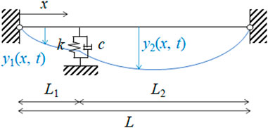
FIGURE 1. Model of cable with damper.

The cable is considered as a tensioned Bernoulli–Euler beam. The vibration equation for a tensioned Bernoulli–Euler beam can be written as the following partial differential equation:

$\rho A\frac{{\partial }^2{y}_d\left(x,t\right)}{\partial t^2}+EI\frac{{\partial }^4{y}_d\left(x,t\right)}{\partial x^4}-T\frac{{\partial }^2{y}_d\left(x,t\right)}{\partial x^2}=0d=1,2(1)$

where $y_d(x,t)$ is the deflection of the cable on the left side $(d=1)$ and right side $(d=2)$ with regard to the damper position, which is a function of position $x$ and time $t$; $\rho$ is the density; $A$ is the cross-sectional area; $EI$ is the bending stiffness; $T$ is the tension.

The deflection of the cable is denoted as $y_1\left(x,t\right)=Y_1\left(x\right)\text{exp}\left(j\omega t\right)$ and $y_2\left(x,t\right)=Y_2\left(x\right)\text{exp}\left(j\omega t\right)$, respectively, using the variable separation method; $Y_1\left(x\right)$ and $Y_2\left(x\right)$ are the modal functions of position $x$; $j$ is an imaginary unit; $\omega$ is the circular frequency. The general solutions of $Y_1\left(x\right)$ and $Y_2\left(x\right)$ are expressed as follows:

$Y_1\left(x\right)=D_1\text{cos}\alpha x+D_2\text{sin}\alpha x+D_3\text{cosh}\beta x+D_4\text{sinh}\beta x (0\le x\le L_1)(2)$

$Y_2\left(x\right)=D_5\text{cos}\alpha \left(x-L_1\right)+D_6\text{sin}\alpha \left(x-L_1\right)+D_7\text{cosh}\beta \left(x-L_1\right)+D_8\text{sinh}\beta \left(x-L_1\right)(L_1\le x\le L)(3)$

where $D_1$, $D_2$, $D_3$, $D_4$, $D_5$, $D_6$, $D_7$, and $D_8$ are the integration constants, and $\alpha$ and $\beta$ are expressed by Eqs 4, 5, respectively.

$\alpha =\sqrt{\sqrt{{\left(\frac{T}{2EI}\right)}^2+\frac{\rho A{\omega }^2}{EI}}-\frac{T}{2EI}}(4)$

$\beta =\sqrt{\sqrt{{\left(\frac{T}{2EI}\right)}^2+\frac{\rho A{\omega }^2}{EI}}+\frac{T}{2EI}}(5)$

Because there are eight integration constants, eight boundary conditions are required. Four boundary conditions are established at the two ends with the simple supports ($Y_1\left(0\right)=0$, $d^2{Y}_1\left(0\right)/d{x}^2=0$, $Y_2\left(L\right)=0$, $d^2{Y}_2\left(L\right)/d{x}^2=0$). Since one continuous cable receives force from the damper only in the direction perpendicular to the cable axis, it is considered that the deflection, deflection angle, and curvature (bending moment) are continuous at the damper position. Therefore, three boundary conditions (continuity equations) are established at the damper position ($Y_1\left(L_1\right)=Y_2\left(L_1\right)$, $d{Y}_1\left(L_1\right)/dx=d{Y}_2\left(L_1\right)/dx$, $d^2{Y}_1\left(L_1\right)/d{x}^2=d^2{Y}_2\left(L_1\right)/d{x}^2$). Moreover, the force exerted on the cable by the damper is equal to the shear force change of the cable at the damper position ($EI{d}^3{Y}_1\left(L_1\right)/d{x}^3-EI{d}^3{Y}_2\left(L_1\right)/d{x}^3=k^{\ast }{Y}_1\left(L_1\right))$; $k^{\ast }$ is the complex stiffness of the damper. The unified notation $k^{\ast }$ is used to model various dampers, as will be explained later.

By substituting Eqs 2, 3 into the eight boundary conditions, the following equation is obtained:

$\text{sin}\alpha L\left\{{\alpha }^2+{\beta }^2+\frac{k^{\ast }}{EI}\left(\frac{\text{sin}\alpha L_1\text{cos}\alpha L_1}{\alpha }-\frac{\text{sinh}\beta L_1\text{sinh}\beta L_2}{\beta \text{sinh}\beta L}\right)\right\}-\text{cos}\alpha L\left(\frac{k^{\ast }}{EI}\frac{{\text{sin}}^2\alpha L_1}{\alpha }\right)=\text{sin}\left(\alpha L-\theta \right)=0(6)$

where

$\text{tan}\theta =\frac{\frac{k^{\ast }}{EI}\frac{{\text{sin}}^2\alpha L_1}{\alpha }}{{\alpha }^2+{\beta }^2+\frac{k^{\ast }}{EI}\left(\frac{\text{sin}\alpha L_1\text{cos}\alpha L_1}{\alpha }-\frac{\text{sinh}\beta L_1\text{sinh}\beta L_2}{\beta \text{sinh}\beta L}\right)}(7)$

Equation 6 has infinite solutions for $\alpha$. These solutions are expressed with a positive integer $i$.

${\alpha }_{i}L-{\theta }_i=i\pi i=\mathrm{1,2},\dots .(8)$

By substituting Eq. 4 into Eq. 8, the natural circular frequency ${\omega }_i$ of the $i$^th mode can be obtained as follows:

${\omega }_i^2=\frac{{\pi }^{4}EI}{\rho A{L}^4}{\left(i+\frac{{\theta }_i}{\pi }\right)}^4+\frac{{\pi }^{2}T}{\rho A{L}^2}{\left(i+\frac{{\theta }_i}{\pi }\right)}^2 i=\mathrm{1,2},\dots (9)$

Finally, the theoretical equation for estimating the natural frequencies $f_i^t$ of the $i$^th mode, and the relevant equations, are expressed as follows:

$f_i^t=\sqrt{\frac{{\pi }^{2}EI}{4\rho A{L}^4}{\left(i+\frac{{\theta }_i}{\pi }\right)}^4+\frac{T}{4\rho A{L}^2}{\left(i+\frac{{\theta }_i}{\pi }\right)}^2} i=\mathrm{1,2},\dots (10)$

${\theta }_i={\text{tan}}^{-1}\frac{\frac{k_i^{\ast }}{EI}\frac{{\text{sin}}^2{\alpha }_i{L}_1}{{\alpha }_i}}{{\alpha }_i^2+{\beta }_i^2+\frac{k_i^{\ast }}{EI}\left(\frac{\text{sin}{\alpha }_i{L}_1\text{cos}{\alpha }_i{L}_1}{{\alpha }_i}-\frac{\text{sinh}{\beta }_i{L}_1\text{sinh}{\beta }_i{L}_2}{{\beta }_i\text{sinh}{\beta }_{i}L}\right)}(11)$

${\alpha }_i=\sqrt{\sqrt{{\left(\frac{T}{2EI}\right)}^2+\frac{\rho A{\left(2\pi f_i^t\right)}^2}{EI}}-\frac{T}{2EI}}(12)$

${\beta }_i=\sqrt{\sqrt{{\left(\frac{T}{2EI}\right)}^2+\frac{\rho A{\left(2\pi f_i^t\right)}^2}{EI}}+\frac{T}{2EI}}(13)$

$k_i^{\ast }=\{\begin{array}{cc}{k}_u+j{k}_v& (\text{high}-\text{damping rubber damper})\\ k+j\left(2\pi f_i^t\right)c& \left(\text{viscous shear damper}\right)\end{array}(14)$

In the case of the high-damping rubber damper, the complex stiffness $k^{\ast }$ is expressed with $k_u$ and $k_v$, which are the real and imaginary parts of the complex stiffness, respectively. In the case of the viscous shear damper, the complex stiffness $k^{\ast }$ is expressed with a spring constant $k$ and damping coefficient $c$.

From the cable parameters, namely, $\rho$, $A$, $L$, $EI$, and $T$, and the damper parameters $k_u$ and $k_v$ or $k$ and $c$, the $i$^th mode natural frequencies $f_i^t$ can be calculated using Eqs 10–13, Eq. 14. Because the natural frequency $f_i^t$ of the $i$^th mode is included on the right-hand side of Eqs 12, 13, Eq. 14b. Eqs 10–13, Eq. 14 must be satisfied simultaneously. Notably, $f_i^t$ in Eq. 10 is a complex value if $k^{\ast }$ is complex. Therefore, this study refers to $f_i^t$ as the complex natural frequency.

The real part of the complex natural frequency $\text{Re}\left(f_i^t\right)$ represents the natural frequency of a cable with a damper and can be obtained by measurement.

The imaginary part of the frequency $\text{Im}\left(f_i^t\right)$ is related to the damping factor or logarithmic decrement. Because the damping factor$$ is difficult to measure with high accuracy, this study considered that only the real parts of the complex natural frequencies of several modes can be measured and used in the estimation.

2.2 Method 2F

The $i$^th mode complex natural frequency $f_i^t$ can be written using $H_i$, as follows:

$f_i^t=Re\left(f_i^t\right)\left(1+j\frac{Im\left(f_i^t\right)}{Re\left(f_i^t\right)}\right)=Re\left(f_i^t\right)\left(1+j{H}_i\right)(15)$

where $H_i$ is defined as the ratio of the imaginary part to the real part of the complex natural frequency and is related to the damping factor $h_i$ of the $i$^th mode ($H_i=h_i/\sqrt{1-h_i^2}$). Because it is difficult to obtain $H_i$ by measurement, $H_i$ is considered to be unknown.

In Methods 0F and 1F, the constraint equation was used, whereby $\text{Re}\left(f_i^t\right)$ in Eq. 10 is equal to the measured natural frequencies $f_i^m$ (Furukawa et al., 2022b). However, Eq. 10 includes the modal order $i$ in the right-hand side, which means that the modal order $i$ has to be correctly specified for each measured natural frequency $f_i^m$. However, specifying the modal order of each natural frequency is occasionally difficult in practical applications. Generally, the modal order is assigned to the measured natural frequencies in ascending order. However, if some natural frequencies are not detected, the correspondence between the natural frequencies and the modal order may be erroneously read. If the wrong modal order is input, the estimation accuracy will deteriorate.

Therefore, the previous paper proposed Method 2F, which does not require the modal order to be specified (Furukawa et al., 2022b). Method 2F uses Eq. 16 instead of Eq. 8 as the constraint equation for each measured natural frequency $f_i^m$.

$g_i\equiv \text{sin}{\alpha }_{i}L\left\{{\alpha }_i^2+{\beta }_i^2+\frac{k_i^{\ast }}{EI}\left(\frac{\text{sin}{\alpha }_i{L}_1\text{cos}{\alpha }_i{L}_1}{{\alpha }_i}-\frac{\text{sinh}{\beta }_i{L}_1\text{sinh}{\beta }_i{L}_2}{{\beta }_i\text{sinh}{\beta }_{i}L}\right)\right\}-\text{cos}{\alpha }_{i}L\left(\frac{k_i^{\ast }}{EI}\frac{{\text{sin}}^2{\alpha }_i{L}_1}{{\alpha }_i}\right)=0(16)$

Because Eq. 16 does not explicitly include the modal order $i$, Method 2F does not require the modal order to be input.

In Method 2F, it is assumed that $n$ sets of natural frequencies $f_i^m$ have been measured. The measured natural frequency $f_i^m$ is substituted into $Re\left(f_i^t\right)$ in Eq. 15. The function $g_i$ in terms of $4+n$ parameters ($T$, $EI$, $k_u$, $k_v$, and $H_i$, or $T$, $EI$, $k$, $c$, and $H_i$) is calculated using Eqs 12, 13, Eq. 14, Eq. 15, and Eq. 16. Then, the optimization problem in Eq. 17 can be solved to simultaneously estimate $4+n$ parameters; $G_{2F}$ is an objective function for Method 2F. The two constraint equations for the real and imaginary parts of $g_i$ are used.

$\begin{array}{c}minimize G_{2F}\left(T,EI,k_u,k_v,H_i\right)={\displaystyle \sum }_{i=1}^n\left\{{\left(\text{Re}\left(g_i\right)\right)}^2+{\left(\text{Im}\left(g_i\right)\right)}^2\right\}\\ (\text{high}-\text{damping rubber damper})\end{array}(\mathrm{17a})$

$\begin{array}{c}minimize G_{2F}\left(T,EI,k,c,H_i\right)={\displaystyle \sum }_{i=1}^n\left\{{\left(\text{Re}\left(g_i\right)\right)}^2+{\left(\text{Im}\left(g_i\right)\right)}^2\right\}\\ \left(\text{viscous shear damper}\right)\end{array}(\mathrm{17b})$

Because there are $4+n$ unknowns, namely, $T$, $EI$, $k_u$, $k_v$, and $H_i$, or $T$, $EI$, $k$, $c$, and $H_i$, and there are $2n$ constraint equations, therefore, $n$ must at least be equal to four, and four natural frequencies are required.

3 Proposed Method for Estimating Tension of Cable With Damper Using Natural Frequencies and Two-Point Mode Shapes (Method 2FM)

3.1 Overview

Because previous studies have reported that the tension estimation error of the higher-order vibration method is 5% for a cable without a damper (Shinko Wire Company, 2021), the authors set the target tension estimation error for a cable with a damper within 5%. However, the experimental verification in a previous study found that the maximum tension estimation error of Method 2F is 6.9% (Furukawa et al., 2022b). Furthermore, in the same previous study, the estimation errors of the cable’s bending stiffness and damper parameters were low. If the damper parameters can be estimated with high accuracy, the proposed method can also be applied to damper maintenance.

Hence, a new method (Method 2FM) using the natural frequencies and two-point mode shapes is proposed. The two-point mode shapes can be measured by simultaneously measuring the cable’s free vibration at two points. This study investigated whether the tension estimation accuracy can be improved, whether the estimation accuracy other than the tension accuracy can be improved, and whether a tension estimation error within 5% can be achieved in the experimental verification.

3.2 Mode Shapes of Cable With Damper

Here, $Y_1\left(x\right)$ and $Y_2\left(x\right)$ are the modal functions on the left side ($0\le x\le L_1$) and right side ($L_1\le x\le L$) of the cable with regard to the damper. The general solutions of $Y_1\left(x\right)$ and $Y_2\left(x\right)$ are expressed by Eqs 2, 3. There are eight integration constants ($D_1$, $D_2$, $D_3$, $D_4$, $D_5$, $D_6$, $D_7$, and $D_8$).

Seven boundary conditions are input into Eqs 2, 3. These are the four boundary conditions at the two ends with simple supports ($Y_1\left(0\right)=0$, $d^2{Y}_1\left(0\right)/d{x}^2=0$, $Y_2\left(L\right)=0$, $d^2{Y}_2\left(L\right)/d{x}^2=0$), and the three boundary conditions (continuity equations) at the damper position ($Y_1\left(L_1\right)=Y_2\left(L_1\right)$, $d{Y}_1\left(L_1\right)/dx=d{Y}_2\left(L_1\right)/dx$, $d^2{Y}_1\left(L_1\right)/d{x}^2=d^2{Y}_2\left(L_1\right)/d{x}^2$). Then, $D_1$, $D_3$, $D_4$, $D_5$, $D_6$, $D_7$, and $D_8$ can be expressed using $D_2$, as follows:

$D_1=0(\mathrm{18a})$

$D_3=0(\mathrm{18b})$

$D_4=-D_2\frac{\alpha \sin \alpha L\sinh \beta L_2}{\beta \sin \alpha L_2\sinh \beta L}(\mathrm{18c})$

$D_5=D_2\sin \alpha L_1(\mathrm{18d})$

$D_6=-D_2\frac{\sin \alpha L_1}{\sin \alpha L_2}\cos \alpha L_2(18e)$

$D_7=-D_2\frac{\alpha \sin \alpha L\sinh \beta L_1}{\beta \sin \alpha L_2\sinh \beta L}\sinh \beta L_2(\mathrm{18f})$

$D_8=D_2\frac{\alpha \sin \alpha L\sinh \beta L_1}{\beta \sin \alpha L_2\sinh \beta L}\cosh \beta L_2(\mathrm{18g})$

By incorporating Eq. 18 into Eqs 2, 3, the modal functions $Y_1\left(x\right)$ and $Y_2\left(x\right)$ can be expressed using $D_2$, as follows:

$Y_1\left(x\right)=D_2\left\{\sin \alpha x-\frac{\alpha \sin \alpha L\sinh \beta L_2}{\beta \sin \alpha L_2\sinh \beta L}\sinh \beta x\right\}(\mathrm{19a})$

$Y_2\left(x\right)=D_2\frac{\sin \alpha L_1}{\sin \alpha L_2}\left\{\sin \alpha (L-x)-\frac{\alpha \sin \alpha L\sinh \beta L_1}{\beta \sin \alpha L_1\sinh \beta L}\sinh \beta (L-x)\right\}(\mathrm{19b})$

Figure 2 shows an image of the cable and damper on the girder side. Because the cable with a shorter span is typically inside a fixing steel pipe, it is practical to install accelerometers only on the longer span. Therefore, it is assumed that two accelerometers are placed on the right side ($L_1\le x\le L$) of the cable at $x=p_1$ and $x=p_2$. Then, the theoretical Fourier amplitude ratio at these two points for the $i$^th mode becomes as follows using Eq. 19 and replacing $\alpha$ and $\beta$ with ${\alpha }_i$ and ${\beta }_i$:

$\frac{\left|Y_2^i\left(p_1\right)\right|}{\left|Y_2^i\left(p_2\right)\right|}=\frac{\left|\sin {\alpha }_i(L-p_1)-\frac{{\alpha }_i\sin {\alpha }_{i}L\sinh {\beta }_i{L}_1}{{\beta }_i\sin {\alpha }_i{L}_1\sinh {\beta }_{i}L}\sinh {\beta }_i(L-p_1)\right|}{\left|\sin {\alpha }_i(L-p_2)-\frac{{\alpha }_i\sin {\alpha }_{i}L\sinh {\beta }_i{L}_1}{{\beta }_i\sin {\alpha }_i{L}_1\sinh {\beta }_{i}L}\sinh {\beta }_i(L-p_2)\right|}(20)$

where $Y_2^i\left(x\right)$ indicates the theoretical Fourier amplitude on the right side ($L_1\le x\le L$) for the $i$^th mode. Therefore, the theoretical mode shapes at the two points (${\varphi }_i^t\left(p_1\right)$ and ${\varphi }_i^t\left(p_2\right)$) for the ith mode are defined as follows:

$\left|{\varphi }_i^t\left(p_1\right)\right|=\frac{\left|Y_2^i\left(p_1\right)\right|/\left|Y_2^i\left(p_2\right)\right|}{max(\left|Y_2^i\left(p_1\right)\right|/\left|Y_2^i\left(p_2\right)\right|,1)}(\mathrm{21a})$

$\left|{\varphi }_i^t\left(p_2\right)\right|=\frac{1}{max(\left|Y_2^i\left(p_1\right)\right|/\left|Y_2^i\left(p_2\right)\right|,1)}(\mathrm{21b})$

FIGURE 2

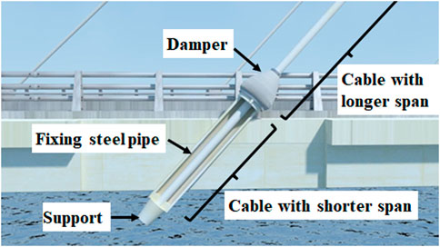
FIGURE 2. Image of cable with damper.

The absolute values of the mode shapes are taken; therefore, the sign of the mode shapes can be ignored. The mode shapes are normalized such that the larger value becomes equal to one.

Let the absolute value of the measured Fourier amplitudes for the ith mode at two points ($x=p_1$ and $x=p_2$) be $\left|V_i^m\left(p_1\right)\right|$ and $\left|V_i^m\left(p_2\right)\right|$ as shown in Figure 3. The measured mode shapes at the two points (${\varphi }_i^m\left(p_1\right)$ and ${\varphi }_i^m\left(p_2\right)$) are defined as follows.

$\left|{\varphi }_i^m\left(p_1\right)\right|=\frac{\left|V_i^m\left(p_1\right)\right|/\left|V_i^m\left(p_2\right)\right|}{max(\left|V_i^m\left(p_1\right)\right|/\left|V_i^m\left(p_2\right)\right|,1)}(\mathrm{22a})$

$\left|{\varphi }_i^m\left(p_2\right)\right|=\frac{1}{max(\left|V_i^m\left(p_1\right)\right|/\left|V_i^m\left(p_2\right)\right|,1)}(\mathrm{22b})$

FIGURE 3

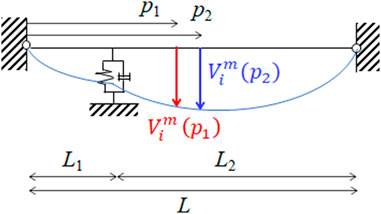
FIGURE 3. Measurement of Fourier amplitudes ($V_i^m\left(p_1\right)$, $V_i^m\left(p_2\right)$ ) at $i$^th mode at two points.

From Eqs 21, 22, the constraint equation, whereby the theoretical mode shapes match the measured mode shapes, becomes as follows.

${\varphi }_i^t\left(p_1\right){\varphi }_i^m\left(p_2\right) - {\varphi }_i^t\left(p_2\right){\varphi }_i^m\left(p_1\right)=0 (i=1, 2,\dots )(23)$

3.3 Method 2FM

Method 2FM is an extended version of Method 2F, and uses mode shapes in addition to natural frequencies. It is assumed that $n$ sets of natural frequencies $f_i^m$, and $n$ sets of mode shapes (${\varphi }_i^m\left(p_1\right)$, ${\varphi }_i^m\left(p_2\right)$) have been measured. The optimization problem in Eq. 24 is solved to simultaneously estimate $4+n$ parameters ($T$, $EI$, $k_u$, $k_v$, and $H_i$, or $T$, $EI$, $k$, $c$, and $H_i$); $G_{2FM}$ is the objective function of Method 2FM.

$minimize G_{2FM}\left(T,EI,k_u,k_v,H_i\right)\begin{array}{c}={\displaystyle \sum }_{i=1}^n\left\{{\left(\text{Re}\left(g_i\right)\right)}^2+{\left(\text{Im}\left(g_i\right)\right)}^2+{\left({\varphi }_i^t\left(p_1\right){\varphi }_i^m\left(p_2\right) - {\varphi }_i^t\left(p_2\right){\varphi }_i^m\left(p_1\right)\right)}^2\right\}\\ (\text{high}-\text{damping rubber damper})\end{array}(\mathrm{24a})$

$minimize G_{2FM}\left(T,EI,k,c,H_i\right)\begin{array}{c}={\displaystyle \sum }_{i=1}^n\left\{{\left(\text{Re}\left(g_i\right)\right)}^2+{\left(\text{Im}\left(g_i\right)\right)}^2{\left({\varphi }_i^t\left(p_1\right){\varphi }_i^m\left(p_2\right) - {\varphi }_i^t\left(p_2\right){\varphi }_i^m\left(p_1\right)\right)}^2\right\}\\ \left(\text{viscous shear damper}\right)\end{array}(\mathrm{24b})$

Because there are $4+n$ unknowns and $3n$ constraint equations, $n$ must at least be equal to two.

4 Numerical Verification

4.1 Overview

The validity of the proposed method was verified by numerical simulation. First, the values of the cable parameters ($\rho$, $A$, $L, L_1, T,$ and $EI$) and damper parameters ($k_u$ and $k_v$, or $k$ and $c$) were assumed. Next, the natural frequencies of the cable with a damper ($\text{Re}\left(f_i^t\right)$) and mode shapes (${\varphi }_i^m\left(p_1\right)$ and ${\varphi }_i^m\left(p_2\right)$) were calculated. Then, the calculated natural frequencies and mode shapes were input into the methods to estimate $T$, $EI$, $k_u$, $k_v$, and $H_i$, or $T$, $EI$, $k$, $c$, and $H_i$. The estimation accuracy was investigated by comparing the estimated values to the assumed values.

4.2 Analytical Conditions

4.2.1 Numerical Models

The cable parameters are listed in Table 1, and the damper parameters are listed in Table 2. These values were set to cover a wide range of cables and dampers. In practical situations, the damper is installed near the girder. Therefore, the damper location, $L_1$, was set to a small value compared with the cable length, $L$.

TABLE 1

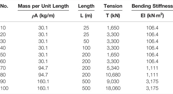
TABLE 1. Cable parameters in numerical verification.

TABLE 2

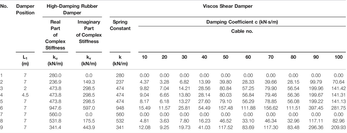
TABLE 2. Damper parameters in numerical verification.

For the high-damping rubber damper, the values of the real part $k_u$ and imaginary part $k_v$ of the complex stiffness $k_i^{\ast }$ are listed in Table 2. For the viscous shear damper, the spring constant $k$ was set to the same value as $\left|k_i^{\ast }\right|$ of the high-damping rubber damper. The damping coefficient $c$ was determined such that the imaginary part of the first mode complex stiffness $\text{Im}(k_1^{\ast }$) becomes similar for the two damper models. Specifically, the damping coefficient $c$ was determined by $=k_v/2\pi f_1$ , where $f_1$ is the first mode natural frequency of the cable with a high-damping rubber damper in the same damper case. The $k$ and $c$ values are listed in Table 2.

By combining ten cable models and nine damper models, 90 numerical models were established. The model number is defined as the sum of the cable number and damper number. For example, model No. 15 consists of cable No. 10 and damper No. 5.

4.2.2 Number of Natural Frequencies and Mode Shapes

Based on the authors’ previous experience on measuring the natural frequencies of a cable with a damper, it is known that there are cases wherein the natural frequencies can be measured only up to the seventh mode (Furukawa et al., 2021b). The natural frequencies of the higher modes are occasionally difficult to measure because the damper dissipates the higher-mode vibration. Therefore, the natural frequencies and mode shapes of the first seven modes were used.

It is assumed that two accelerometers are placed at $p_1=L_1+0.5$ m and $p_2=L_1+$ 1.5 m (Figure 3), and the mode shapes at these points are used in Method 2FM. The accelerometers are placed near the girder considering the efficiency of the inspection work.

4.2.3 Solving Nonlinear Optimization Problem

Because both Methods 2F and 2FM solve the nonlinear least-squares problem, the solution depends on the initial points (initial parameters for unknowns), and there are multiple local minimum solutions. Therefore, this study used the MultiStart algorithm (MathWorks, 2020), wherein the solver attempts to find multiple local minima solutions to a problem by starting from various initial points. The final solution has the smallest objective function value amongst the local minimum solutions. Although there is no guarantee that this algorithm will always find the global minimum solution, it can still find a better solution than the general nonlinear least-squares method while using only one starting point.

The estimation accuracy depends on the number of initial points and the lower and upper bounds of each unknown. This study randomly generated 200 sets of initial points for unknowns. Table 3 indicates the lower and upper bounds of the unknowns in the search for solutions.

TABLE 3

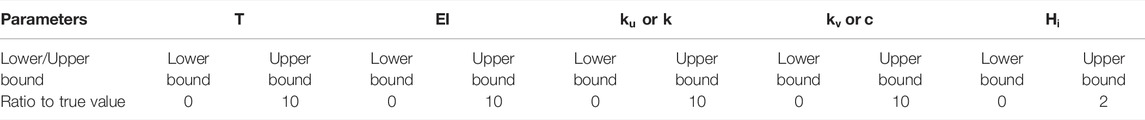
TABLE 3. Solution range when solving optimization problem in numerical verification.

4.3 Estimation Results When Measurement Noise Is Ignored

First, the estimation results without measurement noise were investigated. The estimated results are shown in Figure 4. The horizontal axis is the model number. The vertical axis is the ratio of the estimated value to the true (assumed) value. Notably, a model whose vertical axis value is closer to 1.0 has higher estimation accuracy.

FIGURE 4

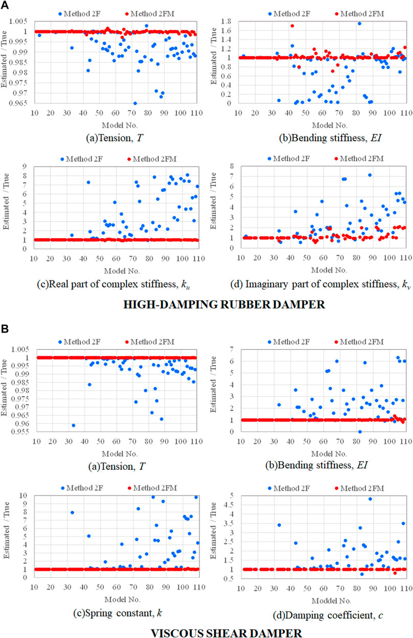
FIGURE 4. Estimation results without measurement noise: (A) high-damping rubber damper; (B) viscous shear damper.

The root mean squares error ratio (RMSER) expressed by Eq. 25 was also calculated for each method.

$\text{RMSER}=\sqrt{\frac{1}{90}{\displaystyle \sum }_{I=1}^{90}{\left(X_I^{estimated}/X_I^{true}-1\right)}^2}(25)$

Here, $I$ is the model number, $X_I^{estimated}$ is the estimated value of model number $I$, and $X_I^{true}$ is the assumed true value of model number $I$. The RMSER was estimated with regard to $T$, $EI$, $k_u$, and $k_v$ for the high-damping rubber damper, and $T$, $EI$, $k$, and $c$ for the viscous shear damper.

4.3.1 Results of Tension Estimation

The tension estimation result for a cable with a high-damping rubber damper is shown in Figure 4Aa. The vertical axis range is 0.96502–1.00645 in Method 2F and 0.99721–1.00160 in Method 2FM. The tension estimation result for a cable with a viscous shear damper is shown in Figure 4Ba. The vertical axis range is 0.95887–1.00000 in Method 2F and 0.99992–1.00008 in Method 2FM. Method 2FM has a smaller estimation error than Method 2F for both damper types.

Table 4 compares the RMSER values. For both damper types, Method 2FM has a smaller RMSER than Method 2F.

TABLE 4

TABLE 4. RMSER of estimation results for high-damping rubber damper in numerical verification.

The above comparison confirms that the estimation accuracy improved with the addition of two-point mode shapes.

Next, a sensitivity analysis was conducted to understand why Method 2FM has higher accuracy compared with Method 2F. Figures 5Aa,Bb show the sensitivity analysis results. Model No. 33 is considered as an example. These figures show how the objective function value in Eq. 17 for Method 2F and Eq. 24 for Method 2FM change when only the tension is variable. The horizontal axis gives the ratio of the value of the tension input into the objective function to the true (assumed) tension. The horizontal axis is set in the range of 0–2.

FIGURE 5

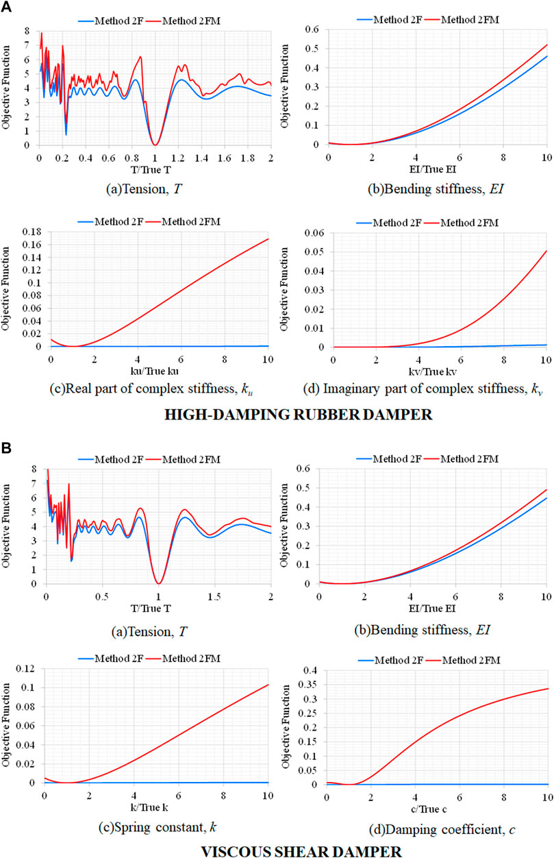
FIGURE 5. Sensitivity analysis results for model No. 33 without measurement noise: (A) high-damping rubber damper; (B) viscous shear damper.

In Figures 5Aa,Ba, the vertical axis value takes the minimum value when the horizontal axis value is equal to one. The vertical axis value rapidly increases as the horizontal axis value departs from one. This indicates that the tension has strong sensitivity to the objective function. The vertical axis value of Method 2FM is larger than that of Method 2F around the horizontal axis value of one. Therefore, the sensitivity of tension is already high in Method 2F, and becomes even higher in Method 2FM.

4.3.2 Results of Bending Stiffness Estimation

The bending stiffness estimation result for the two damper models is shown in Figures 4Ab,Bb. The vertical axis range is 0.00432–1.75065 in Method 2F and 0.70587 to 1.70066 in Method 2FM for cables with a high-damping rubber damper. The vertical axis range is 0.00030–6.30652 in Method 2F and 0.82123–1.35231 in Method 2FM for cables with a viscous shear damper.

Tables 4, 5 compare the RMSER values. For both damper types, Method 2FM has the smaller RMSER.

TABLE 5

TABLE 5. RMSER of estimation results for viscous shear damper in numerical verification.

The bending stiffness estimation accuracy of Method 2F is very low, but the accuracy improved by adding two-point mode shapes. However, some aspects of accuracy, such as the tension accuracy, could not be obtained even with Method 2FM.

The bending stiffness estimation accuracy obtained by Method 2F can be explained as follows. As expressed by Eq. 10, the sensitivity of the bending stiffness $EI$ over the complex natural frequencies $f_i^t$ is low because the $EI$ coefficient is much smaller than the $T$ coefficient in the lower mode (smaller $i$). Therefore, to estimate the bending stiffness with high accuracy, it is necessary to use the natural frequencies of the higher mode (larger $i$). However, because the damper dissipates the higher-mode vibration, the measurement of higher-mode natural frequencies is difficult in practical situations. Therefore, in actual situations, it is difficult to estimate the bending stiffness with high accuracy using Method 2F.

Figures 5Ab,Bb show the sensitivity analysis results for model No. 33 with regard to the bending stiffness. The vertical axis value is minimum when the horizontal axis value is equal to one, but the slope is not sharp as that of tension. The difference between Methods 2F and 2FM is small, which means that the bending stiffness is less sensitive to the objective functions of both methods compared with tension, and adding two-point mode shapes only slightly increases the sensitivity of the bending stiffness.

4.3.3 Results of Damper Parameter Estimation

The damper parameter estimation result for $k_u$, $k_v$, $k$, and $c$, is shown in Figures 4Ac,Ad,Bc,Bd. The vertical axis range of $k_u$ is 0.03726–8.08801 for Method 2F and 0.90686–1.05420 for Method 2FM. The vertical axis range of $k_v$ is 0.55892–7.12971 for Method 2F and 0.56344–2.08867 for Method 2FM. The range of the vertical axis of $k$ is 0.99991–9.81214 for Method 2F and 0.98322–1.10842 for Method 2FM. The range of the vertical axis of $c$ is 0.73836–4.82487 for Method 2F and 0.80157–1.00750 for Method 2FM.

Table 4 compares the RMSER values. For both damper types, Method 2FM has the smaller RMSER.

The accuracy of Method 2F is inferior, but that of Method 2FM dramatically improves with the addition of two-point mode shapes. Hence, the superiority of Method 2FM over Method 2F is clear.

Figures 5Ac,Ad,Bc,Bd show the sensitivity analysis results for model No. 33 with regard to $k_u$, $k_v$, $k$, and $c$. The vertical value and slope of Method 2F are much smaller than those of Method 2FM, which indicates that the sensitivity of Method 2F is somewhat small, and it is impossible to obtain acceptable damper parameter estimation results with Method 2F. The addition of two-point mode shapes has a considerably more pronounced effect on the damper parameters compared with the tension and bending stiffness.

4.4 Effect of Measurement Noise on Estimation Accuracy

4.4.1 Analysis Condition

When measuring the acceleration of an actual bridge cable, the natural frequencies and mode shapes always contain measurement noise. Therefore, this section discusses the effect of measurement noise on the estimation accuracy. The natural frequencies with measurement noise can be calculated using the approach proposed by Thyagarajan et al. (1998). Artificial measurement noise is added to the theoretical natural frequencies and mode shapes.

$f_i^{noise}=(1+\eta rand)\text{Re}\left(f_i^t\right) i=1, 2,\dots (26)$

${\varphi }_i^{m\_noise}\left(p_1\right)=(1+\eta rand){\varphi }_i^t\left(p_1\right) i=1, 2,\dots (\mathrm{27a})$

${\varphi }_i^{m\_noise}\left(p_2\right)=(1+\eta rand){\varphi }_i^t\left(p_2\right) i=1, 2,\dots (\mathrm{27b})$

where $f_i^{noise}, {\varphi }_i^{m\_noise}\left(p_1\right),$ and ${\varphi }_i^{m\_noise}\left(p_2\right)$ denote the natural frequencies and mode shapes of the $i$^th mode with artificial measurement noise, $\eta$ is the measurement noise ratio, and $rand$ is a uniform random number between -1 and 1. The measurement noise ratio $\eta$ of 0.01, 0.02, and 0.03 was considered, and different random numbers were generated for the natural frequencies and two-point mode shapes of each mode.

The tension, bending stiffness, and damper parameters were estimated using Methods 2F and 2FM by inputting the natural frequencies and mode shapes with measurement noise.

4.4.2 Estimation Results

Because the estimation accuracy depends on the random numbers generated for each natural frequency and mode shape, the average value of ten sets with measurement noise was used for estimation by iteratively calculating Eq. 26, Eq. 27 for 10 times.

The RMSER of the estimated tension, bending stiffness, and two damper parameters for a cable with a high-damping rubber damper and viscous shear damper are shown in Figure 6. The results for $\eta =0$ represent the case without measurement noise.

FIGURE 6

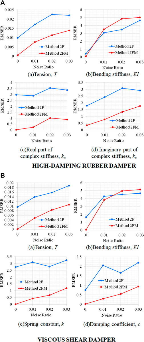
FIGURE 6. RMSER of estimation results for various measurement noise ratios: (A) high-damping rubber damper; (B) viscous shear damper.

With regard to tension, Method 2FM has a much smaller RMSER compared with Method 2F for both damper types (Figures 6Aa,Ba). By adding two-point mode shapes, the tension estimation accuracy improved even with measurement noise.

With regard to the bending stiffness, the RMSER of Method 2FM is similar to that of Method 2F (Figures 6Ab,Bb), and the RMSER is very large in both methods compared with tension. Hence, the estimated bending stiffness with measurement noise is not reliable.

With regard to the damper parameters, the RMSER of Method 2FM is much smaller than that of Method 2F (Figures 6Ac,Ad,Bc,Bd), and decreased with the addition of two-point mode shapes.

4.5 Sensitivity analysis

Sensitivity analysis was conducted to understand why the accuracy of the tension and damper parameters improved while the bending stiffness accuracy did not improve by adding mode shapes. Figure 7 shows the sensitivity analysis results with measurement noise. Model No. 33 is considered as an example. The natural frequencies and mode shapes with measurement noise were input into the calculation of the objective functions. The ratio of the measurement noise in the natural frequencies and mode shapes was set to 0.01 (1%) for all modes. The theoretical natural frequency was multiplied by 1.01 ($1.01\text{Re}\left(f_i^t\right)$) and input to Eq. 17, Eq, 24. For the mode shapes, the theoretical values of ${\varphi }_i^t\left(p_1\right)$ and ${\varphi }_i^t\left(p_2\right)$ were multiplied by 1.0, 1.01 (${\varphi }_i^t\left(p_1\right)$, and $1.01{\varphi }_i^t\left(p_2\right)$) and input into Eq. 24.

FIGURE 7

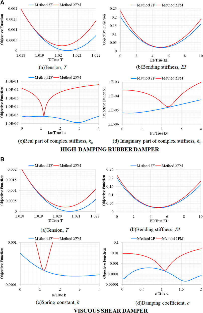
FIGURE 7. Sensitivity analysis results for model No. 33 with measurement error of 1%: (A) high-damping rubber damper; (B) viscous shear damper.

The sensitivity analysis results for tension are shown in Figures 7Aa,Ba. The horizontal axis value where the vertical axis value is minimum shifted from one owing to the measurement noise. For example, in Eq. 9a, the vertical axis value is minimum when the horizontal axis value is 1.0206 in Method 2F. This means that the tension must be 1.0206 times larger such that the natural frequencies increase by 1%. In both damper types, the horizontal axis value with the minimum vertical value is closer to one in Method 2FM compared with Method 2F. This means that the solution of the tension estimation in Method 2FM is less likely to be affected by measurement noise, and Method 2FM is more robust than Method 2F.

The sensitivity analysis results for the bending stiffness are shown in Figures 7Ab,Bb. In both methods, the horizontal axis value with the minimum vertical value is approximately equal to five for both damper types. This means that the bending stiffness must be approximately five times larger such that the natural frequencies increase by 1%. As expressed by Eq. 10, the sensitivity of the bending stiffness $EI$ over the complex natural frequencies $f_i^t$ is low because the $EI$ coefficient is much smaller than the $T$ coefficient in the lower mode (smaller $i$). Because the sensitivity of the bending stiffness against the natural frequency is very low, the solution of the bending stiffness estimation is largely affected by the measurement noise in Method 2F. Adding mode shapes did not improve the bending stiffness accuracy under the condition with measurement noise.

The sensitivity analysis results for the damper parameters ($k_u$, $k_v$, $k$, and $c$) are shown in Figures 7Ac,Ad,Bc,Bd. The vertical axis is displayed in the logarithmic scale. The difference between Methods 2F and 2FM is very clear. Method 2FM has a clear minimum value at the horizontal axis value closer to one for $k_u$, $k$, and $c$. For example, the minimum vertical value of the horizontal axis is 1.14 in Method 2FM and approximately 2.9 in Method 2F, as shown in Figure 7Ac. The reason for this is that the sensitivity of these damper parameters to the natural frequency is low, while the sensitivity to the mode shapes is high. The solution of the damper parameters in Method 2F is strongly affected by the measurement noise, and a reliable solution is difficult to obtain. In contrast, Method 2FM is less likely to be affected by measurement noise, and is therefore much more robust for $k_u$, $k$, and $c$ compared with Method 2F. As shown in Figure 7Ad, even with Method 2FM, $k_v$ is more likely to be affected by measurement noise compared with $k_u$, $k$, and $c$.

4.6 Summary

The validity of the newly proposed Method 2FM was numerically verified by comparing the estimation results to those obtained by the previously proposed Method 2F.

First, the estimation results were compared under the condition without measurement noise.

The tension estimation accuracy is already high in Method 2F but further improves in Method 2FM by the addition of two-point mode shapes. With regard to the bending stiffness and damper parameters, Method 2FM has higher estimation accuracy, but estimation accuracy as high as the tension estimation accuracy cannot be obtained. The sensitivity analysis confirms that the sensitivity of damper parameters to the objective function dramatically increases with the addition of modal shapes.

The effect of measurement noise on the estimation accuracy was investigated. The newly proposed Method 2FM has a smaller RMSER for the tension and damper parameters compared with Method 2F. The sensitivity analysis confirms that Method 2FM is less likely to be affected by measurement noise and more robust for tension and damper parameter estimation compared with Method 2F. The RMSER of the bending stiffness is large for both methods, and reliably estimating the bending stiffness was found to be difficult under the condition with measurement noise.

Based on the above findings, this study concluded that Method 2FM is more versatile than Method 2F.

5 Experimental Verification

5.1 Experimental Conditions

This section describes the experimental validation of the proposed method. The experimental setting is shown in Figures 8A,B. The experiment was conducted using a horizontal cable with a length of 61.8 m. The distance between the two ends was considered as the cable length. A load cell was installed at the right end, and the tension value of the load cell was considered as the true tension value. The cable was hit with a hammer between the damper position and the right end. The acceleration histories were measured by piezoelectric accelerometers magnetically attached to the cable. The natural frequencies were measured by reading the peak frequencies of the acceleration Fourier spectra. The mode shapes were calculated from the acceleration Fourier amplitude at the natural frequencies.

FIGURE 8

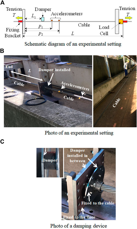
FIGURE 8. Experimental setting: (A) schematic diagram of experimental setting; (B) photo of experimental setting; (C) photo of damping device.

The damper was placed at a distance $L_1$ from one end. Figure 8C shows a photo of the damper device. A rectangular steel plate with a circular hole for the cable to pass through was fixed to the floor. The cable was not in contact with the steel plate. A disk-shaped steel plate with a circular hole for the cable to pass through was fixed to the cable. The damper was installed between the rectangular steel plate and the disk-shaped steel plate. The rectangular steel plate and disk-shaped steel plate were installed in parallel.

The cable parameters are listed in Table 6. A prestressed steel strand was used as the cable because it is used in actual bridge cables.

TABLE 6

TABLE 6. Cable parameters in experimental verification.

The damper parameters are listed in Table 7. Three high-damping rubber dampers were used.

TABLE 7

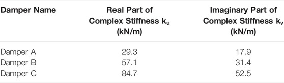
TABLE 7. Damper parameters in experimental verification.

The test cases are listed in Table 8. Cases No. 1–13 are cases with a tension of approximately 180 kN. Cases No. 14–26 are cases with a tension of approximately 380 kN. Cases No. 1 and 14 are cases without a damper. Four cases were considered for each tension and damper combination with regard to the damper position.

TABLE 8

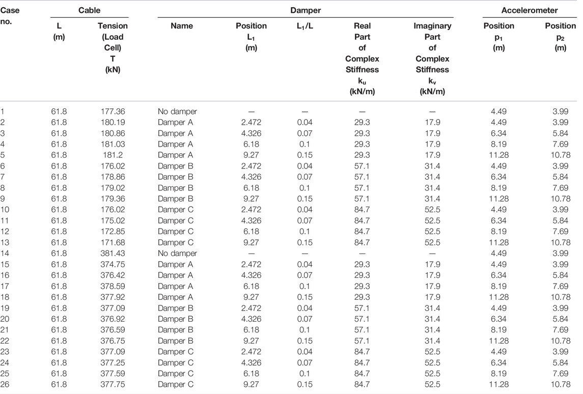
TABLE 8. Test cases in experimental verification.

In the solution of the optimization problem using the MultiStart algorithm, this study randomly generated 200 sets of initial points for the unknowns to avoid a local minimum solution. Table 9 presents the lower and upper bounds of the unknowns in the search for solutions. The lower bounds were set to zero for all parameters. The upper bound of tension was set to ten times the true value. The upper bound of the bending stiffness was set to ten times the design value. The upper bounds of the damper parameters were not limited because the damper stiffness was found to have amplitude-dependency and frequency-dependency, and the values are different to the design values in Table 7, as will be explained later. Regarding the ratio of the imaginary part to the real part of the complex natural frequencies, the upper value was set to 0.019. The damping factor of each mode was evaluated using the half-power method, and 0.019 was set as the upper bound.

TABLE 9

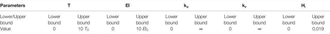
TABLE 9. Solution range when solving optimization problem in experimental verification ($T_0$, tension measured by load cell in Table 5(c); $E{I}_0$, design value in catalog listed in Table 5(a)).

Table 10 lists the first to seventh measured natural frequencies, for which the order was assigned in ascending order based on the measured peak frequencies. Table 11 lists the first to seventh measured mode shapes with the location of two measurement points (p₁ and p₂).

TABLE 10

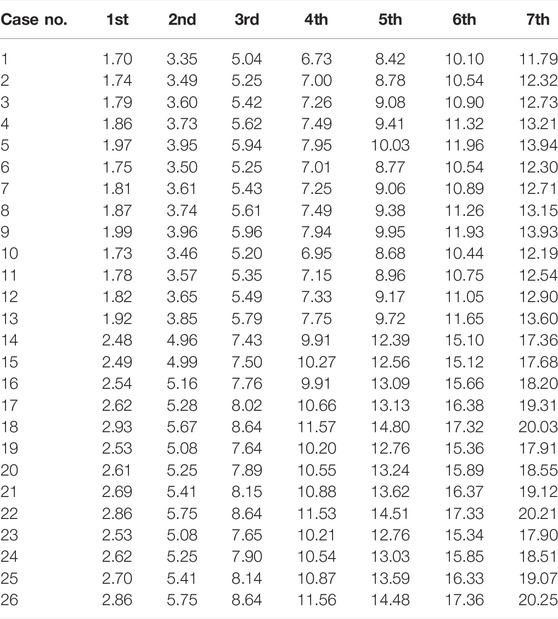
TABLE 10. First to seventh measured natural frequencies in ascending order (Hz).

TABLE 11

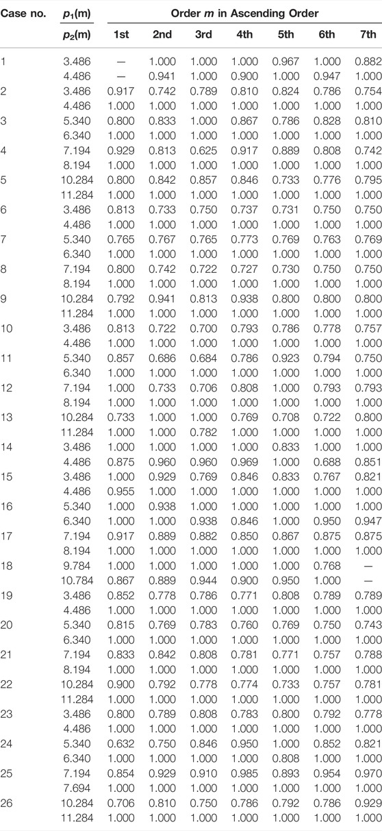
TABLE 11. First to seventh measured mode shapes in ascending order of $m$ (top: ${\varphi }_i^m\left(p_1\right)$; bottom: ${\varphi }_i^m\left(p_2\right)$).

5.2 Estimation Results

The measured natural frequencies listed in Table 10 were input into Methods 2F and 2FM, and the mode shapes listed in Table 11 were input into Method 2FM.

5.2.1 Results of Tension Estimation

Figure 9A shows the tension estimation results. The horizontal axis is the case number, and the vertical axis is the ratio of the estimated tension to the true tension measured by a load cell. Table 12 compares the RMSER of tension.

FIGURE 9

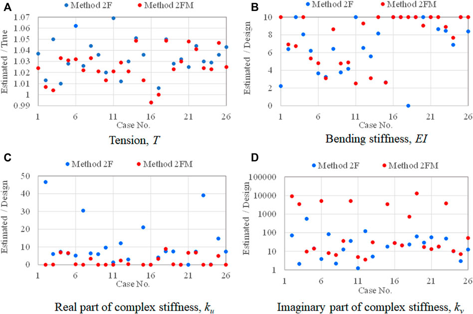
FIGURE 9. Estimation results obtained by experiments: (A) tension, T; (B) bending stiffness, EI; (C) real part of complex stiffness, k_u; (D) imaginary part of complex stiffness.

TABLE 12

TABLE 12. RMSER of estimated tension in experimental verification.

The vertical axis value for Method 2F is between 0.993 and 1.069. Method 2F has high accuracy, but the estimation error of Method 2F for case Nos. 11 and 14 exceeds 5%. In contrast, the vertical axis value for Method 2FM is between 0.993 and 1.048. The estimation error of Method 2FM is smaller than 5% for all cases, and the RMSER of Method 2FM is smaller than that of Method 2F.

In the numerical verification considering the measurement noise, the same measurement noise ratio was assumed for the natural frequencies and the mode shapes. The tension estimation error decreased significantly by adding the mode shapes in the numerical verification. However, in the experimental verification, the tension estimation error did not decrease significantly by adding the mode shapes. It is considered that the mode shape contains more measurement error than the natural frequencies in the experiment. The accuracy of the mode shapes depends on the measurement position. It is possible that the damper affects the accuracy of the mode shapes if the accelerometers are placed near the damper. Therefore, it is found necessary to investigate appropriate measurement positions for the mode shapes from the viewpoint of the tension estimation accuracy.

5.2.2 Results of Bending Stiffness Estimation

Figure 9B shows the bending stiffness estimation results. Both methods did not obtain reliable results. As discussed in the previous section, measurement noise is one reason for the low estimation accuracy.

5.2.3 Results of Damper Parameter Estimation

Figures 9C,D shows the estimation results for cases other than tension estimation. The vertical axis in Figure 9D is displayed in the logarithmic scale because the range is very wide. Both methods did not obtain reliable results.

In the numerical verification discussed in the previous section, Method 2FM estimated the damper parameters with satisfactory accuracy. However, in the experiment, low damper parameter estimation accuracy was obtained with Method 2FM. This is attributed to the modeling error of the damper. To confirm this, the load–displacement relationship of damper B was obtained by an element test under various displacement amplitudes and various frequencies. Figure 10 shows the load–displacement relationship of damper B. Figure 10A shows that the damper has amplitude-dependency, and Figure 10B shows that the damper has frequency-dependency. However, the damper was modeled as a high-damping rubber damper whose complex stiffness is constant regardless of the displacement amplitude and frequency (Eq. 12a), because the damper is commercially available as a high-damping rubber damper. Hence, the low accuracy of damper parameter estimation is attributed to the modeling error of the damper’s complex stiffness.

FIGURE 10

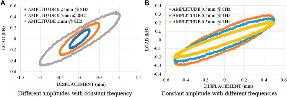
FIGURE 10. Amplitude-dependency and frequency-dependency of load–displacement relationship of damper used in element test (damper B): (A) different amplitudes with constant frequency; (B) constant amplitude with different frequencies.

Equation 12a is a simplified design equation for determining appropriate damper parameters and may not perfectly express the damper’s dynamic characteristics. Therefore, it is necessary to develop a new equation of complex stiffness that can accurately express the dynamic characteristics of the damper to estimate the damper parameters with high accuracy.

Furthermore, the proposed method ignores the effect of damper mass. In the future study, it is necessary to investigate the effect of damper mass on the estimation accuracy and to improve a damper model.

Although the damper’s complex stiffness and effect of damper mass could not be modeled exactly, the tension estimation error was within 5% owing to the stronger sensitivity of tension and lower sensitivity of the damper parameters against the vibration characteristics. It is expected that the tension and damper parameter estimation accuracy can further improve by adopting an appropriate damper model.

6 Conclusion

This paper proposes a new method (Method 2FM) for estimating the tension and bending stiffness of cable and damper parameters based on the natural frequencies and two-point mode shapes. Method 2FM is an updated version of the previously proposed Method 2F, which only uses the natural frequencies. The novelty of Method 2FM is the use of mode shapes measured at only two points, in addition to the natural frequencies. Only two accelerometers are needed, and measurement at multiple locations throughout the cable is not required.

Firstly, the validity of the previously and newly proposed methods was numerically verified. Ninety numerical models were established with ten cable models and nine damper models for two damper types: a high-damping rubber damper and a viscous shear damper.

Method 2FM improves the tension estimation accuracy of Method 2F through the addition of two-point mode shapes. Method 2FM has higher tension estimation accuracy than Method 2F, even with measurement noise. Moreover, the tension estimation result is less likely to be affected by measurement noise compared with other parameters.

The bending stiffness estimation accuracy improved with Method 2FM when there was no measurement noise. However, reliable bending stiffness estimation is difficult with measurement noise because the bending stiffness is less sensitive to the vibration characteristics of the lower modes.

With regard to damper parameter estimation, the accuracy of Method 2F is very low, even in the case without measurement noise. However, the accuracy dramatically improves in Method 2FM, and the sensitivity of the damper parameters against the objective function dramatically increases with the addition of mode shapes.

The validity of the proposed method was experimentally verified using a cable with a length of 61.8 m. A high-damping rubber damper was installed, and 26 cases were prepared by changing the cable tension, damper models, and damper position.

The tension estimation accuracy of Method 2FM is higher than that of Method 2F, and the maximum estimation error is 4.8%. For method 2FM, the tension estimation error is within 5%. It was found necessary to investigate appropriate measurement positions for the mode shapes from the viewpoint of the tension estimation accuracy.

Both models did not estimate the damper parameters with high accuracy, possibly owing to the modeling error of the damper’s complex stiffness. Because a high-damping rubber damper was used in the experiment, the damper’s complex stiffness was set to constant values regardless of the vibration amplitude and vibration frequencies. However, the element test revealed that the actual damper was amplitude-dependent and frequency-dependent. Although the damper’s complex stiffness could not be modeled exactly, a tension estimation error within 5% was achieved owing to the stronger sensitivities of tension and lower sensitivity of damper parameters to the vibration characteristics. It is expected that the tension and damper parameter estimation accuracy can further improve by adopting an appropriate damper model.

The numerical and experimental verifications demonstrate the superiority of Method 2FM over Method 2F, and it is possible to estimate the cable tension without detaching the damper. The fact that the cable does not have to be detached is a great advantage in terms of work efficiency.

This study proposed a deterministic estimation method. The cable’s tension and bending stiffness and two damper parameters are estimated from the natural frequencies and the two-point mode shapes, assuming that the mass per unit length and length of cable, and damper position are given correctly. However, these parameters contain uncertainty. In addition, the measured natural frequencies and the two-point mode shapes contain uncertainty. Therefore, it is desirable to consider the uncertainty of the input parameters. In the next step, the authors would like to develop a probabilistic estimation method based on Bayesian inference.

In future work, the authors will attempt to improve the estimation accuracy of both the tension and damper parameters by developing an appropriate damper model. Moreover, the authors will investigate the effect of damper mass on the estimation accuracy and improve the damper model. Furthermore, verification will be carried out using measurement data obtained for actual bridges.

Data Availability Statement

The original contributions presented in the study are included in the article, further inquiries can be directed to the corresponding author.

Author Contributions

AF developed the proposed methods, wrote the source code for estimating the cable tension, and carried out the numerical analysis. SS carried out the numerical analysis. RK conducted the verification experiment.

Conflict of Interest

RK was employed by Kobelco Wire Company Ltd.

The remaining authors declare that the research was conducted in the absence of any commercial or financial relationships that could be construed as a potential conflict of interest.

Publisher’s Note

All claims expressed in this article are solely those of the authors and do not necessarily represent those of their affiliated organizations, or those of the publisher, the editors and the reviewers. Any product that may be evaluated in this article, or claim that may be made by its manufacturer, is not guaranteed or endorsed by the publisher.

References

Chen, C.-C., Wu, W.-H., Chen, S.-Y., and Lai, G. (2018). A Novel Tension Estimation Approach for Elastic Cables by Elimination of Complex Boundary Condition Effects Employing Mode Shape Functions. Eng. Struct. 166, 152–166. doi:10.1016/j.engstruct.2018.03.070

CrossRef Full Text | Google Scholar

Chen, C.-C., Wu, W.-H., Leu, M.-R., and Lai, G. (2016). Tension Determination of Stay Cable or External Tendon with Complicated Constraints Using Multiple Vibration Measurements. Measurement 86, 182–195. doi:10.1016/j.measurement.2016.02.053

CrossRef Full Text | Google Scholar

Feng, Z., Wang, X., and Chen, Z. (2010). A Method of Fundamental Frequency Hybrid Recognition for Cable Tension Measurement of Cable-Stayed Bridges. 8th IEEE International Conference on Control and Automation, Xiamen, China, June 11, 2010. doi:10.1109/icca.2010.5524186

CrossRef Full Text | Google Scholar

Foti, F., Geuzaine, M., and Denoel, V. (2020). On the Identification of the Axial Force and Bending Stiffness of Stay Cables Anchored to Flexible Supports. Appl. Math. Model. 92, 798–828.

Google Scholar

Furukawa, A., Hirose, K., and Kobayashi, R. (2021b). Tension Estimation Method for Cable with Damper and its Application to Real Cable-Stayed Bridge, Proceedings of the 9th International Conference on Experimental Vibration Analysis for Civil Engineering Structures, (Online), September 15, 2021. Paper No. S8-1.

Google Scholar

Furukawa, A., Hirose, K., and Kobayashi, R. (2021a). Tension Estimation Method for Cable with Damper Using Natural Frequencies. Front. built Environ. 7, 603857. doi:10.3389/fbuil.2021.603857

CrossRef Full Text | Google Scholar

Furukawa, A., Suzuki, S., and Kobayashi, R. (2022b). Tension Estimation Method for Cable with Damper Using Natural Frequencies with Uncertain Modal Order. Front. built Environ. 8, 812999. doi:10.3389/fbuil.2022.812999

CrossRef Full Text | Google Scholar

Furukawa, A., Yamada, S., and Kobayashi, R. (2022a). Tension Estimation Methods for Two Cables Connected by an Intersection Clamp Using Natural Frequencies. J. Civ. Struct. Health Monit. 12, 339–360. doi:10.1007/s13349-022-00548-6

CrossRef Full Text | Google Scholar

Gan, Q., Huang, Y., Wang, R. O., and Rao, R. (2019). Tension Estimation of Hangers with Shock Absorber in Suspension Bridge Using Finite Element Method. J. Vibroengineering 21 (3), 587–601. doi:10.21595/jve.2018.20054

CrossRef Full Text | Google Scholar

Haji Agha Mohammad Zarbaf, S. E., Norouzi, M., Allemang, R., Hunt, V., Helmicki, A., and Venkatesh, C. (2018). Vibration-based Cable Condition Assessment: A Novel Application of Neural Networks. Eng. Struct. 177, 291–305. doi:10.1016/j.engstruct.2018.09.060

CrossRef Full Text | Google Scholar

Hou, J., Li, C., Jankowski, Ł., Shi, Y., Su, L., Yu, S., et al. (2020). Damage Identification of Suspender Cables by Adding Virtual Supports with the Substructure Isolation Method. Struct. Control Health Monit. 28 (3), e2677. doi:10.1002/stc.2677

CrossRef Full Text | Google Scholar

Izzi, M., Caracoglia, L., and Noè, S. (2016). Investigating the Use of Targeted-Energy-Transfer Devices for Stay-Cable Vibration Mitigation. Struct. Control Health Monit. 23, 315–332. doi:10.1002/stc.1772

CrossRef Full Text | Google Scholar

Javanbakht, M., Cheng, S., and Ghrib, F. (2019). Control-oriented Model for the Dynamic Response of a Damped Cable. J. Sound Vib. 442, 249–267. doi:10.1016/j.jsv.2018.10.036

CrossRef Full Text | Google Scholar

Kim, B. H., and Park, T. (2007). Estimation of Cable Tension Force Using the Frequency-Based System Identification Method. J. Sound Vib. 304, 660–676. doi:10.1016/j.jsv.2007.03.012

CrossRef Full Text | Google Scholar

Krenk, S. (2000). Vibrations of a Taut Cable with an External Damper. ASME, J. Appl. Mech. 67, 772–776. doi:10.1115/1.1322037

CrossRef Full Text | Google Scholar

Lazar, I. F., Neild, S. A., and Wagg, D. J. (2016). Vibration Suppression of Cables Using Tuned Inerter Dampers. Eng. Struct. 122, 62–71. doi:10.1016/j.engstruct.2016.04.017

CrossRef Full Text | Google Scholar

Li, S., Wang, L., Wang, H., Shi, P., Lan, R., Wu, C., et al. (2021). An Accurate Measurement Method for Tension Force of Short Cable by Additional Mass Block. Adv. Mater. Sci. Eng. 2021, 1–10. Article ID 6622628. doi:10.1155/2021/6622628

CrossRef Full Text | Google Scholar

Ma, L. (2017). A Highly Precise Frequency-Based Method for Estimating the Tension of an Inclined Cable with Unknown Boundary Conditions. J. Sound Vib. 409, 65–80. doi:10.1016/j.jsv.2017.07.043

CrossRef Full Text | Google Scholar

Ma, L., Xu, H., Munkhbaatar, T., and Li, S. (2021). An Accurate Frequency-Based Method for Identifying Cable Tension while Considering Environmental Temperature Variation. J. Sound Vib. 490, 1–16. Article ID 115693. doi:10.1016/j.jsv.2020.115693

CrossRef Full Text | Google Scholar

MathWorks (2020). MATLAB Documentation, MultiStart. Avabilable: https://jp.mathworks.com/help/gads/ multistart.html (Accessed April 30, 2021).

Google Scholar

Pacheco, B. M., Fujino, Y., and Sulekh, A. (1993). Estimation Curve for Modal Damping in Stay Cables with Viscous Damper. J. Struct. Eng. 119 (6), 1961–1979. doi:10.1061/(asce)0733-9445(1993)119:6(1961)

CrossRef Full Text | Google Scholar

Shan, D., Zhou, X., and Khan, I. (2019). Tension Identification of Suspenders with Supplemental Dampers for Through and Half-Through Arch Bridges Under Construction, ASCE. J. Struct. Eng. 145 (3), 040182565-1 to 040182565-11. doi:10.1061/(asce)st.1943-541x.0002255

CrossRef Full Text | Google Scholar

Shi, X., and Zhu, S. (2018). Dynamic Characteristics of Stay Cables with Inerter Dampers. J. Sound Vib. 423, 287–305. doi:10.1016/j.jsv.2018.02.042

CrossRef Full Text | Google Scholar

Shinke, T., Hironaka, K., Zui, H., and Nishimura, H. (1980). Practical Formulas for Estimation of Cable Tension by Vibration Method. Proc. Jpn. Soc. Civ. Eng. 1980, 25–32. (In Japanese). doi:10.2208/jscej1969.1980.294_25

CrossRef Full Text | Google Scholar

Shinko Wire Company, Ltd, (2020). Tension Measuring Technique for Outer Cables. (In Japanese) Avabilable: http://www.shinko-wire.co.jp/products/vibration.html (Accessed April 30, 2021).

Google Scholar

Tabatabai, H., and Mehrabi, A. B. (2000). Design of Mechanical Viscous Dampers for Stay Cables. J. Bridge Eng. 5 (2), 114–123. doi:10.1061/(asce)1084-0702(2000)5:2(114)

CrossRef Full Text | Google Scholar

Thyagarajan, S. K., Schulz, M. J., Pai, P. F., and Chung, J. (1998). Detecting Structural Damage Using Frequency Response Functions. J. Sound Vib. 210, 162–170. doi:10.1006/jsvi.1997.1308

CrossRef Full Text | Google Scholar

Yamagiwa, I., Utsuno, H., Endo, K., and Sugii, K. (2000). Identification of Flexural Rigidity and Tension of the One-Dimensional Structure by Measuring Eigenvalues in Higher Order. Trans. JSME(C) 66 (649), 2905–2911. (In Japanese). doi:10.1299/kikaic.66.2905

CrossRef Full Text | Google Scholar

Yan, B., Chen, W., Dong, Y., and Jiang, X. (2020). Tension Force Estimation of Cables with Two Intermediate Supports. Int. J. Struct. Stab. Dyn. 20 (3), 2050032-1 to 2050032-23. doi:10.1142/s0219455420500327

CrossRef Full Text | Google Scholar

Yan, B., Chen, W., Yu, J., and Jiang, X. (2019). Mode Shape-Aided Tension Force Estimation of Cable with Arbitrary Boundary Conditions. J. Sound Vib. 440, 315–331. doi:10.1016/j.jsv.2018.10.018

CrossRef Full Text | Google Scholar

Zarbaf, S. E. H. A. M., Norouzi, M., Allemang, R., Hunt, V., and Helmicki, A. (2017). Stay Cable Tension Estimation of Cable-Stayed Bridges Using Genetic Algorithm and Particle Swarm Optimization. J. Bridge Eng. 22 (10), 05017008-1 to 05017008-9. doi:10.1061/(asce)be.1943-5592.0001130

CrossRef Full Text | Google Scholar

Zui, H., Shinke, T., and Namita, Y. (1996). Practical Formulas for Estimation of Cable Tension by Vibration Method. J. Struct. Eng. 122 (6), 651–656. doi:10.1061/(asce)0733-9445(1996)122:6(651)

CrossRef Full Text | Google Scholar