Deep deterministic policy gradient and graph convolutional network for bracing direction optimization of grid shells

In this paper, we propose a method for bracing direction optimization of grid shells using a Deep Deterministic Policy Gradient (DDPG) and Graph Convolutional Network (GCN). DDPG allows simultaneous adjustment of variables during the optimization process, and GCN allows the DDPG agent to receive data representing the whole structure to determine its actions. The structure is interpreted as a graph where nodes, element properties, and internal forces are represented by the node feature matrix, adjacency matrices, and weighted adjacency matrices. DDPG agent is trained to optimize the bracing directions. The trained agent can find sub-optimal solutions with moderately small computational cost compared to the genetic algorithm. The trained agent can also be applied to structures with different sizes and boundary conditions without retraining. Therefore, when various types of braced grid shells have to be considered in the design process, the proposed method can significantly reduce computational cost for structural analysis.

1 Introduction

Structural optimization aims to obtain the best design variables that minimize/maximize an objective function under specified constraints (Christensen and Klarbring, 2009). For discrete structures, such as trusses and frames, typically, the design variables are cross-sectional properties, nodal locations and/or nodal connectivity (Ohsaki and Swan, 2002). Finding the best nodal locations is generally called geometry optimization, and the determination of nodal connectivity is called topology optimization. Structural optimization is important in early-stage design of large-span grid shells because their structural performance depends significantly on the shape and topology (Ohsaki, 2010). An optimization problem for grid shells can be formulated to maximize the stiffness against static loads through minimization of the compliance (i.e., elastic strain energy). Examples of such formulation can be found in Refs. (Topping, 1983; Wang et al., 2002; Kociecki and Adeli, 2015).

In topology optimization of grid shells where bracing directions are to be optimized, the optimization problem can be formulated as a combinatorial problem and solved using heuristic approaches such as genetic algorithm (GA) and simulated annealing without utilizing gradient information (Dhingra and Bennage, 1995; Ohsaki, 1995; Kawamura et al., 2002). While this approach allows for simple implementation, it requires many evaluations of the structural response and therefore has a high computational cost especially for structures made of many elements (i.e., many design variables). In addition, the topology optimization problem to minimize compliance can be formulated as mixed-integer programming (MIP) which is practical for small- to medium-size optimization problems due to computational cost (Kanno and Fujita, 2018). Recent advances in MINLP enable to solve very large mixed-integer problems with quadratic and/or bilinear objective function and constraints. However, both heuristic and mathematical programming approaches do not allow the use of knowledge acquired from previously obtained solutions for similar structural configurations.

In recent years, machine learning (ML) approaches have been applied to structural optimization problems. ML can be classified into supervised learning, unsupervised learning, and reinforcement learning (RL). A supervised learning model learns to map (predict or classify) given input instances to specific output domains using sample data for training. Examples of this method for structural optimization can be found in (Berke et al., 1993; Hung et al., 2019; Mai et al., 2021). An unsupervised learning model learns to capture relationships between instances (data). Examples of unsupervised learning are t-distributed stochastic neighbor embedding (t-SNE) (van der Maaten and Hinton, 2008) and k-means clustering (MacQueen, 1967). Jeong and Yoshimura (Jeong and Yoshimura, 2002) also applied an improved unsupervised learning method to multi-objective optimization of plane trusses. Applications of unsupervised learning methods for structural design and structural damage detection can be found in (Eltouny and Liang, 2021; Puentes et al., 2021).

RL is a type of ML that has been developed from optimal control and dynamic programming (Sutton and Andrew, 2018). In RL, a model, or agent, is allowed to interact with an environment. The agent adjusts its policy to take actions according to given reward signals, which are designed to encourage the agent to do actions that change the environment into a desirable state such as winning a game or obtaining solutions to problems. RL has been successfully applied to various problems such as playing arcade games (Mnih et al., 2013) and controlling vehicles (Yu et al., 2019).

Deep Deterministic Policy Gradient (DDPG) (Lillicrap et al., 2016) is a type of RL algorithm that uses two neural networks (NN) (Rosenblatt, 1958; Ivakhnenko, 1968; Goodfellow et al., 2016) as an agent. The DDPG can be used in an environment where multiple agent actions are needed. Kupwiwat and Yamamoto (Kupwiwat and Yamamoto, 2020) studied various RL algorithms, using NNs as agents, and found that DDPG can be effectively applied to the geometry optimization problem of grid shell structures. However, the agents can only observe a constant number of inputs. Therefore, when structural dimensions are changed, it is difficult for the agents to detect the change of structural characteristics.

Hayashi and Ohsaki (Hayashi and Ohsaki, 2021) proposed a combined method of RL and graph representation for binary topology optimization of planar trusses. Graph representation allows an RL agent to observe the whole structure by transforming the structure into graph data consisting of nodes (vertices) and elements (edges) and implementing repetitive graph embedding operations to transmit signals of adjacent nodes and elements for estimating accumulated rewards associated with each action. Zhu et al. (2021) studied the applicability of RL and graph representation for stochastic topology generation of stable trusses which can be further used as initial structures for other topology optimization algorithms.

Graph neural networks are types of NNs, specifically designed for working with graph data. Graph Convolutional Network (GCN) (Kipf and Welling, 2017) is a class of graph neural networks that uses a convolution operator to process graph signals to the output domain. GCN has been successfully applied to problems such as node classification (Kipf and Welling, 2017) and link prediction (Kipf and Welling, 2016).

This paper proposes methods for the bracing directions optimization of grid shell structures for minimizing the strain energy using DDPG and GCN. The RL agent is trained to optimize the bracing directions from initial randomly generated directions. The proposed method is considered a part of the early-stage design of grid shells. The method takes an input the shape of the grid-shell which must be pre-determined. Bracing direction optimization can reduce the structure’s strain energy without affecting the appearance of the shape because the braces are typically covered by finishing or ceiling. This paper is organized as follows: Section 2 gives the optimization formulations. Sections 3, 4 introduce existing approaches of GCN and a type of RL named DDPG, respectively. Section 5 explains the novelty of this research consisting of the vectors and matrices utilized in RL and the formulation of the Markov decision process for training the RL. Numerical examples are presented in Section 6 to benchmark the proposed method against the enumeration method and the genetic algorithm in terms of structural performance and computational cost.

2 Optimization problems of braced grid shells

2.1 Objective function: Total strain energy

The total strain energy of the structure subjected to static loads is chosen as the objective function to be minimized. The main grid elements are modeled using 3-dimensional beam elements with 12 degrees of freedom (DoFs), whereas the bracing elements are modeled using 3-dimensional truss elements with 6-DoFs. In the local coordinate system, the stiffness matrices of the frame element and the bracing element are denoted as ${\mathbf{k}}_{\text{f}}\in {\mathrm{ℝ}}^{12\times 12}$ and ${\mathbf{k}}_{\text{e}}\in {\mathrm{ℝ}}^{6\times 6}$, respectively. These matrices are converted into those with respect to the global coordinate system, and assembled into the global stiffness matrix $\mathbf{K}\in {\mathrm{ℝ}}^{n_{\text{D}}\times n_{\text{D}}}$, where $n_{\text{D}}$ is the number of DoFs of the structure after assigning the boundary conditions. Every node in the structure is subjected to a point load and every element is subjected to self-weight per unit length. These loads and weights are collected into the load vector $\mathbf{p}\in {\mathrm{ℝ}}^{n_{\text{D}}}$ with respect to the global coordinates, and the nodal displacement vector $\mathbf{d}\in {\mathrm{ℝ}}^{n_{\text{D}}}$ is obtained by solving the equilibrium and geometric compatibility equations:

$\mathbf{Kd}=\mathbf{p} (1)$

Then, the total strain energy $E$ is computed from

$E=\left(1/2\right)\cdot {\mathbf{d}}^{\text{T}}\mathbf{Kd}(2)$

where the superscript T indicates the transpose of a vector or a matrix.

2.2 Bracing direction optimization problem

The combinatorial problem of bracing directions optimization is used to investigate the performance of the proposed method in terms of solution quality and the computational cost. Nodal coordinates and element cross-section size are not included in the variables. Given a grid shell with $n_{\text{x}}$ by $n_{\text{y}}$ square grids and diagonal bracing in each grid cell $k\in \left\{1,\dots ,n_{\text{x}}{n}_{\text{y}}\right\}$, there can be two possible directions for bracing indicated by $c_{1,k}, c_{2,k}\in \left\{\mathrm{0,1}\right\}$ which correspond to absence and presence of the brace in each direction as illustrated in Figure 1.

FIGURE 1

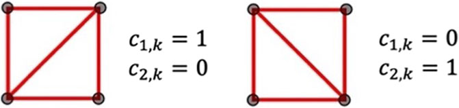
FIGURE 1. Bracing directions in the grid cell $k$ and corresponding values of $c_{1,k}$ and $c_{2,k}$

Since only one brace should exist in the grid cell $k$, the summation $c_{1,k}+c_{2,k}$ is always 1. Let ${\mathbf{c}}_1\in {\mathrm{ℝ}}^{n_{\text{x}}{n}_{\text{y}}}$ and ${\mathbf{c}}_2\in {\mathrm{ℝ}}^{n_{\text{x}}{n}_{\text{y}}}$, respectively, be vectors consisting of $c_{1,k}$ and $c_{2,k}$ for all bracing elements. The global stiffness matrix of the structure is a function of ${\mathbf{c}}_1$ and ${\mathbf{c}}_2$ denoted as $\mathbf{K}\left({\mathbf{c}}_1,{\mathbf{c}}_2\right)$. The bracing direction optimization problem to minimize the strain energy is formulated as follows:

$\text{minimize }E\left({\mathbf{c}}_1,{\mathbf{c}}_2\right)=\left(1/2\right)\cdot {\mathbf{d}}^{\text{T}}\mathbf{K}\left({\mathbf{c}}_1,{\mathbf{c}}_2\right)\mathbf{d}(\mathrm{3a})$

$\text{subject to }{c}_{1,k} , c_{2,k}\in \left\{\mathrm{0,1}\right\}, \left(k=1,2,\dots ,n_{\text{x}}{n}_{\text{y}}\right)(\mathrm{3b})$

$c_{1,k}+ c_{2,k}=1, \left(k=1,2,\dots ,n_{\text{x}}{n}_{\text{y}}\right)(\mathrm{3c})$

where $\mathbf{d}$ is an implicit function of ${\mathbf{c}}_1$ and ${\mathbf{c}}_2$ obtained by solving Eq. 1.

3 Graph Convolutional Network

Consider a graph consisting of $n$ nodes with $g$ features in each node. The graph data can be represented using a node feature matrix $\mathbf{N}\in {\mathrm{ℝ}}^{n\times g}$ representing features of each node in the graph, an adjacency matrix $\mathbf{M}\in {\mathrm{ℝ}}^{n\times n}$ representing the connectivity of structural elements, a weighted adjacency matrix $\mathbf{P}\in {\mathrm{ℝ}}^{n\times n}$ representing the connectivity of structural elements weighted by element forces, and a degree matrix $\mathbf{D}\in {\mathrm{ℝ}}^{n\times n}$ representing the number of connections of each node in the graph. Kipf and Welling (Kipf and Welling, 2017) proposed a GCN that can process graph input data which are chosen from $\left\{\mathbf{N},\mathbf{M},\mathbf{P},\mathbf{D}\right\}$, and map the inputs to the target domain of the graph for tasks such as node classification or link (connection) prediction (i.e., perform supervise learning by comparing mapped target domain from GCN to the node classification training data). A single GCN computation can be considered as a layer. Multiple GCN layers can be connected together to create a computational model for an RL agent. A GCN layer consists of a normalized form of adjacency matrix $\tilde{\mathbf{M}}$, and converts the input instances $\mathbf{N}$ to the output $\mathbf{O}\in {\mathrm{ℝ}}^{n\times h}$ that has $h$ embedding spaces (i.e., output for the GCN or output for a GCN layer that will be treated as $\mathbf{N}$ for the next GCN layer). The GCN layer can be formulated as follows:

$\mathbf{O}=\text{σ}\left(\tilde{\mathbf{M}}\mathbf{Nw}\right)(4)$

where $\text{σ}$ is a non-linear activation function, and $\mathbf{w}\in {\mathrm{ℝ}}^{g\times h}$ is the weight matrix (i.e., the convolution filter parameters) (Kipf and Welling, 2017) in the GCN layer which is adjusted during the training. The convolutional filter parameters $\mathbf{w}$ weight $\tilde{\mathbf{M}}\mathbf{N}$, an aggregated signal of a node and its neighboring nodes. It should be noted that $\mathbf{w}$ can handle any graph with any number of nodes as long as the nodes have the same number of features.

The normalized adjacency matrix $\tilde{\mathbf{M}}$ can be computed using the following equation:

$\tilde{\mathbf{M}}={\mathbf{D}}^{-1/2}\left[\mathbf{M}+\mathbf{I}\right]{\mathbf{D}}^{-1/2}(5)$

where $\mathbf{I}\in {\mathrm{ℝ}}^{n\times n}$ is the identity matrix, and ${\mathbf{D}}^{-1/2}$ is the inverse of the matrix ${\mathbf{D}}^{1/2}$ satisfying. ${\mathbf{D}}^{1/2}{\mathbf{D}}^{1/2}=\mathbf{D}$

In this paper, we utilize GCN to build an RL agent. The original GCN does not utilize the weighted adjacency matrix. However, for the structural optimization problem, the internal forces (i.e., the forces taken by the structural elements) should be utilized to guide the actions of the RL agent. Therefore, we propose a novel GCN-DDPG architecture that employs weighted adjacency matrices constructed from the internal forces for solving the bracing direction optimization problem. Details of the formulation are given in Section 5.

4 Reinforcement learning and Deep Deterministic Policy Gradient

RL is a type of ML that trains an agent to perform actions in an environment using reward signals. An RL algorithm consists of three main elements: a policy that determines the agent behavior, a reward signal that defines how good/bad the agent behavior is, according to the policy, and a value function that predicts how the agent performs based on the policy (Sutton and Andrew, 2018). The interaction of an agent and the environment is formulated using a Markov Decision Process (MDP) (Bellman, 1954; Bellman, 1957) as follows:

In a discrete step $t$:

The agent receives a representation of the environment as state ${\text{S}}_t$.

The agent performs actions ${\text{A}}_t$.

The agent receives quantitative reward ${\text{R}}_{t+1}$ and next state ${\text{S}}_{t+1}$ from the environment.

The diagram of the MDP can be represented as shown in Figure 2.

FIGURE 2

FIGURE 2. Diagram of the MDP

DDPG (Lillicrap et al., 2016) is a type of RL policy gradient algorithm that utilizes a parameterized policy function (Actor) ${\mathbf{\pi }}_{{{\displaystyle \text{θ}}}_1}$ to determine the probability of taking action ${\text{A}}_t^i$ in a state ${\text{S}}_t$, denoted by $\text{P}\left({\text{A}}_t^i\right|{\text{S}}_t)$, and another parameterized value function ${\text{Q}}_{{{\displaystyle \text{θ}}}_2}$ (Critic) to predict the accumulated reward (Q-Value) from the actions of the agent follows:

${\mathbf{\pi }}_{{{\displaystyle \text{θ}}}_1}\left({\text{S}}_t\right)=\text{ P}\left({\text{A}}_t^i|{\text{S}}_t\right)(6)$

${\text{Q}}_{{{\displaystyle \text{θ}}}_2}\left({\text{S}}_t,{\mathbf{\pi }}_{{{\displaystyle \text{θ}}}_1}\left({\text{S}}_t\right)\right)={\displaystyle \sum _{v=1}^{\infty }{\text{γ}}^{v-1}{\text{R}}_{t+v} }(7)$

where ${\text{θ}}_1$ and ${\text{θ}}_2$ are parameters of policy and value functions to be adjusted during the training, respectively. $\text{γ}\in \left[\mathrm{0,1}\right)$ is a discount factor for the reward.

During training, the value function adjusts its parameter ${\text{θ}}_2$ to increase the accuracy of its prediction of accumulated reward using a replay buffer that stores data of $\left\{{\text{S}}_t,{\text{A}}_t,{\text{R}}_{t+1},{\text{S}}_{t+1}\right\}$, whereas the policy function adjusts its parameter ${\text{θ}}_1$ to increase the value predicted by the value function, which is equivalent to the obtained rewards, using the gradient $\nabla {\text{J}}_{{\text{θ}}_1}$ as described in the following DDPG algorithm. Since using the online policy and value functions will make the learning unstable, Haarnoja et al. (Haarnoja et al., 2018) proposed a tau update method that trains a surrogate policy function ${\mathbf{\pi }}_{{\text{θ}}_{\mathrm{1}}^{\prime }}^{\prime }$ and a surrogate value function ${\mathbf{Q}}_{{\text{θ}}_{\mathrm{2}}^{\prime }}^{\prime }$, and then gradually updates the parameters of these functions into the online functions using a small value of $\tau$ $\left(\tau \ll 1\right)$ at every tau update interval. Note that the agent interacts with the environment to collect data for the replay buffer using the online policy function.

Let $\mathrm{ℒ}\left(y,\widehat{y}\right)$ be a loss function between $y$ which represents the correct value of training data and a predicted value $\widehat{y}$. The training algorithm of DDPG is as follows:

DDPG algorithm:

1. Sample u training data $\left\{{\text{S}}_t,{\text{A}}_t,{\text{R}}_{t+1},{\text{S}}_{t+1}\right\}$ from the replay buffer and convert them into a set of vectors $\left\{{\mathbf{S}}_t,{\mathbf{A}}_t,{\mathbf{R}}_{t+1},{\mathbf{S}}_{t+1}\right\}$.

2. Update the parameters as follows:

 ${\mathbf{\pi }}_{{\text{θ}}_{\mathrm{1}}^{\prime }}^{\prime }\left({\mathbf{S}}_t\right)={\widehat{\mathbf{A}}}_t$ # Surrogate policy function ${\mathbf{\pi }}_{{\text{θ}}_{\mathrm{1}}^{\prime }}^{\prime }$ decides actions from ${\mathbf{S}}_t$

 ${\mathbf{\pi }}_{{\text{θ}}_1}\left({\mathbf{S}}_{t+1}\right)={\widehat{\mathbf{A}}}_{t+1}$ # Online policy function ${\mathbf{\pi }}_{{{\displaystyle \text{θ}}}_1}$ decides actions from ${\mathbf{S}}_{t+1}$

 ${\text{Q}}_{{\text{θ}}_{\mathrm{2}}^{\prime }}^{\prime }\left({\mathbf{S}}_t,{\mathbf{A}}_t\right)={\widehat{\mathbf{Q}}}_t$ # Surrogate value function ${\text{Q}}_{{\text{θ}}_{\mathrm{2}}^{\prime }}^{\prime }$ predicts reward from ${\mathbf{S}}_t$ , ${\mathbf{A}}_t$

 ${\text{Q}}_{{\text{θ}}_2}\left({\mathbf{S}}_{t+1},{\widehat{\mathbf{A}}}_{t+1}\right)={\mathbf{Q}}_{t+1}$ # Online value function ${\text{Q}}_{{{\displaystyle \text{θ}}}_2}$ predicts reward from ${\mathbf{S}}_{t+1}$ , ${\widehat{\mathbf{A}}}_{t+1}$

 $\mathrm{\nabla }{\text{Q}}_{{\text{θ}}_{\mathrm{2}}^{\prime }}^{\prime }={\mathrm{\nabla }}_{{\mathrm{\theta }}_{\mathrm{2}}^{\prime }}{\text{Q}}_{{\text{θ}}_{\mathrm{2}}^{\prime }}^{\prime }\left({\mathbf{S}}_t,{\mathbf{A}}_t\right){\mathrm{\nabla }}_{{\widehat{\mathbf{Q}}}_t}\mathrm{ ℒ}\left({\mathbf{R}}_{t+1}+{\mathbf{Q}}_{t+1},{\widehat{\mathbf{Q}}}_t\right)$ # Gradient of ${\text{Q}}_{{{\displaystyle \text{θ}}}_{\mathrm{2}}^{\prime }}^{\prime }$ to the loss function

 $\nabla {\text{J}}_{{\text{θ}}_{\mathrm{1}}^{\prime }}^{\prime }=-\mathrm{𝔼}\left[{\nabla }_{{\text{θ}}_{\mathrm{1}}^{\prime }}{\mathbf{\pi }}_{{\text{θ}}_{\mathrm{1}}^{\prime }}^{\prime }\left({\mathbf{S}}_t\right){\nabla }_{{\widehat{\mathbf{A}}}_t}{\text{Q}}_{{\text{θ}}_{\mathrm{2}}^{\prime }}^{\prime }\left({\mathbf{S}}_t,{\widehat{\mathbf{A}}}_t\right){|}_{{\widehat{\mathbf{A}}}_t={\mathbf{\pi }}_{{\text{θ}}_{\mathrm{1}}^{\prime }}^{\prime }\left({\mathbf{S}}_t\right)}\right]$ # Gradient of ${\mathbf{\pi }}_{{\mathrm{\theta }}_{\mathrm{1}}^{\prime }}^{\prime }$ to the Q-Value.

 Update ${\mathbf{\theta }}_2^{\prime }$ in ${\text{Q}}_{{\text{θ}}_2^{\prime }}^{\prime }$ using $\nabla {\text{Q}}_{{\text{θ}}_2^{\prime }}^{\prime }$

 Update ${\mathbf{\theta }}_1^{\prime }$ in ${\mathbf{\pi }}_{{\mathrm{\theta }}_{\mathrm{1}}^{\prime }}^{\prime }$ using $\nabla {\text{J}}_{{\mathrm{\theta }}_{\mathrm{1}}^{\prime }}^{\prime }$

 If tau update interval is reached:

  ${\mathbf{\theta }}_1=\left(1-\tau \right){\mathbf{\theta }}_1+\tau {\mathbf{\theta }}_1^{\prime }$ # Update parameters of ${\mathbf{\pi }}_{{{\displaystyle \text{θ}}}_1}$

  ${\mathbf{\theta }}_2=\left(1-\tau \right){\mathbf{\theta }}_2+\mathit{\tau }{\mathbf{\theta }}_2^{\prime }$ # Update parameters of ${\text{Q}}_{{{\displaystyle \mathrm{\theta }}}_2}$

In order to reduce training time of adjusting the weights in each layer of GCN using the gradients, optimizers such as stochastic gradient descent (SGD) (Robbins and Monro, 1951; Kiefer and Wolfowitz, 1952; Ruder, 2016) or Adam (Kingma and Ba, 2015), is used for updating ${\mathbf{\theta }}_1$ and ${\mathbf{\theta }}_2$. The exploration of DDPG’s policy is activated by adding small Ornstein-Uhlenbeck noise (Uhlenbeck and Ornstein, 1930) into the output value of the policy function.

5 Reinforcement learning for structural optimization

5.1 State

This research utilizes the graph representation to express structural data, such as nodal coordinates, boundary conditions, and internal forces, at each optimization step which is equivalent to a step $t$ in the MDP formulation.

Suppose we have five node features, and the $i$th row of the node feature matrix $\mathbf{N}\in {\mathrm{ℝ}}^{n\times 5}$ is represented as ${\mathit{n}}_{\mathit{i}}=\left\{\begin{array}{ccccc}{\mathit{x}}_i/\underset{p}{\max }{x}_p& y_{\mathit{i}}/\underset{p}{\max }{y}_p& z_i/z_{\text{max}}& {\mathit{k}}_{\text{free}}^i& {\mathit{k}}_{\text{fix}}^i\end{array}\right\}$, in which $x_i$, $y_i$, and $z_i$ are the coordinates of node $i$, $z_{\text{max}}$ is the pre-determined upper-bound value of $z_i$, $\underset{p}{\max }{x}_p$ and $\underset{p}{\max }{y}_p$ are the maximum coordinate values in each axis. Note that the minimum coordinate values are assumed to be 0 for all coordinates. $k_{\text{free}}^i$ and $k_{\text{fix}}^i$ are determined depending on the boundary condition. $\left(k_{\text{free}}^i,k_{\text{fix}}^i\right)=\left(0, 1\right)$ if node $i$ is fixed support, and $\left(k_{\text{free}}^i,k_{\text{fix}}^i\right)=\left(1, 0\right)$ if node $i$ is not supported.

In the adjacency matrix for frame elements ${\mathbf{M}}_1\in {\mathrm{ℝ}}^{n\times n}$, the existence of a frame element $e$ connecting nodes $i$ and $j$ is denoted as $m_{1ij}=m_{1ji}=k_{\text{frame}}^e$ where $m_{1_{ij}}$ indicates $(i,j)$ component of matrix ${\mathbf{M}}_1$. $k_{\text{frame}}^e$ indicates the existence and non-existence of a 12-DoFs frame element $e$ that connects nodes $i$ and $j$ by $k_{\text{frame}}^e=1$ and $0$, respectively. In the adjacency matrix for truss elements ${\mathbf{M}}_2\in {\mathrm{ℝ}}^{n\times n}$, the existence of a truss element $e$ connecting nodes $i$ and $j$ is represented as $m_{2ij}=m_{2ji}=k_{\text{truss}}^e$. $k_{\text{truss}}^e$ indicates the existence and non-existence of a 6-DoFs truss element $e$ that connects nodes $i$ and $j$ by $k_{\text{truss}}^e$ $=1$ and $0$, respectively. The combined adjacency matrix for frame and truss elements ${\mathbf{M}}_3\in {\mathrm{ℝ}}^{n\times n}$ is obtained by ${\mathbf{M}}_3={\mathbf{M}}_1+{\mathbf{M}}_2$.

In order to evaluate the efficiency of the structural configuration, this paper proposes weighted adjacency matrices to represent the element internal forces. For the frame element, only a single weighted adjacency matrix ${\mathbf{P}}_1\in {\mathrm{ℝ}}^{n\times n}$ is determined using the ratio between the bending moment and the axial force, which for this type of structure is a useful index that helps minimizing the strain energy. Suppose frame element $e$ connects nodes $i$ and $j$, the entry $p_{1ij}$ in ${\mathbf{P}}_1$ is determined as follows:

$p_{{{\displaystyle 1}}_{ij}}=k_{\text{frame}}^e{b}_{ei}^{\prime }/\left(a_e^{\prime }+1\right)(\mathrm{8a})$

$b_{ei}^{\prime }=\left(\left|b_{ei}\right|-b_{\text{f}}^{\text{max}}\right)/\left(b_{\text{f}}^{\text{max}}-b_{\text{f}}^{\text{min}}\right)(\mathrm{8b})$

$a_e^{\prime }=\left(\left|a_e\right|-a_{\text{f}}^{\text{max}}\right)/\left(a_{\text{f}}^{\text{max}}-a_{\text{f}}^{\text{min}}\right)(\mathrm{8c})$

where $b_{ei}$ is the bending moment around the horizontal axis on the section at node $i$, and $a_e$ is the axial force of frame element $e$. $b_{\text{f}}^{\text{max}}$ and $b_{\text{f}}^{\text{min}}$ are the maximum and minimum absolute values of bending moments at the element ends. $a_{\text{f}}^{\text{max}}$ and $a_{\text{f}}^{\text{min}}$ are the maximum and minimum absolute axial forces of frame elements. For the truss elements, weighted adjacency matrix $\left({\mathbf{P}}_2\in {\mathrm{ℝ}}^{n\times n}\right)$ is a normalized form of the truss axial force. The entry $p_{{{\displaystyle 2}}_{ij}}$ in ${\mathbf{P}}_2$ corresponding to element $e$ connecting nodes $i$ and $j$ is determined as follows:

$p_{{{\displaystyle 2}}_{ij}}=k_{\text{truss}}^e{a}_e^{\prime }(\mathrm{9a})$

$a_e^{\prime }=\left(\left|a_e\right|-a_{\text{q}}^{\text{max}}\right)/\left(a_{\text{q}}^{\text{max}}-a_{\text{q}}^{\text{min}}\right)(\mathrm{9b})$

where $a_e$ is the axial force in the truss element $e$. $a_{\text{q}}^{\text{max}}$ and $a_{\text{q}}^{\text{min}}$ are the maximum and minimum absolute values of axial forces for truss elements, respectively. All values in these weighted adjacency matrices are in the range of $\left[\mathrm{0,1}\right]$, which helps avoiding numerical instabilities during training.

The degree matrices for frame, truss, and combined frame and truss elements are denoted by ${\mathbf{D}}_1\in {\mathrm{ℝ}}^{n\times n}$, ${\mathbf{D}}_2\in {\mathrm{ℝ}}^{n\times n}$, and ${\mathbf{D}}_3\in {\mathrm{ℝ}}^{n\times n}$, respectively. Entries in each degree matrix ${\mathbf{D}}_u$ $(u=1, 2, 3)$ are computed using the associated adjacency matrix ${\mathbf{M}}_u$ $\left(u=1, 2, 3\right)$ as $d_{{{\displaystyle \text{u}}}_{\mathit{ij}}}={\delta }_{ij}\times {\displaystyle \sum _{i=1}^n{m}_{{{\displaystyle \text{u}}}_{\mathit{ij}}}}$, where ${\delta }_{ij}$ is the Kronecker delta which is 0 if $i\ne j$ and 1 if $i=j$. The normalized adjacency matrices of frame, truss, and combined frame and truss elements are ${\tilde{\mathbf{M}}}_1\in {\mathrm{ℝ}}^{n\times n}$, ${\tilde{\mathbf{M}}}_2\in {\mathrm{ℝ}}^{n\times n}$, and ${\tilde{\mathbf{M}}}_3\in {\mathrm{ℝ}}^{n\times n}$, respectively, which are computed using Eq. 5. The GCN-DDPG agent for bracing direction optimization uses ${\tilde{\mathbf{M}}}_1$, ${\tilde{\mathbf{M}}}_2$, ${\tilde{\mathbf{M}}}_3$, ${\mathbf{P}}_1$, ${\mathbf{P}}_2$, ${\mathbf{M}}_2$, and $\mathbf{N}$ as a representation of the environment ${\text{S}}_t$ which will be further explained in Section 5.2.

5.2 GCN-DDPG agent

Policy and value functions (i.e., Actor and Critic networks of a GCN-DDPG agent) consist of multiple GCN layers. The policy function takes state data described in Section 5.1 as input to compute the output denoted as $\mathbf{O}\in {\mathrm{ℝ}}^{n\times h}$ which has the same number of rows as those of the node feature matrix $\mathbf{N}\in {\mathrm{ℝ}}^{n\times g}$. This output is used to determine bracing directions, explained in Section 5.3.

The inputs of the value function are state data and the output from the policy function to compute an estimation of the accumulated reward. In the value function, another matrix for prediction of the bracing directions denoted as ${\mathbf{M}}_{\text{o}}\in {\mathrm{ℝ}}^{n\times n}$ is internally computed from the output of the policy function $\mathbf{O}\in {\mathrm{ℝ}}^{n\times h}$, multiplied element-wise with ${\mathbf{M}}_2$ to exclude non-bracing elements, and normalized within the range [0,1] through dividing by $h$ as ${\mathbf{M}}_{\text{o}}=\left(\mathbf{O}\cdot {\mathbf{O}}^{\text{T}}\right)\odot {\mathbf{M}}_2/h$, where $\odot$ is the element-wise multiplication.

When multiple GCN layers are connected, a node feature matrix is replaced with an output from the prior GCN layer. To represent internal forces in the structure, a normalized adjacency matrix in a GCN layer can be replaced with a weighted adjacency matrix. The output of a GCN layer is transformed by the Rectified Linear Unit (ReLU) activation function (Nair and Hinton, 2010) similar to the original GCN (Kipf and Welling, 2017) for all layers of both policy and value functions. ReLU is a nearly linear function that is computationally efficient for gradient-based optimization (i.e., SGD or Adam) (Chigozie et al., 2020). ReLU is applied to all layers of both policy and value functions except the last layer of the policy function which is processed by the Sigmoid activation function for predicting probability-based output (i.e., probability of taking action ${\text{A}}_t^i$ in a state ${\text{S}}_t$) (Chigozie et al., 2020). Eq. 10a and Eq. 10b represent GCN layers with ReLU and Sigmoid activation functions, respectively, where ${\mathbf{N}}^{\prime }\in {\mathrm{ℝ}}^{n\times g}$ denotes a node feature matrix or an output from a prior GCN layer and ${\mathbf{M}}^{\prime }\in {\mathrm{ℝ}}^{n\times n}$ denotes ${\tilde{\mathbf{M}}}_1$, ${\tilde{\mathbf{M}}}_2$, ${\tilde{\mathbf{M}}}_3$, ${\mathbf{P}}_1$, ${\mathbf{P}}_2$, or ${\mathbf{M}}_{\text{o}}$ with size ${\mathrm{ℝ}}^{n\times n}$. Eq. 10c represents multiple computing loops using the same GCN layer.

$\text{μ}\left({\mathbf{N}}^{\prime },{\mathbf{M}}^{\prime }\right)=\text{ReLU}\left({\mathbf{N}}^{\prime }{\mathbf{M}}^{\prime }{\mathbf{w}}_{\text{μ}}\right)(\mathrm{10a})$

$\text{σ}\left({\mathbf{N}}^{\prime },{\mathbf{M}}^{\prime }\right)=\text{Sigmoid}\left({\mathbf{N}}^{\prime }{\mathbf{M}}^{\prime }{\mathbf{w}}_{\text{σ}}\right)(\mathrm{10b})$

${\text{iter}}^{\varphi }\left[\text{μ}\left({\mathbf{N}}^{\prime },{\mathbf{M}}^{\prime }\right)\right]=\underbrace{\text{μ}\left({\mathbf{M}}^{\prime }\left(\text{μ}\left({\mathbf{M}}^{\prime }(\dots ){\mathbf{w}}_{\text{μ}}\right)\right){\mathbf{w}}_{\text{μ}}\right)}\varphi \text{times}(\mathrm{10c})$

where $\text{ReLU}(\cdot )=\text{max}\left(0,\cdot \right)$, $\text{Sigmoid}(\cdot )=1/\left(1+{\text{e}}^{-(\cdot )}\right)$, and $\varphi$ in ${\text{iter}}^{\varphi }[ ]$ indicates the number of computing loops.

Since the output of a GCN layer is a matrix but the value function output is a scalar representing the estimation of accumulated reward, two operations are used for transforming the output matrix of the last GCN layer of the value function into a scalar value. The first operation is a global sum pooling operation (GSP) (Aich and Stavness, 2018) which transforms the output matrix into a vector by summing up all entries in each column of the output matrix. Let $\mathbf{V}\in {\mathrm{ℝ}}^{n\times g}$ be a matrix, the GSP operation to transform $\mathbf{V}$ into a vector can be represented as

$\text{Pool}\left(\mathbf{V}\right)=\left[\begin{array}{ccc}{\displaystyle \sum _{i=1}^n{\text{v}}_{i,1}}& \cdots & {\displaystyle \sum _{i=1}^n{\text{v}}_{i,g}}\end{array}\right]\in {\mathrm{ℝ}}^{1\times g}(11)$

The second operation is to compute the estimation of accumulated reward (i.e., Q-value $\in {\mathrm{ℝ}}^{1\times 1}$) from the vector output of the GSP operation using a neural network which consists of approximation functions that have adjustable weight parameters and activation functions (Goodfellow et al., 2016). These approximation functions are connected together so that the output of the prior approximation function is the input of the next approximation function, similarly to how the GCN layers are connected, where every approximation function, except the last one, is called a hidden layer (Goodfellow et al., 2016). Eq. 12 represents an NN with two hidden layers, used in this work, for computing the estimation of accumulated reward from the vector output of the GSP operation $\mathbf{H}\in {\mathrm{ℝ}}^{1\times g}$ with adjustable internal weight matrices ${\mathcal{W}}_1$, ${\mathcal{W}}_2$, ${\mathcal{W}}_{\text{out}}$, adjustable internal bias vectors ${\mathcal{B}}_1$ and ${\mathcal{B}}_2$, and adjustable internal bias scalar ${\mathcal{B}}_{\text{out}}$ as

${\text{f}}_{\text{NN}}\left(\mathbf{H}\right)={\mathcal{W}}_{\text{out}}{\left(\text{ReLU}\left({\mathcal{W}}_2{\left(\text{ReLU}({\mathcal{W}}_1{\mathbf{H}}^{\text{T}}+{\mathcal{B}}_1)\right)}^{\text{T}}+{\mathcal{B}}_2\right)\right)}^{\text{T}}+{\mathcal{B}}_{\text{out}}\in {\mathrm{ℝ}}^{1\times 1}(12)$

Table 1 summarizes the computation processes of the policy and value functions of the GCN-DDPG agent for bracing direction optimization. In each column, the 1st row indicates if the computation belongs to the policy or the value function. The 2nd row denotes input data used for the computation. The 3rd row indicates the computation process using GCN layers, GSP operation, and NN in Eqs 10a–12a–Eqs 10a–12.

TABLE 1

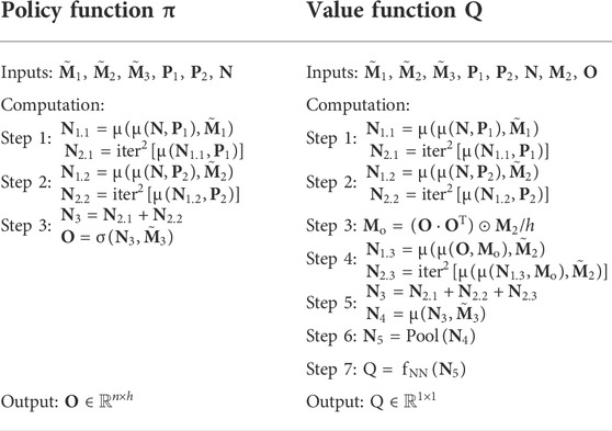
TABLE 1. Policy and value functions of GCN-DDPG for bracing direction optimization.

In the policy function, inputs from state data of frame and truss elements are separately processed in Steps 1 and 2, respectively. Output matrices in Steps 1 and 2 are combined to compute the output of the policy function in Step 3. In the value function, inputs from state data of frame and truss are also processed separately in Steps 1 and 2. Step3 computes the matrix for element direction prediction ${\mathbf{M}}_{\text{o}}$ which is used for processing action data in Step 4. Output matrices from the Steps 1, 2, and 4 are combined and re-processed by another GCN layer in Step 5. In Steps 6 and 7, the output matrix is converted into a vector using the GSP operation and the vector is finally converted to the Q-value by the NN. The last row denotes the output of the functions.

5.3 Action

The bracing direction in each grid cell is determined from a dot product of each row of $\mathbf{O}\in {\mathrm{ℝ}}^{n\times h}$ from the policy function output, similarly to the link prediction using GCN (Kipf and Welling, 2016) for the existence of a connection between two nodes in the graph. In this paper, the structural nodes are represented as graph nodes. Therefore, the prediction of a link or connection between two structural nodes is equivalent to a structural element (bracing element) that connects those nodes. Figure 3 shows a 4-node structure in a grid cell with two possible diagonal braces which connect node $i$ to node $j$ and node $n$ to node $m$, respectively. The dot product of each output matrix is used to predict the value of $l_{ij}$ and $l_{nm}$. $l_{ij}$ is equivalent to $l_{ji}$ and $l_{nm}$ is also equivalent to $l_{mn}$ as shown in the matrix in Figure 3. The bracing direction optimization formulation in Eqs 3a–ca–cEqs 3a–c allows only one brace in each grid cell. Therefore, $l_{ij}$ and $l_{nm}$ are compared to determine the bracing direction in a grid cell.

FIGURE 3

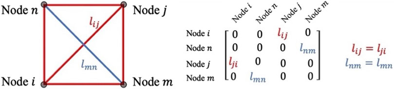
FIGURE 3. Bracing directions and associate link predictions in a grid cell.

The number of nodal embedding output dimensions is 100; i.e., $h=100$. From the output of the policy function $\mathbf{O}\in {\mathrm{ℝ}}^{n\times 100}$, the brace in grid cell $k$ is determined as

${\text{A}}_t^k=\{\begin{array}{cc}(c_{1,k}, c_{2,k})=(1, 0)& \left(\text{if }{l}_{ij}>l_{mn}\right)\\ (c_{1,k}, c_{2,k})=(0,1)& \left(\text{if }{l}_{ij}<l_{mn}\right)\end{array}(\mathrm{13a})$

$l_{ij} = l_{ji}={\displaystyle \sum _{u=1}^{100}{o}_{i,u}{o}_{j,u}}(\mathrm{13b})$

$l_{mn}=l_{nm}={\displaystyle \sum _{u=1}^{100}{o}_{n,u}{o}_{m,u}}(\mathrm{13c})$

At each step, the agent can change any number of brace directions.

5.4 Reward

In RL, a reward signal is used for training an agent. The reward signal ${\text{R}}_{t+1}$ that the agent receives after executing action ${\text{A}}_t$ in a state ${\text{S}}_t$ at step $t$ is formulated from the change of the strain energy as follows:

${\text{R}}_{t+1}=\left(E_t-E_{t+1}\right)/E_0(14)$

where $E_t$ and $E_0$ are the strain energy of the structure at step $t$ and the strain energy of the initial structure.

6 Numerical examples

6.1 General experiment setting and structural model

The agent is trained to optimize the structure in the training phase during which the ability to improve performance is assessed. In the test phase, the agent performance is evaluated on structural configurations other than those used in training. The method is implemented using Python 3.6 environment. A PC with CPU Intel Core i5-6600 (3.3 GHz, 4 cores) and GPU AMD Radeon R9 M395 2 GB is employed for computation.

Training is carried out on a grid shell structure with 4 × 4 grids and diagonal truss braces. Each grid cell has dimensions of 1.0 m by 1.0 m. To simplify the problem, the 12-DoFs frame element has a hollow cylindrical section with an external diameter of 100 mm and an internal diameter of 90 mm. The 6-DoFs truss element has a solid circular section with a diameter of 43.6 mm. Both elements have Young’s modulus of 205 kN/mm² and a similar weight of 12 kg/m. All structural nodes are subjected to a vertical point load of 10 kN.

Results obtained in the test phase using the proposed method are compared with those of the enumeration method (EM) and the genetic algorithm (GA); EM is used for the benchmark when it is feasible to compute all possible solutions, and GA is used for the benchmark when computing all possible solution is not feasible due to the large search space.

The algorithm flowcharts for training and test phases are given in Figure 4. During the optimization, each MDP is denoted as a step. The loop of MDPs or a game is terminated when the final step is reached.

FIGURE 4

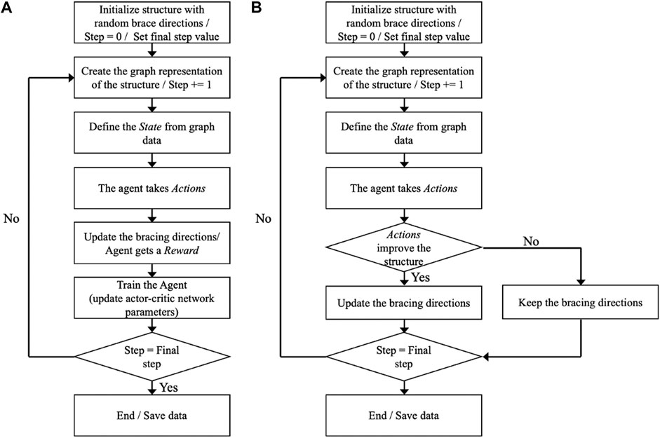
FIGURE 4. Algorithms of the proposed method; (A) Training phase, (B) Test phase.

6.2 Training phase

In each game of training, a dome-shaped structural model is initialized with supports assigned to two pre-determined structural shapes indicated in Figure 5. The maximum and minimum nodal height is 1 and 0 m, respectively. Note that structural shapes and size of structural elements are not adjusted during the optimization process. The brace directions are randomly initialized at every game.

FIGURE 5

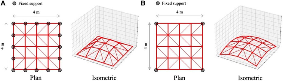
FIGURE 5. Structural models for bracing direction optimization during training phase; (A) Support condition 1, (B) Support condition 2.

The final step in each game is 200. At each step, the directions of braces are adjusted according to the agent actions. The agent surrogate functions are adjusted using the Adam optimizer. The mini-batch size is set to 32 and the learning rates are 10⁻⁷ and 10⁻⁶ for policy and value function, respectively. In the value function, the NN in Eq. 12 in Section 5.2 has two hidden layers, each consisting of 200 neurons. The mean square error is used as the loss function, and learning rates are reduced by a factor of $\beta$ = 0.1 every 200 games (20,000 steps). Weights and biases of the surrogate functions are synchronized with those of the online functions every 100 steps using $\tau$ = 0.05. The GCN-DDPG agent is trained for 1,000 games. In Figure 6, the vertical axis represents the cumulative reward obtained during training, and the horizontal axis is the game number. The thick line shows the moving average of the reward with a window size set to 50. From Figure 6, the cumulative reward increases during the first 200 games and then remains stable around a certain value. Because support and bracing directions are changed at every training game, the fact that the cumulative reward stabilizes indicates that the agent has the learning capability to optimize structural configurations of different topology and support conditions.

FIGURE 6

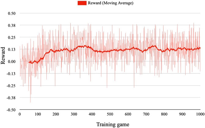
FIGURE 6. Variation of reward and its moving average in training phase.

6.3 Test phase

In the test phase, 4 × 4, 4 × 6, 6 × 6, 4 × 10, 10 × 6, 10 × 10, and 20 × 20-grid shells with pre-determined geometries are employed to investigate the capability of the trained agent on configurations that have not been tested in the training phase. In Figures 7–10, four support conditions denoted as 1, 2, 3, and 4 are considered for each frame model. The bracing directions are initialized randomly.

FIGURE 7

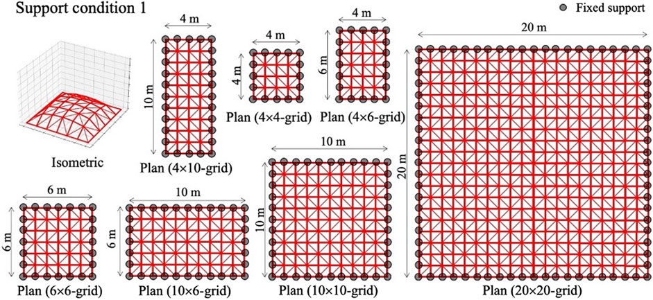
FIGURE 7. Structural models for test phase: Support condition 1.

FIGURE 8

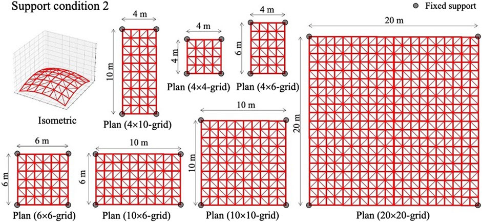
FIGURE 8. Structural models for test phase: Support condition 2.

FIGURE 9

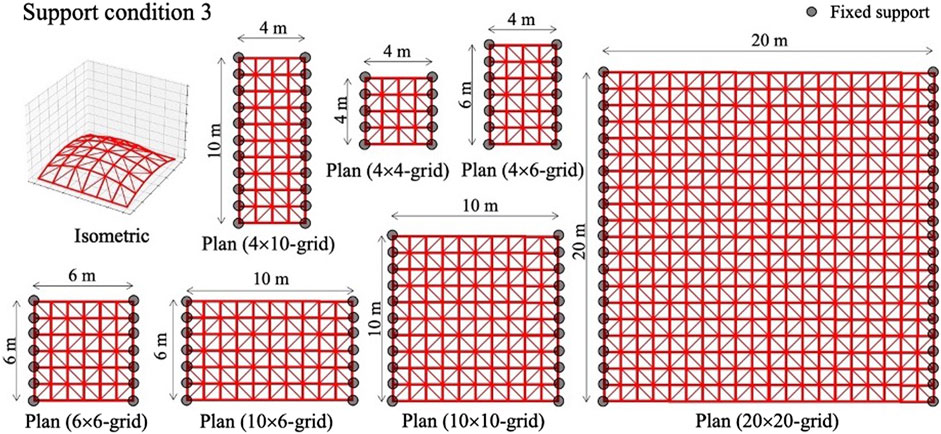
FIGURE 9. Structural models for test phase: Support condition 3.

FIGURE 10

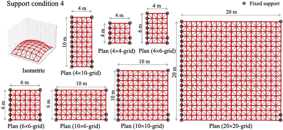
FIGURE 10. Structural models for test phase: Support condition 4.

Similarly to the training phase, the number of steps for the test phase is 100. However, in the test phase, only actions improving the objective function value are accepted at each step. The agent optimizes each structural model 10 times. Table 2 shows the minimum (Min.), mean, and standard deviation (Std.) for the strain energy, and mean energy reduction rate (Reduction) for each structural model.

TABLE 2

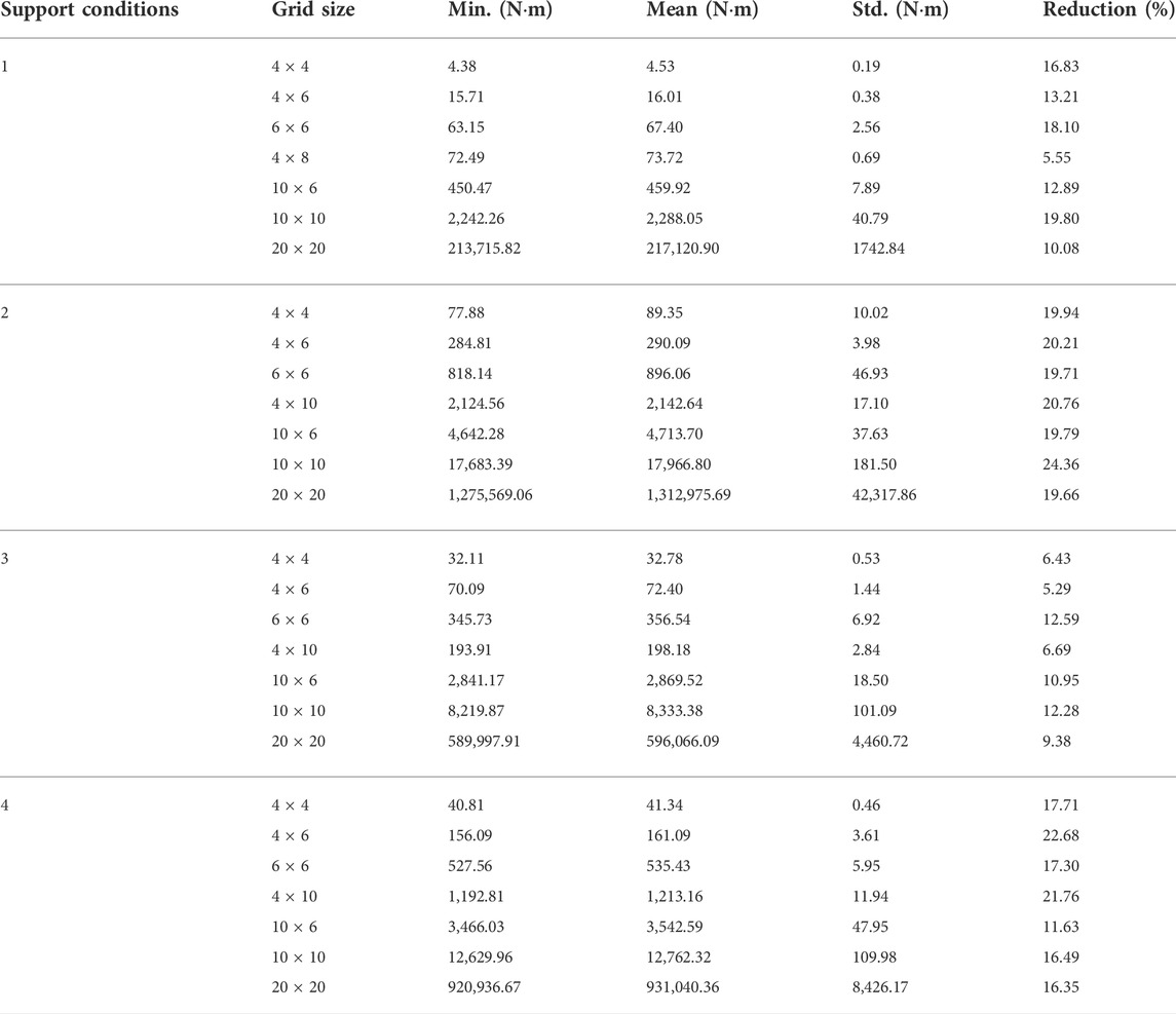
TABLE 2. Test results.

In the test phase, the strain energy of the structure can be reduced using the proposed method by 5–25%, depending on the structure size and support conditions. For all cases, the minimum and mean of strain energy obtained from 10 tests are very similar, and the standard deviations are low compared with the mean. The trained agent is capable to optimize the bracing directions to reduce the strain energy on configurations that were not tested in the training phase.

6.4 Comparison of computation cost and performance with EM and GA

For the 4×4-grid structure, the global optimal solution can be obtained using the EM which generates $2^k$ combinations of bracing directions for $k$ grid cells. For structures with a greater number of grids, it is not feasible to use EM. Therefore, the GA is employed to obtain optimal solutions (global optimum cannot be guaranteed). GA is a meta-heuristic method inspired by the process of natural evolution which can be used to solve combinatorial optimization problems. The key operations in GA are selection to transfers good solutions from one generation to the next generation, crossover to generate new solutions, and mutation to modify solutions with a certain probability, which can be helpful to avoid local minima. In this research, bracing directions in each grid cell are represented through binary strings and the GA algorithm is taken from the GA python library named Distributed Evolutionary Algorithms in Python (DEAP) (Fortin et al., 2012). The comparison is made to benchmark both the performance and computational efficiency of GCN-DDPG and GA for the early-stage design of grid shells where several configurations are to be evaluated. Therefore, the number of population and generation of GA are determined based on feasibility of computational cost. In the following examples, the numbers of population and generations are 50 and 100, respectively.

The number of structural analyses carried out with GCN-DDPG in the training phase is equal to the number of training games multiplied by the number of steps in each training game, which is 100,000. A trained agent can be used in the test phase and in other problems without re-training. The computational cost of GCN-DDPG in the test phase, EM, and GA for each problem, and the size of the global stiffness matrix are shown in Table 3 where the last row indicates the total computational cost. The total number of structural analyses required by GCN-DDPG is less than that required by GA. Since a significant computation time is required for the analysis of large-size structures, the GCN-DDPG is more efficient than the GA when applied to bracing direction optimization of grid shell structures that comprise many elements.

TABLE 3

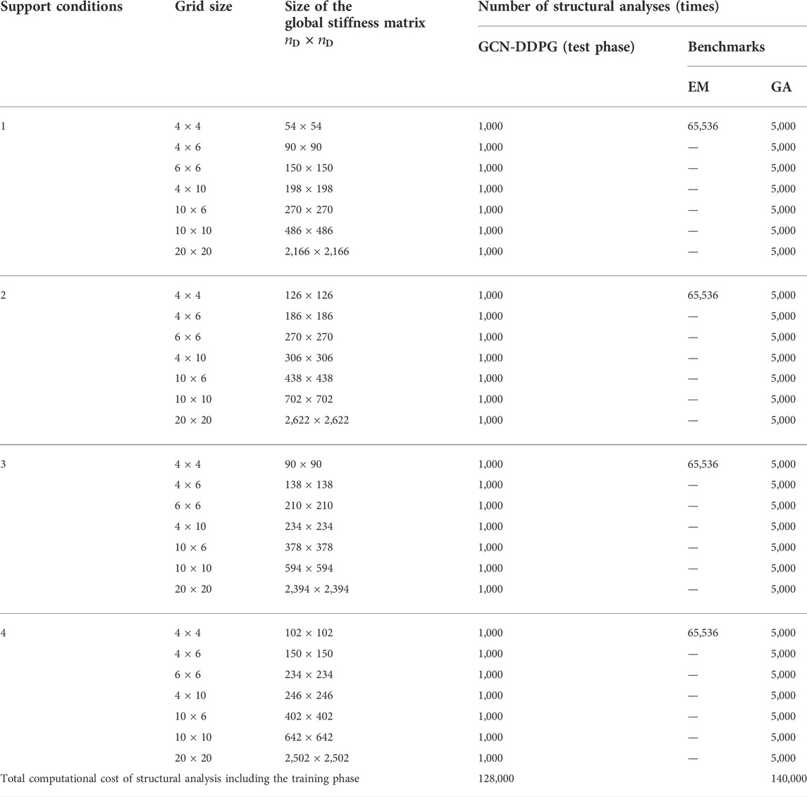
TABLE 3. Total computational cost of structural analysis of each method.

Benchmark results are compared in Table 4. The ratio of the difference between the minimum strain energy solution obtained by RL and that obtained by GA (and EM) is shown in the column labeled ‘Diff’, which is computed as follows:

$\text{Diff}=\left(\min \left({\text{Result}}_{\text{RL}}\right)-{\text{Result}}_{\text{GA}}\right)/{\text{Result}}_{\text{GA}}(15)$

TABLE 4

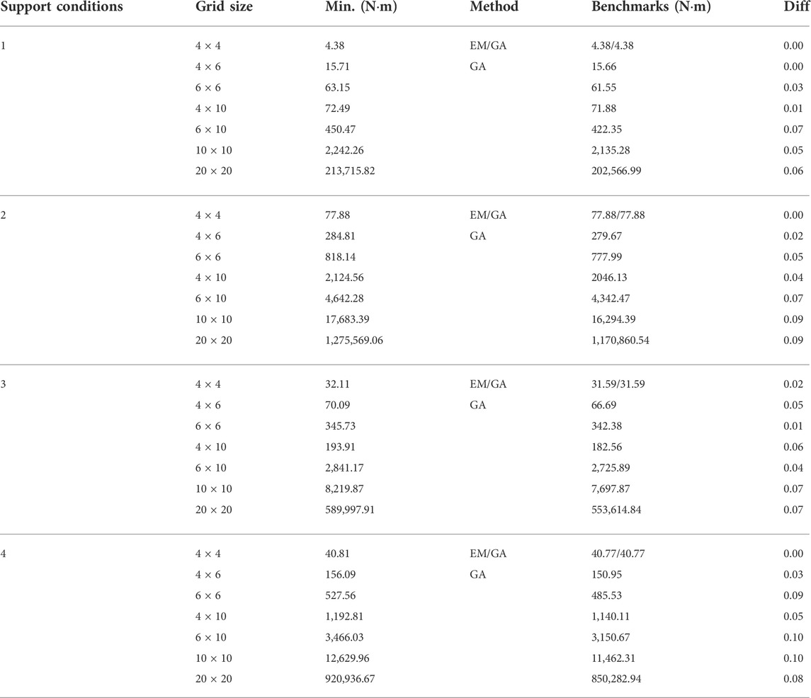
TABLE 4. Comparison of results obtained by GCN-DDPG (test phase) and benchmarks.

From Table 4, the solution quality and the efficiency of the GCN-DDPG agent can be verified. In most cases, results obtained by the GCN-DDPG agent are comparable to those obtained by EM and GA within a margin of 10% difference using less computational cost. The proposed method is useful in early-stage design, which typically requires testing several structures, and therefore an efficient computational process is needed. The RL agent could be further trained using other structural configurations to improve its performance.

Figure 11 shows initial brace topology, final brace topology, and the change of strain energy of GCN-DDPG best results for 6 × 6-grid structural models. Although the structural configurations differ considerably from those used in the training phase in terms of support conditions and size, the agent is capable to minimize the strain energy by adjusting the bracing directions. Therefore, it is possible to train the agent using small-size structural models and use it to optimize structures with different support conditions and sizes.

FIGURE 11

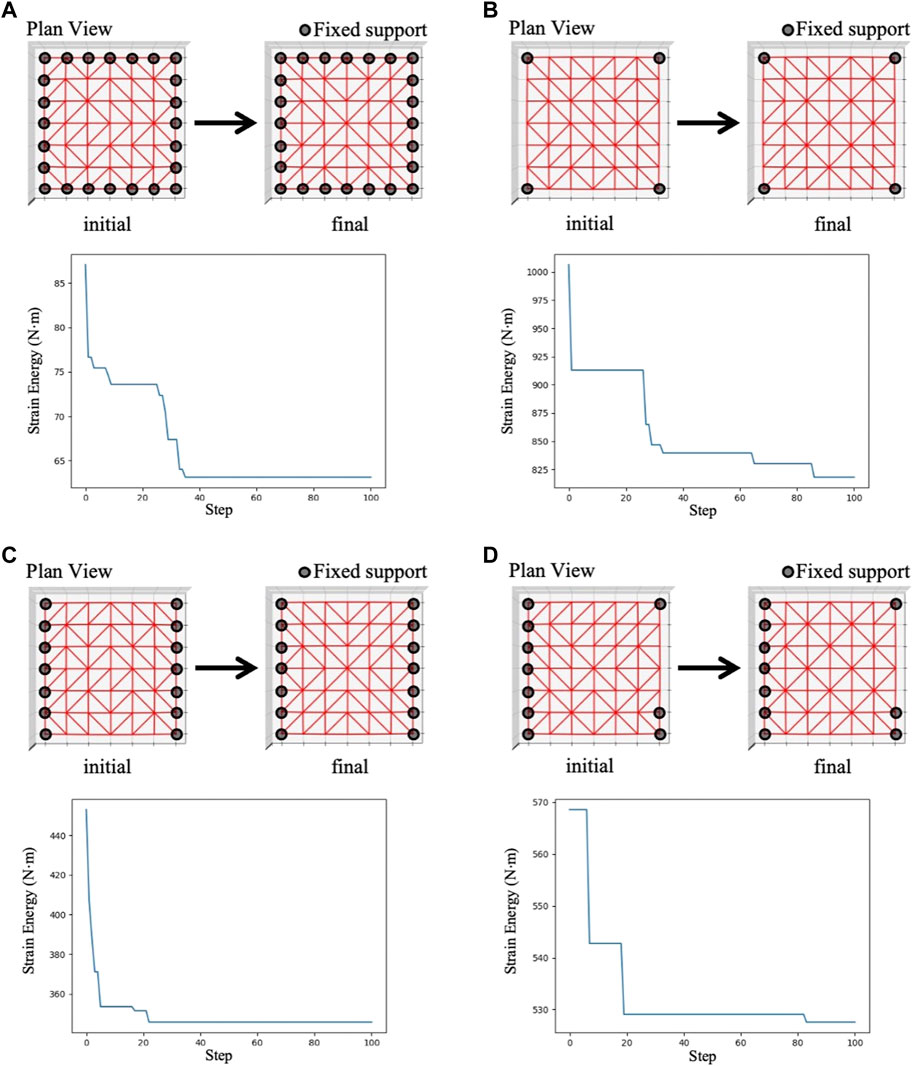
FIGURE 11. GCN-DDPG result of the 6×6-grid structure in the test phase; (A) Support condition 1, (B) Support condition 2, (C) Support condition 3, (D) Support condition 4.

From Figures 11A,C where the support locations are symmetric, the agent obtains solutions with symmetrical layouts, despite the fact that a symmetrical feature is not explicitly represented.

7 Conclusion

A combined method of DDPG and GCN has been formulated for bracing direction optimization of grid shell structures to minimize the strain energy. The proposed DDPG framework allows the agent to modify the bracing direction in all grid cells simultaneously at each optimization step. The node feature matrix, adjacency matrices, and weighted adjacency matrices are formulated to encode the structural configuration and internal forces as graph representations. The agent is trained using Markov Decision Process (MDP) in the RL framework whereby training data are collected by interacting with the environment. The value function or critic network updates internal weights and biases to minimize the prediction loss for the accumulated reward or Q-value so that it can predict the long-term accumulated reward from state and action. The policy function or actor network updates weights and biases to maximize the equivalent reward calculated by the value function.

Numerical examples show that the trained agent can effectively optimize bracing directions to minimize the strain energy in the test phase. The agent is capable to optimize the bracing direction of structural configurations with size and support conditions different than those in the training phase. The proposed method produces solutions that compare, albeit of marginally lower quality, with those produced through the enumeration method (EM) and the genetic algorithm (GA). However, the trained agent can be employed for additional configurations to those tested in this work. The agent performs well for relatively large structural models without the re-training, thereby significantly reducing the computational cost of optimization. Future work should investigate whether the RL method can be applied without re-training to design significantly larger-size structural configurations (e.g., 200 × 200 grid size) compared to those employed for training. Therefore, The proposed method has good potential to be employed effectively in early-stage design, which typically requires testing several configurations.

Data availability statement

Experiment data from this research are available on the request to corresponding authors.

Author contributions

C-tK: Conceptualization, implementation, writing-original draft, data curation. KH: Conceptualization, writing-review and editing, data curation, resource. MO: Conceptualization, writing-review and editing, data curation, resource.

Funding

This work was supported by MEXT scholarship (Grant Number 180136); and JSPS KAKENHI (Grant Numbers JP 20H04467, JP 21K20461).

Conflict of interest

The authors declare that the research was conducted in the absence of any commercial or financial relationships that could be construed as a potential conflict of interest.

Publisher’s note

All claims expressed in this article are solely those of the authors and do not necessarily represent those of their affiliated organizations, or those of the publisher, the editors and the reviewers. Any product that may be evaluated in this article, or claim that may be made by its manufacturer, is not guaranteed or endorsed by the publisher.

References

Aich, S., and Stavness, I. (2018). Global sum pooling: A generalization trick for object counting with small datasets of large images. Arxiv:1805.11123. [Online]. Available at: https://arxiv.org/abs/1805.11123.

Google Scholar

Bellman, R. (1954). The theory of dynamic programming. Bull. Amer. Math. Soc. 60 (6), 503–515. doi:10.1090/s0002-9904-1954-09848-8

CrossRef Full Text | Google Scholar

Bellman, R. (1957). A markovian decision process. Indiana Univ. Math. J. 6, 679–684. doi:10.1512/iumj.1957.6.56038

CrossRef Full Text | Google Scholar

Berke, L., and Hajela, P. (1993). “Application of neural nets in structural optimization,” in Optimization of large structural systems. NATO ASI series (Series E: Applied sciences). Editor G. I. N. Rozvany (Dordrecht: Springer), Vol. 231. doi:10.1007/978-94-010-9577-8_36

CrossRef Full Text | Google Scholar

Chigozie, N., Ijomah, W., Gachagan, A., and Stephen, M. (2020). Activation functions: Comparison of trends in practice and research for deep learning. Arxiv:1811.03378 [Online]. Available at: https://arxiv.org/abs/1811.03378.

Google Scholar

Christensen, P. W., and Klarbring, A. (2009). An introduction to structural optimization. Solid mechanics and its applications, Vol. 153. Dordrecht: Springer. doi:10.1007/978-1-4020-8666-3

CrossRef Full Text | Google Scholar

Dhingra, A. K., and Bennage, W. A. (1995). Topological optimization of truss structures using simulated annealing. Eng. Optim. 24 (4), 239–259. doi:10.1080/03052159508941192

CrossRef Full Text | Google Scholar

Eltouny, K., and Liang, X. (2021). Bayesian-optimized unsupervised learning approach for structural damage detection. Computer‐Aided. Civ. Infrastructure Eng. 36, 1249–1269. doi:10.1111/mice.12680

CrossRef Full Text | Google Scholar

Fortin, F. A., De Rainville, F. M., Gardner, M. A., Parizeau, M., and Gagné, C. (2012). DEAP: Evolutionary algorithms made easy. J. Mach. Learn. Res. Mach. Learn. Open Source Softw. 13, 2171–2175.

Google Scholar

Goodfellow, I., Bengio, Y., and Courville, A. (2016). Deep learning. The MIT Press. 9780262035613. Available at: https://www.deeplearningbook.org.

Google Scholar

Haarnoja, T., Zhou, A., Abbeel, P., and Levine, S. (2018). Soft actor-critic: off-policy maximum entropy deep reinforcement learning with a stochastic actor. ICML, 1856–1865. Arxiv:1801.01290. Available at: https://dblp.uni-trier.de/db/conf/icml/icml2018.html#HaarnojaZAL18.

Google Scholar

Hayashi, K., and Ohsaki, M. (2021). Reinforcement learning and graph embedding for binary truss topology Optimization under Stress and Displacement Constraints. Front. Built Environ. 6, 59. doi:10.3389/fbuil.2020.00059

CrossRef Full Text | Google Scholar

Hung, T. V., Viet, V. Q., and Thuat, D. V. (2019). A deep learning-based procedure for estimation of ultimate load carrying of steel trusses using advanced analysis. J. Sci. Technol. Civ. Eng. (STCE) - HUCE 13 (3), 113–123. doi:10.31814/stce.nuce2019-13(3)-11

CrossRef Full Text | Google Scholar

Ivakhnenko, A. G. (1968). The group method of data handling – a rival of the of stochastic approximation. Sov. Autom. Control 13 (3), 43–55.

Google Scholar

Jeong, M. J., and Yoshimura, S. (2002). “An evolutionary clustering approach to pareto solutions in multiobjective optimization,” in Proceedings of the ASME 2002 International Design Engineering Technical Conferences and Computers and Information in Engineering Conference, 141–148. doi:10.1115/DETC2002/DAC-34048

CrossRef Full Text | Google Scholar

Kanno, Y., and Fujita, S. (2018). Alternating direction method of multipliers for truss topology optimization with limited number of nodes: a cardinality-constrained second-order cone programming approach. Optim. Eng. 19 (2), 327–358. doi:10.1007/s11081-017-9372-3

CrossRef Full Text | Google Scholar

Kawamura, H., Ohmori, H., and Kito, N. (2002). Truss topology optimization by a modified genetic algorithm. Struct. Multidiscipl. Optim. 23, 467–473. doi:10.1007/s00158-002-0208-0

CrossRef Full Text | Google Scholar

Kiefer, J., and Wolfowitz, J. (1952). Stochastic estimation of the maximum of a regression function. Ann. Math. Stat. 23 (3), 462–466. doi:10.1214/aoms/1177729392

CrossRef Full Text | Google Scholar

Kingma, D., and Ba, J. (2015). “Adam: a method for stochastic optimization,” in 2014, Published as a conference paper at the 3rd International Conference for Learning Representations (San Diego). Arxiv:1412.6980.

Google Scholar

Kipf, T. N., and Welling, M. (2016). Variational graph auto-encoders. Arxiv:1611.07308. Available at: https://arxiv.org/abs/1611.07308.

Google Scholar

Kipf, T. N., and Welling, M. (2017). “Semi-supervised classification with graph convolutional networks,” in Proceedings of the 5th international conference on learning representations. Arxiv:1609.02907.

Google Scholar

Kociecki, M., and Adeli, H. (2015). Shape optimization of free-form steel space-frame roof structures with complex geometries using evolutionary computing. Eng. Appl. Artif. Intell. 38, 168–182. ISSN 0952-1976. doi:10.1016/j.engappai.2014.10.012

CrossRef Full Text | Google Scholar

Kupwiwat, C., and Yamamoto, K. (2020). Fundamental study on morphogenesis of shell structure using reinforcement learning. Struct. I 2020, 933–934. Architectural Institute of Japan. Available at: https://ci.nii.ac.jp/naid/200000462858/en/(Access March 17, 2022).

Google Scholar

Lillicrap, T. P., Hunt, J. J., Pritzel, A., Heess, N., Erez, T., Tassa, Y., et al. (2016). Continuous control with deep reinforcement learning, ICLR. Arxiv:1509.02971.

Google Scholar

MacQueen, J. (1967). “Some methods for classification and analysis of multivariate observations,” in 5-th Berkeley Symposium on Mathematical Statistics and Probability, 281–297.

Google Scholar

Mai, T. H., Kang, J., and Lee, J. (2021). A machine learning-based surrogate model for optimization of truss structures with geometrically nonlinear behavior. Finite Elem. Analysis Des. 196, 103572. ISSN 0168-874X. doi:10.1016/j.finel.2021.103572

CrossRef Full Text | Google Scholar

Mnih, V., Kavukcuoglu, K., Silver, D., Graves, A., Antonoglou, I., Wierstra, D., et al. (2013). Playing Atari with deep reinforcement learning. Arxiv:1312.5602. Available at: https://arxiv.org/abs/1312.5602.

Google Scholar

Nair, V., and Hinton, G. E. (2010). Rectified linear units improve restricted boltzmann machines. Haifa, 807–814. Available at: https://dl.acm.org/citation.cfm.

Google Scholar

Ohsaki, M., and Swan, C. (2002). “Topology and geometry optimization of trusses and frames,” in Recent advances in optimal structural design.

Google Scholar

Ohsaki, M. (1995). Genetic algorithm for topology optimization of trusses. Comput. Struct. 57 (2), 219–225. ISSN 0045-7949. doi:10.1016/0045-7949(94)00617-C

CrossRef Full Text | Google Scholar

Ohsaki, M. (2010). Optimization of finite dimensional structures. 1st ed.. Boca Raton, FL: CRC Press. doi:10.1201/EBK1439820032

CrossRef Full Text | Google Scholar

Puentes, L., Cagan, J., and McComb, C. (2021). Data-driven heuristic induction from human design behavior. J. Comput. Inf. Sci. Eng. 21 (2). doi:10.1115/1.4048425

CrossRef Full Text | Google Scholar

Robbins, H., and Monro, S. (1951). A stochastic approximation method. Ann. Math. Stat. 22 (3), 400–407. doi:10.1214/aoms/1177729586

CrossRef Full Text | Google Scholar

Rosenblatt, F. (1958). The perceptron: a probabilistic model for information storage and organization in the brain. Psychol. Rev. 65 (6), 386–408. doi:10.1037/h0042519

PubMed Abstract | CrossRef Full Text | Google Scholar

Ruder, S. (2016). An overview of gradient descent optimization algorithms. Arxiv:1609.04747. Available at: https://arxiv.org/abs/1609.04747.

Google Scholar

Sutton, R. S., and Andrew, G. B. (2018). Reinforcement learning, an introduction. 2nd ed. Cambridge, MA: The MIT Press. 9780262039246.

Google Scholar

Topping, B. H. (1983). Shape optimization of skeletal structures: A review. J. Struct. Eng. (N. Y. N. Y). 109, 1933–1951. doi:10.1061/(asce)0733-9445(1983)109:8(1933)

CrossRef Full Text | Google Scholar

Uhlenbeck, G. E., and Ornstein, S. L. (1930). On the theory of the Brownian motion. Phys. Rev. 36 (5), 823–841. doi:10.1103/PhysRev.36.823

CrossRef Full Text | Google Scholar

van der Maaten, L., and Hinton, G. (2008). Visualizing data using t-SNE. J. Mach. Learn. Res. 9, 2579–2605. Available at: http://jmlr.org/papers/v9/vandermaaten08a.html (Access March 17, 2022).

Google Scholar

Wang, D., Zhang, W. H., and Jiang, J. S. (2002). Truss shape optimization with multiple displacement constraints. Comput. Methods Appl. Mech. Eng. 191 (33), 3597–3612. ISSN 0045-7825. doi:10.1016/S0045-7825(02)00297-9

CrossRef Full Text | Google Scholar

Yu, A., Palefsky-Smith, R., and Bedi, R. (2019). Deep reinforcement learning for simulated autonomous vehicle control. Stanford, CA, USA: Stanford University. Available at: http://vision.stanford.edu/teaching/cs231n/reports/2016/pdfs/112_Report.pdf (Access March 17, 2022).

Google Scholar

Zhu, S., Ohsaki, M., Hayashi, K., and Guo, X. (2021). Machine-specified ground structures for topology optimization of binary trusses using graph embedding policy network. Adv. Eng. Softw. 159, 103032. ISSN 0965-9978. doi:10.1016/j.advengsoft.2021.103032

CrossRef Full Text | Google Scholar