 Yoshihiro Mogi
 Naohiro Nakamura
 Kunihiko Nabeshima1
 Akira Ota
94% of researchers rate our articles as excellent or good
Learn more about the work of our research integrity team to safeguard the quality of each article we publish.
Find out more
ORIGINAL RESEARCH article
Front. Built Environ., 18 March 2022
Sec. Earthquake Engineering
Volume 8 - 2022 | https://doi.org/10.3389/fbuil.2022.858029
This study investigates the performance of several capped viscous damping models which give an upper limit to the initial-stiffness-proportional damping force. The comparing capped viscous damping models are the original and newly proposed one. The original capped damping model is expected to have a certain degree of frequency insensitiveness. However, unless the damping force reaches the capped value, the damping may be simply behaving as the initial-stiffness-proportional damping, also there is no clear physical basis for setting the capping value. Conversely, it is confirmed that the newly proposed damping model improves the original model problems faced with setting the capping value and frequency insensitiveness accuracy. In this study, the discussion is primarily focused on structural engineering using a 20-story fish bone model comprising a steel and reinforced concrete, but this argument can be applied to various engineering fields such as civil and mechanical engineering. Especially, this proposed model does not have mass term damping, it may be effective for a large nonlinear analysis such as sliding/uplifting and base-isolated structure.
The main factors that influence the damping energy of a building are due to material friction and contact between non-structural elements and this damping does not greatly depend on frequency (Lazan (1968))., i.e., this damping is considered to more appropriately represent reality than viscous damping in numerical simulation (Clough and Penzien (2003)). However, in time history analysis, this hysteresis of damping must be expressed as complex damping. Hence, stiffness-proportional damping and Rayleigh damping have long been used, even if it is difficult to use if the damping should be constant over a wide frequency band. To compensate for this, constant modal damping is often used, but it lacks practicality for large-scale analysis because of to the large computing load. In recent times, performance-based building design is being increasing employed, and it is inevitable to increase the scale of analysis models via a numerical simulation technology. Therefore, there is a need to develop an ideal damping model.
Building damping is affected by various factors such as location conditions and aging, and it is difficult to evaluate it quantitatively because of the large variation. However, the selection of the damping model has considerable influence on the seismic response analysis and incorporating such physical quantities into numerical simulation is an important engineering issue. Recent papers Huang et al. (2019), Nakamura (2019), Mogi et al. (2021), and Ota et al. (2021) have attempted to solve this problem, describing a viscous damping scheme that achieves frequency independent damping over a wide frequency range. Although these damping models are excellent in overcoming the problems of the existing viscous damping models, high-level computational algorithms must be incorporated. Therefore, this study focused on the capped viscous damping for developing a damping model that easily realizes frequency independence. The capped damping model that gives an upper limit to the initial-stiffness-proportional damping force is expected to have a certain degree of frequency insensitiveness. However, unless the damping force reaches the capped value, the damping may simply behave as the initial-stiffness-proportional damping, and there is no clear physical basis for setting the capping value.
For overcoming the aforementioned problems, this study proposes a novel damping model that can clarify the concept of setting a capping force. Then, the effectiveness of the proposed model is demonstrated by comparing it with the original capped viscous damping model and other conventional models. Ultimately, we must confirm the practicality of the proposed model through 3D analysis, but first we analyzed the basic characteristics of the proposed damping model using a simple 20-story fish bone model.
Rayleigh damping is often used owing to its ease of use. It is a classical damping model expressed by damping terms proportional to mass m and initial stiffness
Hence, if coefficients
Coefficients
These two algebraic equations can be solved to determine coefficients
The stiffness-proportional term
The damping force
Wilson and Penzien (1972) expresses the modal damping matrix
Where,
In addition, Luco and Lanzi (2019) reported that in modal damping, after the nonlinear element transition from the elastic state to plastic state, the degree of freedom without mass becomes an unintended velocity response because of numerical artifacts and the absence of damping terms. To avoid this problem, model damping can be improved by adding infinitesimal stiffness-proportional damping.
The capped viscous damping model is a damping model that can be applied to a complex vibration model with large nonlinear behavior; for example, it can be applied to the sliding or uplifting of a foundation. Although tangent Rayleigh damping is effective in such an analysis, there is concern that tangent Rayleigh damping has little physical basis for reducing the damping force and that damping is overestimated owing to the influence of the mass term. Hall (2006) discusses the increase in the ratio of damping force to spring strength using a 10-story lumped mass shear model as an example. In the elastic state, the ratio of the restoring force and damping force is kept constant, but after yielding, the restoring force is limited, whereas the damping force increases in proportion to the velocity. This is unnatural and cannot be explained as a real phenomenon. In the case of initial-stiffness-proportional damping, the restoring force
If the spring is elastic and oscillated in the first mode, the peak values of the restoring force and damping force will maintain a ratio of
Here,
In addition to the effect of suppressing an abnormal increase in the damping force after yielding, caped damping has the characteristic of causing a certain degree of frequency insensitiveness. The capping fraction
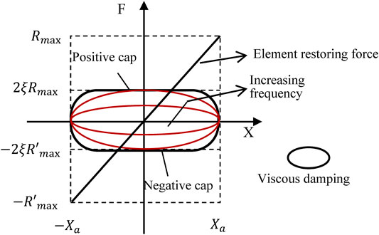
FIGURE 1. Element force and viscous damping forces vs. displacement for a single-degree-of-freedom oscillator under harmonic motion with increasing frequency at constant displacement amplitude X: Rmax is maximum restoring force of spring. [presented by Hall (2018)].
The limitations of the equivalent viscous damping model identified in previous studies are summarized as follows:
1) Generally, the viscous damping model depends on frequency (Clough and Penzien (2003)).
2) Using Rayleigh damping in inelastic RHA, a spurious damping force may be generated when stiff inelastic spring inserted at the beam-end is yielding (Chrisp (1980); Bernal (1994)).
3) The tangent Rayleigh damping concept is an ad hoc approach since there is no physical basis to such a damping mechanism (Hall (2006)).
4) Using Rayleigh or tangent Rayleigh damping in inelastic RHA, inappropriate damping forces are generated because of the changes in eigenmodes (Léger and Dussault (1992); Charney (2008)).
5) It is inappropriate to apply Rayleigh damping or constant modal damping to structures that are sliding/uplifting or to seismic base isolation structures owing to the influence of the mass term damping force (e.g., Hall (2006); Ryan and Polanco (2008); Pant and Wijeyewickrema (2012); Pant et al. (2013); Hamidreza et al. (2019)).
6) It is effective to use modal damping to avoid spurious damping force generation (Chopra and McKenna (2016)), but an unintended velocity response occurs with no mass degrees of freedom after the element transitions from elastic to inelastic (Luco and Lanzi (2019)).
7) The original capped viscous damping provides little rationale for setting the upper limit, and it is unclear how effective the capped damping force is on the frequency independence of stiffness-proportional damping. Furthermore, modeling by the story shear damping force is not enough when three-dimensional vibration is considered (Qian et al. (2021)).
In this study, we focused on the capped viscous damping proposed by Hall (2006) with the aim of exploring a well-balanced model that can avoid the aforementioned problems. The vibration characteristics were analyzed by comparing it with several damping models, and the engineering convenience/effectiveness of this damping model was considered.
The amount of capped damping force is an important factor for determining the damping characteristics. Hall (2006), Hall (2018), Qian et al. (2021) propose that the story shear damping force is capped at
If the building undergoes simple vibration in the first mode and the displacement is the maximum amplitude
Equation 9 shows that the damping force increases in proportion to
In the next section, we explain the setting of the maximum restoring force
This study proposes a capped damping force
1) If
2) If the restoring-force changes from the increasing state to the decreasing state,

FIGURE 2. Update procedure for the maximum amplitude of restoring force
The red and blue dashed lines in Figure 2 indicate the time domain in which
As described earlier, by setting the peak value of the most recently recorded restoring force to
Figure 3 shows the program flow which is written specifically test capped viscous damping. For the total equation of motion, incremental Eq. 10 at the integral time interval
FIGURE 3. Program flow.
Here,
The program performs the triangular decomposition of the effective stiffness matrix
The balance of the total equation of motion is calculated using the updated damping force vector
To evaluate the differences in the responses of different damping models, a comparative study was conducted using a fish bone model that simulates a high-rise building and a period for 2 s (Figure 4A). The vertical degrees of freedom of all nodes were constrained, and the horizontal displacement of the nodes at each beam level were equal to the that of the beam–column joint node by multi-point constraints. The story height was 3.5 m, and the span is assumed to be 6 m, and 3-m-long beams were set on the left and right. The beam and column sections are listed in Table 1. The beam stiffness was multiplied by Φ (=1.5) considering the slab, and the column stiffness was about 1.8–1.9 times that of the beam. A mass (59.19 t) was uniformly applied to each floor at the beam–column joint node as shown in Figure 4A so that the period was 2.0 s and the rotational inertia mass of each node was zero. To confirm the differences depending on the types of structures, two cases were considered: the case of the beam-end assuming a steel (S) structure with restoring-force characteristics is shown in Figure 4B, and the case of the beam-end assuming a reinforced concrete (RC) structure with the Takeda model is shown in Figure 4C. The initial stiffness and yield moment of the RC model are the same as those of the S model for convenience. The crack-bending strength of the Takeda model is assumed to be 0.3 times its yield strength, and the post-cracking stiffness is assumed to be 0.5 times the initial stiffness. Table 2 lists the initial stiffness (3EI/L) of the beam, post-cracking stiffness ratio, cracking moment, and yielding moment. The inelastic spring at the end of beam is generally incorporated into the element stiffness matrix implicitly or arranged explicitly with an additional node. In the arranged explicitly with an additional node case, the initial stiffness of the end hinge spring is set at a higher value so as that the linear natural vibration of the model is unaffected; however, the spurious damping force is prominent in such modeling (Chrisp (1980); Bernal (1994)). In this study, this method is used to insert an inelastic spring with stiffness 1,000 times higher than the beam (Figure 4D). Therefore, for the inelastic spring with nonlinear characteristics (Table 2), K1 should be multiplied by 1,000, and conversely, the post-cracking stiffness ratio of K2 and K3 should be multiplied by 1/1,000, and K2 gives 0.0005 and K3 gives 1.0E-6.
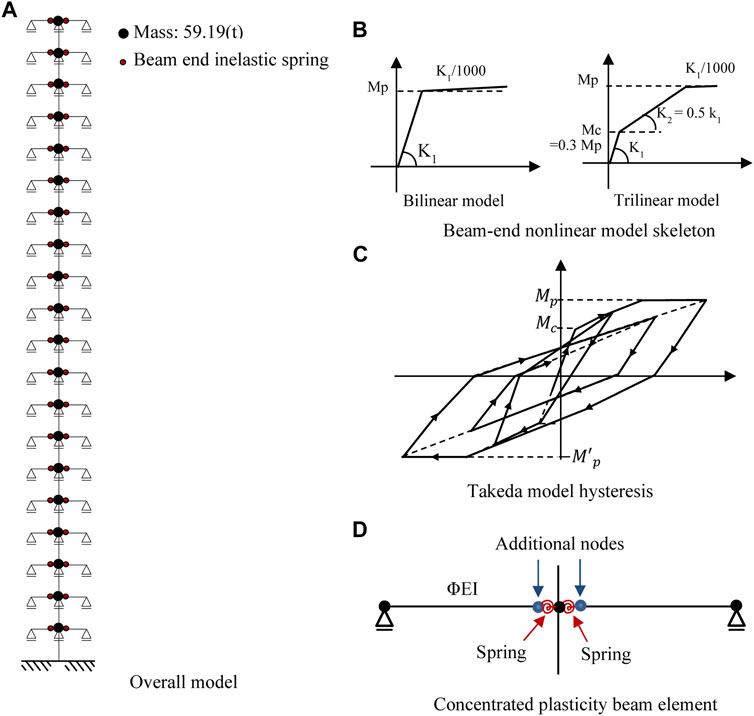
FIGURE 4. (A) Overall view of the 20-story fish bone model, (B) beam-end nonlinear model skeleton, (C) Takeda model hysteresis, and (D) concentrated plasticity beam element.
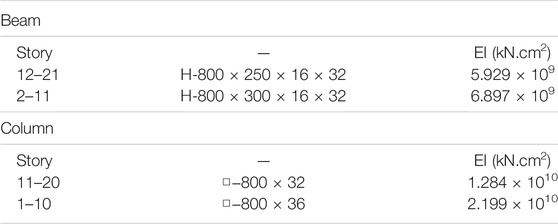
TABLE 1. Element stiffness.
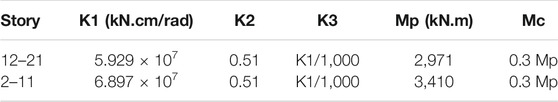
TABLE 2. Beam-end nonlinearity.
Table 3 lists the natural period and effective mass ratio (cumulative values from lower mode).
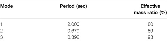
TABLE 3. Eigen value analysis results.
Ground motion was created by using an acceleration response spectrum with 5% damping as the target spectrum and using the random phase characteristic (return period of 500 years). Figure 5 shows the simulated ground motion and acceleration/pseudovelocity response spectra.
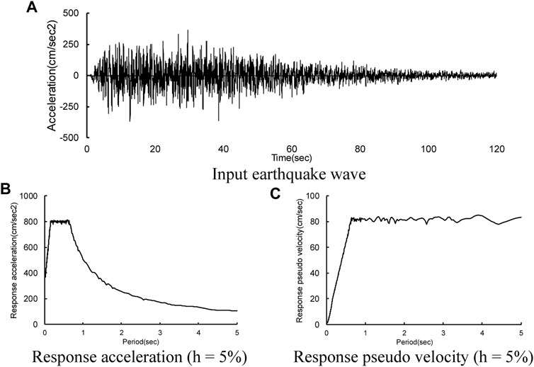
FIGURE 5. Simulated earthquake motion. (A) Input earthquake wave, (B) Response acceleration (h = 5%), (C) Response pseudo velocity (h = 5%).
The three types of capped viscous damping models, including the original capped viscous damping [CP(O)], capped viscous damping A [CP(A)], and capped viscous damping B [CP(B)] models, were compared to prove the effectiveness of the proposed modeling. The accuracy of each damping model was verified by comparison with the nonlinear constant modal damping model (WP), which creates a damping matrix by performing an eigenvalue analysis each time the structural stiffness changes.
The original or CP(O) model has been proposed as a method for giving a lateral interstory damper (Hall (2006); Hall (2018)). The same modeling was used in this study. The height-wise distribution of damper coefficients (
Where,

TABLE 4. Interstory capped damping force
The CP(A) is a method for determining the capped damping force. This was done by setting the maximum value of the restoring force experienced in the past as
The CP(B) was considered as the main method in this study. This is a method for determining the capped damping force from the maximum value of the most recently experienced restoring force, which was set as
The oscillation characteristic of constant modal damping WP, CP(A), and CP(B) were compared using three cycles of sinusoidal wave synchronized with the building period; further, CP(O) was not compared. The input wave is shown in Figure 6A. Using this input wave, the steady vibration at the time of input and the free vibration after the input can be examined in one analysis. The maximum acceleration was 100 gal, and the response analysis time was 30 s. The integration step was 0.001 s; the damping ratio was 2%; The responses obtained by using each sinusoidal wave tuned to the first mode to the third-mode periods of the frame were compared. Figure 6 shows the maximum story drift angle and acceleration for each floor. Figure 6B is the result of the first mode periodic input. The maximum responses of CP (A) and CP (B) consistently show the same results in the first to third modes. Further, CP(A) and CP(B) have slightly larger responses than WP. This is because as suggested in the previous section, the velocity precedes the displacement, and hence, the damping force peaked at the maximum value of the past restoration force, and the damping force could not be fully exerted. Moreover, as shown Figures 6C,D, the maximum response of the CP(A) and CP(B) of the second- and third-mode periodic inputs was the same as that of the WP. Figure 7 shows the mode RHA, which is the mode response
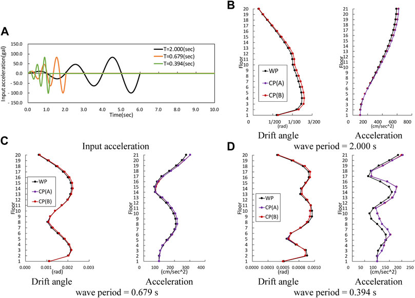
FIGURE 6. Maximum response for the sinusoidal wave. (A) Input acceleration, (B) wave period = 2.000 s, (C) wave period = 0.679 s, (D) wave period = 0.394 s.
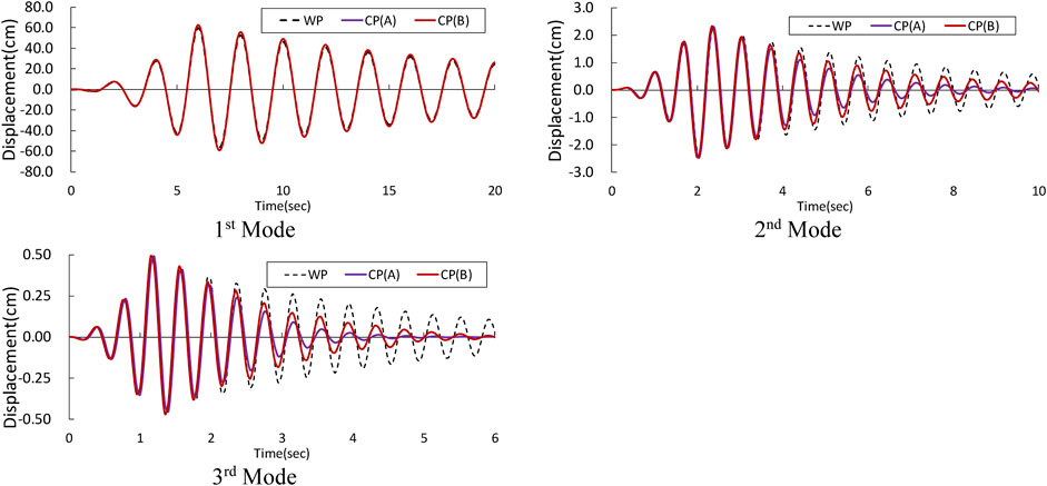
FIGURE 7. Modal displacement.
From Figure 7, we can see that the maximum response occurs at the final peak of the sweep excitation, but CP(A) and CP(B) show a relatively frequency insensitiveness characteristics for the response of such an amplification process. However, in the free vibration after the forced-excitation phase, there is a tendency to overestimate the damping slightly compared to the estimates of WP. This overestimation is attributed to the fact that since
Next, Evaluate the oscillation characteristics of real-phase seismic waves as elastic and inelastic. To compare the differences in the characteristics of the steel and reinforced concrete structures, the integration time step was 0.0001 s, and the damping ratio was 2% for both S and RC structures.
For the elastic RHA, according to the response results of the elastic analysis shown in Figure 8, the maximum interstory drift angles of the CP(B) and WP models are similar but that of CP(O) and CP(A) are smaller. The maximum displacement of the CP(O), CP(A), and WP models are similar but that of CP(B) is slightly larger. This tendency was also seen in the examination of sinusoidal waves, but it is attributed to the slight underestimation of the attenuation of the first mode. The maximum acceleration is observed for the WP model, followed by the CP(B), CP(A), and CP(O) models. Figure 9 shows the displacement time history response of each mode decomposed by the expansion theorem of shown in Eq. 18. Although the response of the all model is almost the same in the first mode, in higher mode, the responses of CP(O) and CP(A) are smaller than CP(B) and WP and the responses of CP(B) is slightly smaller than that of WP. However, in the third mode, the responses of all capped viscous damping models were smaller than that of the WP, and the higher mode tended to reduce the frequency insensitive effect of the damping force capping. From these results, the CP(B) shows relatively more frequency-insensitive characteristics than CP(O) and CP(A) in the elastic RHA.
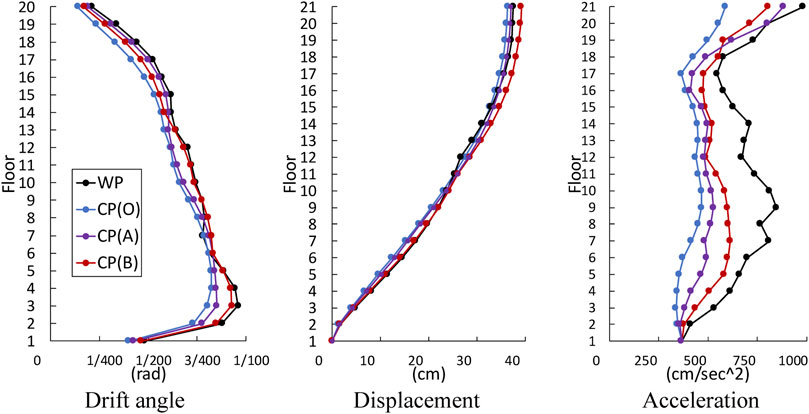
FIGURE 8. Maximum response of elastic response history analysis (RHA).
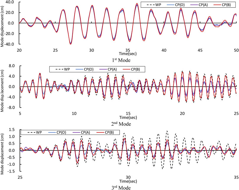
FIGURE 9. Time histories of the modal displacement.
Figure 10 shows the maximum responses obtained by inelastic analysis. The ductility factor was evaluated by the ratio of the maximum node rotation angle of the beam–column joint to the beam yield rotation angle. The RC ductility factor diagram also shows the ratio of the crack rotation angle to the yield rotation angle.
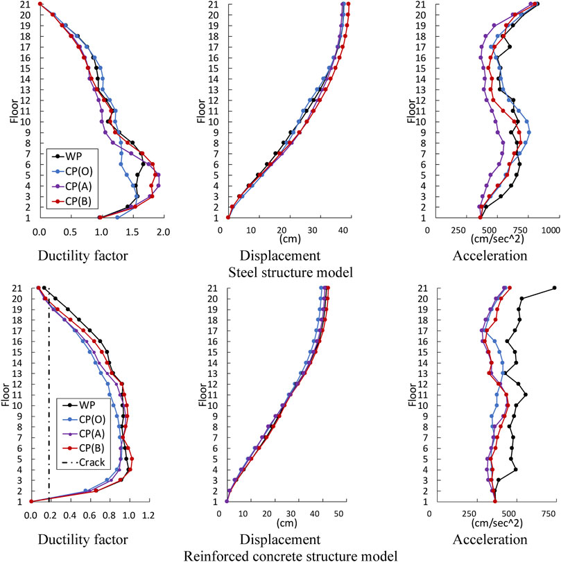
FIGURE 10. Maximum response of inelastic RHA.
In the steel structure model, the ductility factor, CP(A), and CP(B) correspond relatively well with the WP; however, its response was larger than the WP in the lower story. CP(O) also showed a relatively good response in the upper story; however, its response in the lower story was smaller than the other damping models. As for the displacement responses, CP(B) showed a slightly larger response than the other damping models. Meanwhile, the other models provided almost the same responses. In general, there were variations in the acceleration responses, where the CP(A) showed a smaller response than the other damping models.
In the RC structure model, the ductility factor and CP(O) showed smaller responses than the other damping models. Meanwhile, the other damping models gave almost the same responses. The displacement responses were almost the same in all the damping models. In general, the acceleration responses varied; however, the CP(O), CP(A), and CP(B) showed smaller responses than the WP.
These comparisons showed that the CP(B) varied in acceleration response from the WP. However, the displacement responses and ductility factors (story drift angles) were relatively in good agreement in both steel and RC structure models. The responses of the CP(O) were not as good.
From the above comparison, it is confirmed that CP(B) shows better characteristics than CP(O) and CP(A) in the inelastic RHA.
The proposed viscous damping force is estimated using the recently recorded maximum restoring force
This study assumes that the variable axial force due to horizontal movement does not act on the columns, but it is predicted that the large variable axial force due to the horizontal mode is applied to the corner columns or the side columns of the shear wall or brace. In this case, since the
Currently, the damping of vertical oscillation in buildings is not as clear as horizontal motion because the vertical motion is less than the horizontal motion and the destruction of the building is primarily caused by the horizontal motion. However, in structural design practice, evaluating the axial force ratio of columns, deformation due to beam vibration, and the surface pressure of seismic isolation bearings is essential. If vertical vibration mode is critical to structural design, its mechanism should not overestimate the damping force even when considering the simultaneity of multiple vibration modes. Because the capped viscous damping depends only on the stiffness term, the damping ratio of the element deformation component predicted to be over-damped is reduced in advance.
To verify the effectiveness of capped viscous damping based on the maximum restoring force experienced in the past, original method CP(O) and simple method CP(A) based on the past maximum value and a method CP(B) based on the latest maximum value were compared and verified. Capped viscous damping is a practical damping model with low computational load and no spurious damping force excitation. It is expected to be applied in the field of structural, civil and mechanical engineering. The findings of this study are as follows:
1) The original method has a problem in the capping force setting, and the appropriate value depends on the scale of the assumed seismic motion. Conversely, the proposed method can automatically determine the capping force by the amplitude of the restoring force.
2) In the proposed method, the current maximum damping force is evaluated by the amplitude of the latest maximum restoring force of the element. Therefore, when increasing the amplitude, the damping is slightly underestimated. Conversely, when reducing the amplitude, the damping is slightly overestimated.
3) In the elastic RHA, the story drift angle of CP(B) is similar to that of nonlinear constant modal damping (WP); however, CP(O) and CP(A) are less accurate than CP(B). Further, in the inelastic RHA, CP(B) shows the closest response to WP in both steel and RC structures compared to other capped damping models. The acceleration responses of all capped viscous damping models show large variations relative to WP. Therefore, the proposed capped viscous damping CP(B) has more desirable frequency insensitiveness characteristics and practicality than the original model.
4) In contrast to the tangent Rayleigh damping, which lacks a physical basis, the proposed model provides a clear physical basis because the capping value is determined based on the concept of energy equality per cycle regardless of the frequency.
Recently, performance-based building design is widely used, and the scale of the analytical models can be increased via numerical simulations. However, existing classical damping models do not provide enough terms, whereas Rayleigh damping and modal damping have their damping force in the mass term, so they tend to overestimate the damping force for rigid body motions such as sliding, lifting, and base isolation systems. Conversely, if tangent stiffness-proportional damping is used for such nonlinear problems, the damping force suddenly changes in time and even be discontinuous when there is a sudden change in tangent stiffness. It has been pointed out that the damping in numerical analysis has an important role in stabilizing nonlinear analysis in addition to its physical meaning [e.g., Soroushian (2018)]. On other hand, the proposed model does not have mass term damping but does have some degree of viscous damping force in the stiffness term, so it may effective for the stabilization of large nonlinear analysis.
The raw data supporting the conclusion of this article will be made available by the authors, without undue reservation.
YM conceived of the presented idea and developed the theory and performed the computations. NN supported the conceptualization of draft, supervision, and review and editing of the draft. KN, and AO verified the analytical methods. All authors discussed the results and contributed to the final manuscript.
YM was employed by the company Design Division, Taisei Corporation and AO was employed by the company Nuclear Facilities Division, Taisei Corporation.
The remaining authors declare that the research was conducted in the absence of any commercial or financial relationships that could be construed as a potential conflict of interest.
All claims expressed in this article are solely those of the authors and do not necessarily represent those of their affiliated organizations, or those of the publisher, the editors and the reviewers. Any product that may be evaluated in this article, or claim that may be made by its manufacturer, is not guaranteed or endorsed by the publisher.
The authors would like to thank Enago (www.enago.jp) for the English language review.
Bernal, D. (1994). Viscous Damping in Inelastic Structural Response. J. Struct. Eng. 120 (4), 1240–1254. doi:10.1061/(asce)0733-9445(1994)120:4(1240)
Charney, F. A. (2008). Unintended Consequences of Modeling Damping in Structures. J. Struct. Eng. 134 (4), 581–592. doi:10.1061/(asce)0733-9445(2008)134:4(581)
Chopra, A. K., and McKenna, F. (2016). Modeling Viscous Damping in Nonlinear Response History Analysis of Buildings for Earthquake Excitation. Earthquake Engng Struct. Dyn. 45 (2), 193–211. doi:10.1002/eqe.2622
Chrisp, D. (1980). Damping Models for Inelastic Structures. Master’s thesis. Christchurch, New Zealand: University of Canterbury.
Clough, R., and Penzien, J. (2003). Dynamics of Structures. Berkeley, California: Computer and structure, Inc.
Hall, J. F. (2018). Performance of Viscous Damping in Inelastic Seismic Analysis of Moment-Frame Buildings. Earthquake Engng Struct. Dyn. 47 (14), 2756–2776. doi:10.1002/eqe.3104
Hall, J. F. (2006). Problems Encountered from the Use (Or Misuse) of Rayleigh Damping. Earthquake Engng Struct. Dyn. 35 (5), 525–545. doi:10.1002/eqe.541
Hamidreza, A., Ricardo, A., and Erin, S. (2019). Effects of the Improper Modeling of Viscous Damping on the First-Mode and Higher-Mode Dominated Responses of Base-Isolated Buildings. Earthq. Eng. Struct. Dyn. 49 (1), 51–73. doi:10.1002/eqe.3223
Huang, Y., Sturt, R., and Willford, M. (2019). A Damping Model for Nonlinear Dynamic Analysis Providing Uniform Damping over a Frequency Range. Comput. Structures 212, 101–109. doi:10.1016/j.compstruc.2018.10.016
Lazan, B. J. (1968). Damping of Materials and Members in Structural Mechanics. Oxford, UK: Pergamon.
Léger, P., and Dussault, S. (1992). Seismic-Energy Dissipation in MDOF Structures. J. Struct. Eng. 118 (5), 1251–1269. doi:10.1061/(ASCE)0733-9445(1992)118:5(1251)
Luco, J. E., and Lanzi, A. (2019). Numerical Artifacts Associated with Rayleigh and Modal Damping Models of Inelastic Structures with Massless Coordinates. Earthquake Engng Struct. Dyn. 48 (13), 1491–1507. doi:10.1002/eqe.3210
McKenna, F. (1997). Object-Oriented Finite Element Programming: Frameworks for Analysis, Algorithms, and Parallel Computing. PhD thesis. Berkeley: Department of Civil Engineering, University of California Berkeley.
Mogi, Y., Nakamura, N., and Ota, A. (2021). Application of Extended Rayleigh Damping Model to 3D Frame Analysis -Evaluation of Damping in Elastic Response Analysis. J. Struct. Constr. Eng. Trans. AIJ 783, 738–748. doi:10.3130/aijs.86.738
Nakamura, N. (2019). Application of Causal Hysteretic Damping Model to Nonlinear Seismic Response Analysis of Super High-Rise Building -Substitution for Viscous Damping Including Tangent Stiffness Proportional Damping. J. Struct. Constr. Eng. Trans. AIJ 759, 627–637. doi:10.3130/aijs.84.597
Ota, A., Nakamura, N., and Mogi, Y. (2021). Examination of Applicability of Causality-Based Damping Model to Dynamic Explicit Method. J. Struct. Constr. Eng. Trans. AIJ 786, 1168–1179. doi:10.3130/aijs.86.1168
Pant, D. R., Wijeyewickrema, A. C., and ElGawady, M. A. (2013). Appropriate Viscous Damping for Nonlinear Time-History Analysis of Base-Isolated Reinforced concrete Buildings. Earthquake Engng Struct. Dyn. 42 (15), 2321–2339. doi:10.1002/eqe.2328
Pant, D. R., and Wijeyewickrema, A. C. (2012). Structural Performance of a Base-Isolated Reinforced concrete Building Subjected to Seismic Pounding. Earthquake Engng Struct. Dyn. 41 (12), 1709–1716. doi:10.1002/eqe.2158
Qian, X., Chopra, A. K., and McKenna, F. (2021). Modeling Viscous Damping in Nonlinear Response History Analysis of Steel Moment‐frame Buildings: Design‐Plus Ground Motions. Earthquake Engng Struct. Dyn. 50 (3), 903–915. doi:10.1002/eqe.3358
Ryan, K. L., and Polanco, J. (2008). Problems with Rayleigh Damping in Base-Isolated Buildings. J. Struct. Eng. 134 (11), 1780–1784. doi:10.1061/(asce)0733-9445(2008)134:11(1780)
Soroushian, A. (2018). A General Rule for the Influence of Physical Damping on the Numerical Stability of Time Integration Analysis. J. Appl. Comput. Mech. 4 (5), 467–481. doi:10.22055/JACM.2018.25161.1235
Keywords: viscous damping, capped damping, inelastic seismic analysis, moment-frame buildings, frequency insensitiveness
Citation: Mogi Y, Nakamura N, Nabeshima K and Ota A (2022) Vibration Characteristics of Capped Viscous Damping Based on Frame Restoring-Force Amplitude. Front. Built Environ. 8:858029. doi: 10.3389/fbuil.2022.858029
Received: 19 January 2022; Accepted: 28 February 2022;
Published: 18 March 2022.
Edited by:
Yongliang Wang, China University of Mining and Technology, Beijing, ChinaReviewed by:
Dario De Domenico, University of Messina, ItalyCopyright © 2022 Mogi, Nakamura, Nabeshima and Ota. This is an open-access article distributed under the terms of the Creative Commons Attribution License (CC BY). The use, distribution or reproduction in other forums is permitted, provided the original author(s) and the copyright owner(s) are credited and that the original publication in this journal is cited, in accordance with accepted academic practice. No use, distribution or reproduction is permitted which does not comply with these terms.
*Correspondence: Yoshihiro Mogi, bWcteXNoMDBAcHViLnRhaXNlaS5jby5qcA==
Disclaimer: All claims expressed in this article are solely those of the authors and do not necessarily represent those of their affiliated organizations, or those of the publisher, the editors and the reviewers. Any product that may be evaluated in this article or claim that may be made by its manufacturer is not guaranteed or endorsed by the publisher.
Research integrity at Frontiers
Learn more about the work of our research integrity team to safeguard the quality of each article we publish.