Applicability of Time Domain Transform Methods for Frequency Dependent Dynamic Stiffness

Some types of dynamic stiffness, such as the dynamic ground stiffness used in soil-structure interaction analyses and the viscoelastic body used in vibration control systems, have strong frequency dependency. To perform seismic response analysis considering this frequency dependence and the nonlinearity of the model, the dynamic stiffness in the frequency domain must be transformed into the time domain, and a time-history nonlinear response analysis is required. Therefore, many studies on these time-domain transforms have been conducted. One of the present authors has already studied and proposed transform methods for this purpose, and some of their results were used to design new types of damping models. In the present study, the outline and characteristics of the proposed methods (A to C) for this transform are described first. Next, typical problems with strong frequency dependency (i.e., the dynamic soil stiffness, Maxwell element, viscoelastic body, Biot model, and causal hysteretic damping) were transformed into the time domain using these transform methods. The applicability of the transform methods was examined. Subsequently, the characteristics of each problem in the frequency domain and the characteristics of the obtained impulse response in the time domain were analyzed. Finally, it was confirmed that the proposed methods were applicable to all studied problems. These studies are important to understand the physical meaning of these problems, which have strong frequency dependency.

Introduction

The dynamic ground stiffness used in soil-structure interaction analyses and the viscoelastic body used in vibration control systems may show strong frequency dependence. To perform a seismic response analysis considering this frequency dependence and the nonlinearity of the ground and buildings during strong earthquakes, the dynamic stiffness in the frequency domain must be transformed to the impulse response in the time domain. For this purpose, a time-history response analysis is required. Therefore, many studies on these time-domain transformations have been conducted since the 1980s (i.e., Wolf and Obernhuber, 1985; Wolf and Motosaka, 1989; Hayashi and Katukura, 1990; Meek, 1990; Motosaka and Nagano, 1992).

Moreover, the viscoelastic body used in vibration control systems may have nonlinear characteristics, such as strain amplitude, temperature, and frequency dependences. To evaluate the nonlinear dynamic response considering these characteristics, many studies have been conducted to express the complex stiffness in the frequency domain using a dynamic model in the time domain (i.e., Makris and Constantinou, 1991; Kirekawa et al., 1992; Xue et al., 1992; Kasai et al., 2004).

However, these methods are difficult to apply in actual problems because some have low-accuracy results. Moreover, some require a heavy calculation load for transformation and response analyses, and others need to estimate the property of $\omega \to \infty$ of the complex stiffness appropriately, but this estimation is very difficult. Further, all these methods have difficulty transforming when the stiffness is not “causal.” Causal refers to a state that satisfies the temporal order that the “result” must happen after the “cause.”

Conversely, noncausal implies a state in which this temporal order is broken, and a part of the result occurs before the cause. Even in such a state in the frequency domain, it is possible to analyze the response. However, in the real world of the time domain, that state never happens and cannot be analyzed.

Given these issues, a method of transforming the dynamic stiffness of a rigid foundation on layered soil into the time domain and performing time-history response analysis was proposed by Nakamura (2006a). However, the complex stiffness in the frequency domain sometimes has noncausal properties. Further, methods that enable approximate time-domain transform were proposed even in noncausal cases. These transform methods were organized as Methods A–C (Nakamura, 2006b). Moreover, the theoretical explanation of these methods by comparing with the Duhamel integral was studied (Nakamura, 2012).

These methods have the following features:

1) Transforming calculation is simpler and easier. Transformation can be done by solving simultaneous equations only.

2) The number of dynamic stiffness data needed for the transformation is small. Consequently, the obtained impulse response is also simple, and the calculation of nonlinear response analysis is not heavy.

3) The causality is automatically satisfied. Even a noncausal stiffness in the frequency domain can be transformed approximately and used for nonlinear response analysis.

4) Matrix stiffness can be transformed in the same way.

The applicability of the time-domain transform method and time-history response analysis of ground impedance calculated using a finite element model when a building is embedded in heterogeneous soil was shown in Nakamura (2008a). Moreover, the applicability of the time-domain transform method to the viscoelastic damper nonlinear problem, which has strong frequency and strain amplitude dependence, was studied (Nakamura, 2008b).

Furthermore, using these methods, the imaginary unit i in the frequency domain was transformed and approximated as a causal function in the time domain. This function was called the causal unit imaginary function. Using this function, new damping models with small frequency dependency were proposed (Nakamura, 2007; Nakamura, 2016).

However, in these studies, each dynamic stiffness characteristics and how the characteristics are expressed as an impulse response in the time domain were not clear.

In this study, we collected the representative examples of various frequency-dependent functions. We divided them into several groups based on the transformation’s obtained impulse response. Then, we examined them and analyzed the applicability of the transform methods.

First, we listed the outline and features of the above time-domain transform methods. Next, using them, typical frequency-dependent problems were transformed. Then, these problems were classified, and the applicability of the transform method was evaluated. This approach will scrutinize the applicability of these transform methods to new problems in the future.

Outline of the Proposed Transform Method

The outline of the proposed time-domain transform method and its characteristics are shown below. Because the notation method of the formula differs among studies, it is organized based on the most common notation for complex functions (Nakamura, 2012).

Method A (Basic Method)

Let $D\left(\omega \right)$ be a complex function with frequency dependence and consider its time-domain transform. For $D\left(\omega \right)$, it is assumed that N complex numbers $D\left({\omega }_1\right),D\left({\omega }_2\right),\mathrm{..}D\left({\omega }_N\right)$ (hereinafter, data points) are given. Where $0<{\omega }_1<{\omega }_2<\mathrm{..}{\omega }_N$. The time-domain transform of $D\left(\omega \right)$ can be considered to be equivalent to passing through all data points, smoothly interpolating between the data points and approximating to a causal (=satisfying causal law) function.

The most basic method is Eq. 1. H_A(ω) is an approximated complex function. $y_{\mathrm{A}}\left(\omega \right)$ and $x\left(\omega \right)$ are the output and input values in the frequency domain. $t_j=\Delta t\ast j\left(j=0toN-1\right)$. $h_j$, $h_j$ are the real undetermined constants and can be determined by solving simultaneous linear equations. These are the impulse responses in the time domain required. Details are described in Determination of Unknowns Using Simultaneous Equations.

As Δt, the reciprocal of the maximum frequency of the data point $\left(f_{max}={\omega }_N/2\mathrm{\pi }\right)$ or a value close to it is recommended. Δt does not have to match the time step (ΔT) of the time-history response analysis, and in many cases, $\mathit{\Delta }T<\mathit{\Delta }t$. For example, if $\mathit{\Delta }T=0.01\mathrm{s}$ and $\mathit{\Delta }T=0.1\mathrm{s}$, the past displacements and velocities used to calculate the time-delay terms will be the values of every 10th-time-history analysis result.

In the time domain, Eq. 1 is expressed by Eq. 2. $y_A\left(t\right),x\left(t\right),\dot{x}\left(t\right)$ are the output value, input value, and first derivative of the input value (hereinafter, input first derivative value) at time t (hereinafter, current time), respectively. Eq. 2 shows that the output value of the current time depends on the current time and past input state values (input value and its first derivative value).

This method is hereinafter referred to as Method A. Moreover, ₀h_j is called the 0th-order component, and ₁h_j is called the 1st-order component. It can be said that the former is multiplied by displacement and has the dimension of the stiffness. The latter is multiplied by velocity and has the dimension of the damping coefficient. ₀h_j and ₁h_j, ₀h₀ and ₁h₀ related to the current time state quantity are called simultaneous terms, and ₀h₁ to ₀h_N−1, ₁h₁ to ₁h_N−1 related to the past quantity are called time-delay terms.

$\begin{array}{l}{y}_A\left(\omega \right)=H_A\left(\omega \right)·x\left(\omega \right)\\ H_A\left(\omega \right)=i\omega ·{ }_1{h}_0+{ }_0{h}_0+\left(i\omega ·{\displaystyle \sum _{j=1}^{N-1}{ }_1{h}_j·e^{-i\omega t_j}}+{\displaystyle \sum _{j=1}^{N-1}{ }_0{h}_j·e^{-i\omega t_j}}\right)\end{array}\}(1)$

$y_A\left(t\right)=h_0·\dot{x}\left(t\right)+h_0·x\left(t\right)+\left({\displaystyle \sum _{j=1}^{N-1}{ }_1{h}_j·\dot{x}\left(t-t_j\right)}+{\displaystyle \sum _{j=1}^{N-1}{ }_0{h}_j·x\left(t-t_j\right)}\right)(2)$

Method B (Method to Consider Virtual Mass)

In Nakamura (2006b), the improvement of Method A was examined. First, to improve the accuracy of the transform, the 2nd-order component simultaneous term ₂h₀ was added to make H_B (ω) and y_B (t) (see Eqs 3, 4). The ₂h₀ is a value related to the input second derivative value of the current time. This value corresponds to the virtual mass in the transform of the ground impedance. This method is called Method B.

$\begin{array}{l}{y}_B\left(\omega \right)=H_B\left(\omega \right)·x\left(\omega \right)\\ H_B\left(\omega \right)=-{\omega }^2{·}_2{h}_0+i\omega {·}_1{h}_0{+}_0{h}_0+\left(i\omega ·{\displaystyle \sum _{j=1}^{N-2}{ }_1{h}_j·e^{-i\omega t}}+{\displaystyle \sum _{j=1}^{N-1}{ }_0{h}_j·e^{-i\omega t}}\right)\end{array}\}(3)$

$y_B\left(t\right){=}_2{h}_0·\ddot{x}\left(t\right){+}_1{h}_0·\dot{x}\left(t\right){+}_0{h}_0·x\left(t\right)+\left\{{\displaystyle \sum _{j=1}^{N-2}{ }_1{h}_j·\dot{x}\left(t-t_j\right)}+{\displaystyle \sum _{j=1}^{N-2}{ }_0{h}_j·x\left(t-t_j\right)}\right\}(4)$

In many cases, the time-delay term tends to be smaller as j becomes larger. This is equivalent to the property that the input state quantity in the near past has a considerable effect. The state quantity in the distant past has a minor effect on the current output value. It can be understood generally (with exceptions, of course). Suppose the first n' time-delay terms are significant values among the calculated time-delay terms; the values after n' are negligible. In that case, it is possible to reduce the upper limit of Σ in Eqs 1–4 from N−1 and N−2 to n'. Applying this idea to Eqs 3, 4 yields Eqs 5, 6, respectively. Here, n' < N−1. However, in this case, H'_B (ω) passes near the original data point but does not pass on the data point.

$H_B\prime \left(\omega \right)=-{\omega }^2{·}_2{h}_0+i\omega {·}_1{h}_0{+}_0{h}_0+\left\{i\omega ·{\displaystyle \sum _{j=1}^{n\prime }{ }_1{h}_j·e^{-i\omega t_j}}+{\displaystyle \sum _{j=1}^{n\prime }{ }_0{h}_j·e^{-i\omega t_j}}\right\}(5)$

$Y_B\prime \left(t\right){=}_2{h}_0·\ddot{x}\left(t\right){+}_1{h}_0·\dot{x}\left(t\right){+}_0{h}_0·x\left(t\right)+\left\{{\displaystyle \sum _{j=1}^{n\prime }{ }_1{h}_j·\dot{x}\left(t-t_j\right)}+{\displaystyle \sum _{j=1}^{n\prime }{ }_0{h}_j·x\left(t-t_j\right)}\right\}(6)$

Method C (Correction Method to Correct When Noncausality is Strong)

Strictly speaking, the time-domain transform is impossible if D(ω) is not causal. However, it may be possible approximately. When the noncausal data points are approximated using Eq. 5, there is a tendency to differentiate between the real and imaginary parts. Therefore, Δ₀h₀ and Δ₂h₀0, simultaneous terms of the real part, are modified to obtain Eq. 7. Here, Δ₀h₀ and Δ₂h₀ are the correction values obtained using Eqs 8, 9 via the least-squares method.

$\mathrm{Re}\left(H_C\prime \left(\omega \right)\right)=\mathrm{Re}\left(H_B\prime \left(\omega \right)\right)-{\omega }^2·{\mathit{\Delta }}_2{h}_0+{\mathit{\Delta }}_0{h}_0(7)$

Where,

${\mathit{\Delta }}_2{h}_0=\frac{V_{3}n\prime -V_2{V}_4}{V_{1}n\prime -V_2^2},{\mathit{\Delta }}_0{h}_0=\frac{V_2{n}_3-V_1{V}_4}{V_{1}n\prime -V_2^2}(8)$

$\begin{array}{l}{V}_1={\displaystyle \sum _{i=1}^{n\prime }{\omega }_i^4,V_3={\displaystyle \sum _{i=1}^{n\prime }{\omega }_i^2\left\{\mathrm{Re}\left(H_B\prime \left({\omega }_i\right)\right)-\mathrm{Re}\left(D\left({\omega }_i\right)\right)\right\}}}\\ V_2={\displaystyle \sum _{i=1}^{n\prime }{\omega }_i^2,V_4={\displaystyle \sum _{i=1}^{n\prime }\left\{\mathrm{Re}\left(H_B\prime \left({\omega }_i\right)\right)-\mathrm{Re}\left(D\left({\omega }_i\right)\right)\right\}}}\end{array}\}(9)$

Similarly, ₁h₀, a simultaneous term of the imaginary part, is modified to obtain Eq. 10 (Waas, 1972). Here, Δ₁h₀ is the correction value obtained using Eqs 11, 12 via the least-squares method. This method is called Method C.

$\mathrm{Im}\left(H_C\prime \left(\omega \right)\right)=\mathrm{Im}\left(H_B\prime \left(\omega \right)\right)+\omega ·{\mathit{\Delta }}_1{h}_0(10)$

${\mathit{\Delta }}_1{h}_0=\frac{-V_5}{V_2}(11)$

$V_5={\displaystyle \sum _{i=1}^{n\prime }{\omega }_i\left\{\mathrm{Im}\left(H_B\prime \left({\omega }_i\right)\right)-\mathrm{Im}\left(D\left({\omega }_i\right)\right)\right\}}(12)$

When the transform target is dynamic stiffness obtained from the analysis in the frequency domain using complex damping, a larger damping ratio results in a more noncausal function; from the above transform methods, Method B is recommended when the data points are almost causal. Method C is recommended when noncausality is strong.

Determination of Unknowns Using Simultaneous Equations

In any of the Methods A–C, the impulse response components (simultaneous terms ₀h₀, ₁h₀, ₂h₀ and time-delay terms ₀h ₁ ‥, ₁h ₁ ‥) are unknown and can be obtained by solving simultaneous equations using N known complex data points D (ω₁), D (ω₂), ‥ D (ω_Ν). The case of Method B is shown below as an example. The case of Method C is also common, but in Method A, ₂h₀ = 0.

Eq. 3 of Method B can be expressed using Eq. 13 separately for the real and imaginary parts. Eqs 14, 15 are the matrix representations of this relationship for N data of complex stiffness (D (ω₁) to D (ω_N)). By solving the simultaneous Eq. 14 having a coefficient matrix of 2N × 2N, the value of the unknown impulse response (₀h ₀ to ₀h _N−1, ₁h ₀–₁h _N−2 and ₂h ₀) can be obtained. Notice that data D (0) should never be used. If D (0) is used, the coefficients on the right side of the imaginary part S_I(ω) in Eq.13 become all 0 and Eq. 14 becomes singular and cannot be calculated.

$\left\{S\left({\omega }_i\right)\right\}=\left\{\begin{array}{l}{S}_R\left({\omega }_i\right)\\ S_I\left({\omega }_i\right)\end{array}\right\}=\left\{\begin{array}{l}{\displaystyle \sum _{j=0}^{N-1}\cos {\theta }_{ij}{·}_0{h}_j+{\omega }_i}{\displaystyle \sum _{j=0}^{N-2}\sin {\theta }_{ij}{·}_1{h}_j-{\omega }_i^2{h}_0}\\ -{\displaystyle \sum _{j=0}^{N-1}\sin {\theta }_{ij}{·}_0{h}_j}+{\displaystyle \sum _{j=0}^{N-2}\cos {\theta }_{ij}{·}_1{h}_j}\end{array}\right\}(13)$

$\left\{\begin{array}{c}\left\{D\left({\omega }_1\right)\right\}\\ ⋮\\ \left\{D\left({\omega }_N\right)\right\}\end{array}\right\}=\left[\begin{array}{ccc}\left[{\overline{C}}_0\right]& \left[{\overline{C}}_1\right]& \left[{\overline{C}}_2\right]\end{array}\right]·\left\{\begin{array}{c}\left\{G_0\right\}\\ \left\{G_1\right\}\\ G_2\end{array}\right\}(14)$

When ${\theta }_{ij}={\omega }_i·t_j$, $t_j=\mathrm{\Delta }t·j$

$\begin{array}{l}\left\{D\left({\omega }_i\right)\right\}=\left\{\begin{array}{l}\mathrm{Re}\left[D\left({\omega }_i\right)\right]\\ \mathrm{Im}\left[D\left({\omega }_i\right)\right]\end{array}\right\},\left\{G_0\right\}=\left\{\begin{array}{c}{ }_0{h}_0\\ { }_0{h}_1\\ ⋮\\ { }_0{h}_{N-1}\end{array}\right\},\left\{G_1\right\}=\left\{\begin{array}{c}{ }_1{h}_0\\ { }_1{h}_1\\ ⋮\\ { }_1{h}_{N-2}\end{array}\right\},G_2={ }_2{h}_0\\ \left[{\overline{C}}_0\right]=\left[\begin{array}{ccc}\left\{{\overline{c}}_{0_{\mathrm{1,0}}}\right\}& \cdots & \left\{{\overline{c}}_{0_{1,N-1}}\right\}\\ ⋮& \ddots & ⋮\\ \left\{{\overline{c}}_{0_{N,0}}\right\}& \cdots & \left\{{\overline{c}}_{0_{N,N-1}}\right\}\end{array}\right],\left[{\overline{C}}_1\right]=\left[\begin{array}{ccc}\left\{{\overline{c}}_{1_{\mathrm{1,0}}}\right\}& \cdots & \left\{{\overline{c}}_{1_{1,N-2}}\right\}\\ ⋮& \ddots & ⋮\\ \left\{{\overline{c}}_{1_{N,0}}\right\}& \cdots & \left\{{\overline{c}}_{1_{N,N-2}}\right\}\end{array}\right],\left\{{\overline{C}}_2\right\}=\left\{\begin{array}{c}\left\{{\overline{c}}_{2_1}\right\}\\ ⋮\\ \left\{{\overline{c}}_{2_N}\right\}\end{array}\right\}\\ \left\{{\overline{c}}_{0_{i,j}}\right\}=\left\{\begin{array}{c}\cos {\theta }_{ij}\\ -\sin {\theta }_{ij}\end{array}\right\},\left\{{\overline{c}}_{1_{\mathit{i,j}}}\right\}=\left\{\begin{array}{c}{\omega }_i·\sin {\theta }_{ij}\\ {\omega }_i·\cos {\theta }_{ij}\end{array}\right\}\left\{{\overline{c}}_{2_i}\right\}=\left\{\begin{array}{c}-{\omega }_i^2\\ 0\end{array}\right\}\end{array}(15)$

Characteristics of the Transform Methods

The characteristics of the proposed transform method can be summarized as follows.

1) Using two series of an impulse response.

This point is different from many transform methods such as the Duhamel integral. It can be said to be the greatest characteristic of these methods. This is particularly effective for the vibration amplitude increase in proportion to ω (i.e., problem No.1 in Classification and Organization of Typical Dynamic Stiffness).

2) Can be transformed using discrete data within a finite frequency range.

The proposed methods target complex data that are given discretely within a finite frequency range (0 to ω_N). In some transform methods, it may be necessary to predict the properties of complex stiffness ω → ∞; however, the proposed methods do not require it. Moreover, the number of data used for the transform is relatively small (in many cases, less than 20).

3) Causality is automatically satisfied.

The causality may be impaired with methods such as the inverse Fourier transform. To avoid this, there is a method of calculating other parts using the Hilbert transform from the real or imaginary part of complex stiffness. However, it distorts the original function. In the proposed methods, the impulse response components are considered in the range of t ≥ 0, so the causality is always satisfied.

4) Does not require simultaneous term separation.

With the inverse Fourier transform methods, the complex stiffness needs to be integrable with −∞ < ω < ∞. Therefore, removing the singular components (corresponding to the simultaneous terms in the proposed methods) that do not satisfy this condition before transform is necessary. However, for this purpose, it is necessary to estimate the property of ω → ∞ of complex stiffness. This method requires neither separation of simultaneous terms nor property prediction in the infinite range because transform is possible with simultaneous terms included.

5) Noncausal functions can be converted approximately.

Even if the complex stiffness is noncausal, it can be transformed into an approximate causal impulse response. In this sense, the proposed methods are capable of the causal approximation of noncausal functions. However, if the noncausality is extremely strong, the deviation of the obtained causal function from the original function is considerable and the result may not be satisfactory.

6) The number of significant components in obtained impulse responses is small.

The number of the components of the two-series impulse responses obtained via the transform of the proposed methods is N or N−1, which is almost the same as the number of the data points (N) of complex stiffness. However, because there are few small and negligible components in the obtained impulse responses, the number of significant components n' is relatively small (10 or less in each series in many cases). Therefore, the calculation load in the time-history response analysis is relatively small. The time step (Δt) of the impulse response obtained using these methods is usually larger than the time step (ΔT) of the time-history response analysis (in many cases, ΔT = 0.005–0.01 s and Δt = 0.05–0.1 s). This implies that the past displacements and velocities used in the time-history response analysis are the values of the skipping ΔT. For example, 10 skipping values are used, when ΔT = 0.01 s and Δt = 0.1 s.

7) High conversion accuracy.

In many cases, the original complex stiffness could be well approximated with 10 or fewer impulse Classification and organization of typical dynamic stiffness.

Classification and Organization of Typical Dynamic Stiffness

Figure 1 shows eight transform examples of typical dynamic stiffness studied in the literature to be shown later as the problems with frequency dependency. This figure shows the following;

1) The physical image of each problem.

2) Dynamic stiffness in the frequency domain. The dimension of the lateral axis is the frequency (Hz).

3) Obtained impulse response in the time domain (both 0th- and 1st-order components). The dimension of the lateral axis is the time (s)—the value when t = 0 is the simultaneous term, and the others are time-delay terms.

4) Recovered dynamic stiffness from obtained impulse response using time-delay terms only by Eqs 5, 7.

FIGURE 1

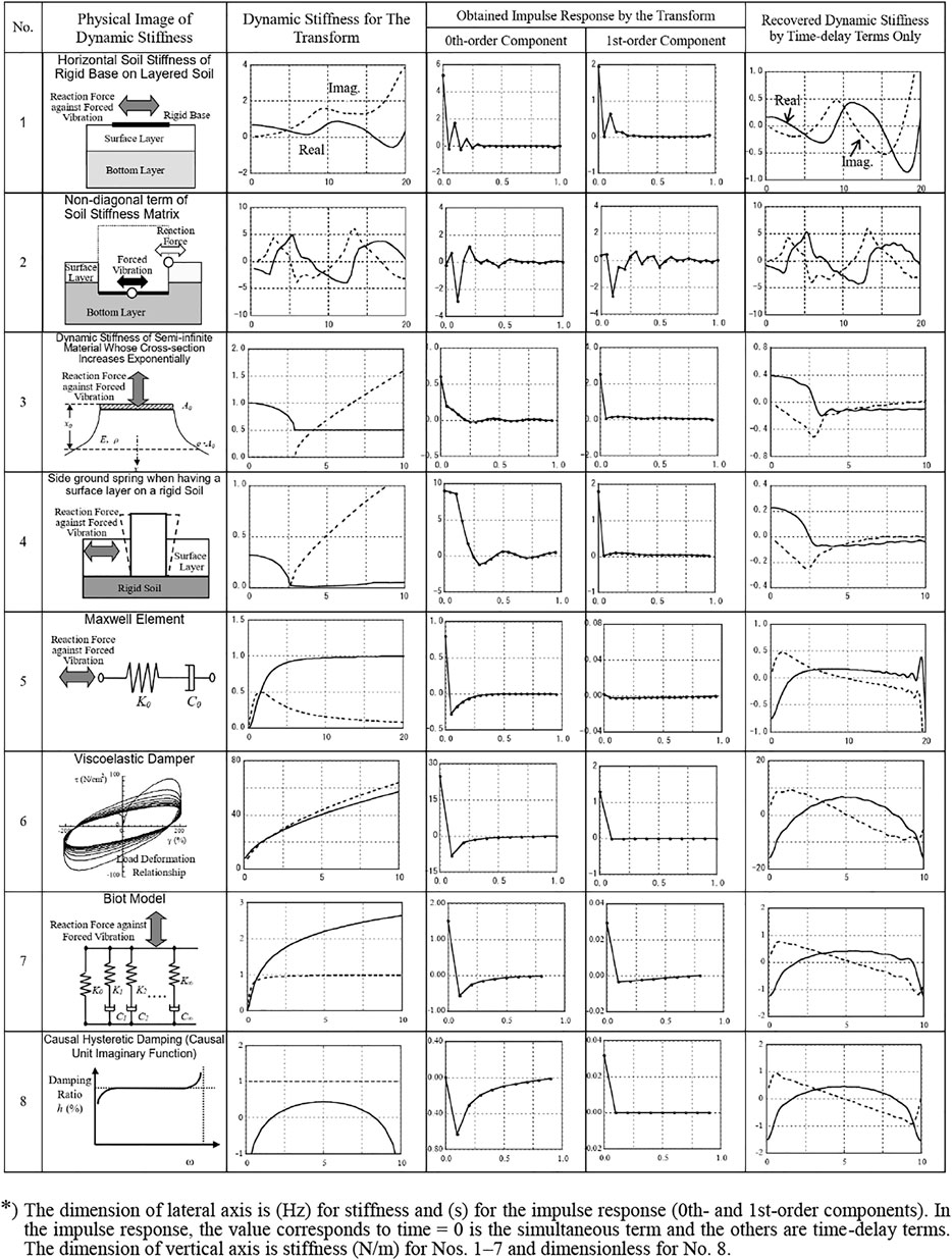
FIGURE 1. Typical transform examples for time-domain transform. * The dimension of lateral axis is (Hz) for stiffness and (s) for the impulse response (0th- and 1st-order components). In the impulse response, the value corresponds to time = 0 is the simultaneous term and the others are time-delay terms. The dimension of vertical axis is stiffness (N/m) for Nos. 1–7 and dimensionless for No. 8.

For all figures, the dimension of the vertical axis is stiffness (N/m) for Nos. 1–7 and dimensionless for No. 8.

These eight problems can be classified into the following three types according to the impulse response characteristics. Below, we analyze and organize each problem.

(1) Horizontal ground impedance (dynamic stiffness) of layered soil (Nos. 1 and 2).

(2) Ground impedance with cut-off frequency (Nos. 3 and 4).

(3) Maxwell element, viscoelastic body, and similar impedance (Nos. 5–8)

Ground Impedance of Layered Soil (Nos. 1 and 2)

No. 1 is the horizontal ground impedance of the rigid base on the two-layered soil. Figure 2 shows its soil properties. No. 2 is the off-diagonal component of the ground impedance matrix of the building embedded in the two-layered soil. That component corresponds to the reaction force at the ground point position when forced vibration is performed on the rigid base at the bottom of the structure. Both impedances are greatly wavy. The rightmost column of the figure shows the impedance recovered using only the time-delayed terms, which is the main cause of frequency dependency; thus, periodic vibration appears clearly.

FIGURE 2

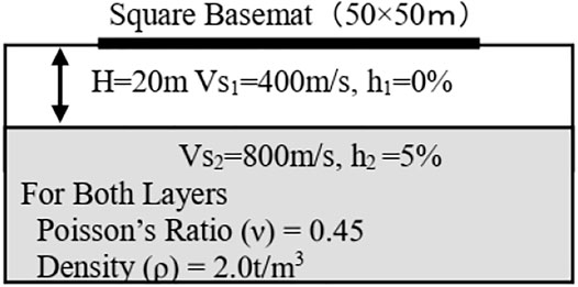
FIGURE 2. Soil properties for No. 1.

As for No. 1, in the impulse response obtained using the time-domain transform, pulses are generated at 0.1 s for the 0th- and 1st-order components. This time-delay can be considered as follows. A wave generated by the forced vibration of the rigid base at the soil’s surface propagates underground. If it is uniform soil, it will dissipate as it is. However, in layered soil, the wave is reflected at the boundary of the bottom layer and comes back. A reaction force is generated to shake the rigid base again. This appears as a time-delay term of the impulse response, and the time-delay corresponds to the round-trip time of the wave. In this ground model, the shear wave velocity Vs of the surface layer is 400 m/s. The surface layer thickness is 20 m, so the wave trips 40 m, and the time delay is 0.1 s.

In No. 2, it is considered that the wave generated by the vibration at the midpoint position propagates in the ground, reaches the ground surface position, and corresponds to the reaction force that tries to shake the point. The time delay of 0.1 s in this model is considered the time required for wave propagation from the midpoint to the ground surface. The Vs of the surface layer is 200 m/s, and the surface layer thickness is 20 m for this problem. Because the reaction force does not occur simultaneously as the vibration, the simultaneous terms do not appear (although a minute value appears, it is considered a numerical cause). Consequently, the impedance becomes a property close to the periodic harmonic wave. Periodic vibration corresponding to the time mentioned above delay is often seen in the off-diagonal components of the impedance matrix.

Another common characteristic of Nos. 1 and 2 is that the effect of the time-delay terms of the 1st-order compnents cannot be ignored. For such problems, the proposed method using two types of impulse responses, the 0th- and 1st-order components, is considered particularly useful. For other impedances (Nos. 3–8), the time-delay terms of 1st-order component are small.

Ground Impedance With Cut-Off Frequency (Nos. 3 and 4)

No. 3 is the dynamic stiffness at the top of a semi-infinite material whose cross-section increases exponentially (Wolf and Motosaka, 1985) and has a cut-off frequency. It is a typical example of the problem that the radiation damping is almost 0 below a certain frequency. In this problem, the theoretical value of the impulse response and impedance are obtained. Impedance S(ω) and impulse response G(t) are shown using Eqs 16, 17, respectively.

$S\left(\omega \right)=\frac{E·A_0}{2x_0}\left(1+\sqrt{1-4a_0^2}\right)(16)$

$\begin{array}{l}G\left(t\right)=\frac{E·A_0}{x_0}\left(\frac{1}{2}\delta \left(t\right)+\frac{x_0}{C_0}·\frac{d\left(\delta \left(t\right)\right)}{dt}+\frac{1}{2t}{J}_1\left(\frac{C_0}{x_0}·t\right)\right)\\ a_0=\frac{\omega ·x_0}{C_0},C_0=\sqrt{\frac{E}{\rho }}\end{array}(17)$

Where,

Here, E denotes the Young’s modulus; ρ denotes the mass density; and J₁ denotes the first-order Bessel function. The first and second terms of Eq. 17 correspond to the simultaneous terms of the proposed methods ₀h₀ and ₁h₀, respectively. The third term corresponds to the time-delay terms of the 0th-order component.

The theoretical value of the impulse response in Eq. 17 is given as a continuous quantity concerning time t, whereas the impulse response obtained the proposed methods is discrete values for each Δt. Therefore, the theoretical value was converted using Eq. 18, and it was confirmed that the impulse response obtained using the proposed method corresponds well to this.

$G\prime \left(t_j\right)={\displaystyle {\int }_{t_j-\frac{\Delta t}{2}}^{t_j+\frac{\Delta t}{2}}G\left(t\right)dt}\left(t_j=\Delta t·j\right)(18)$

No. 4 is the dynamic stiffness of the side of the massless rigid cylinder embedded in the viscoelastic surface layer on the rigid soil and is known as a problem having a cut-off frequency similar to No. 3. Tajimi (1969) performed a rocking vibration analysis of rigid foundations and calculated theoretical solutions. Harada et al. (1983) improved this and expressed it as a spring per unit layer thickness in the underground sidewall and showed that this distribution became almost constant in the depth direction.

Eq. 19 shows the impedance of the Harada’s spring. Here, H denotes the surface layer thickness; Vs denotes the surface shear wave velocity; r₀ denotes the equivalent radius of the foundation; μ denotes the shear modulus of the ground; h denotes the damping ratio of the layer; ν denotes the Poisson’s ratio; and Kn (ω) denotes the nth order of the modified Bessel function.

$K_H\left(\omega \right)=\frac{8r_0^2\mu }{H^2}·{\displaystyle \sum _n^N\frac{{\xi }_n^2·{\Omega }_n}{n^3}·{\left(-1\right)}^{\frac{n-1}{2}}\left(n=\mathrm{1,3,5}\dots N\right)}(19)$

Where,

$\begin{array}{l}{\mathrm{\Omega }}_n=\frac{4K_1\left({\gamma }_R\right)K_1\left({\beta }_R\right)+{\beta }_R{K}_1\left({\gamma }_R\right)K_0\left({\beta }_R\right)+{\gamma }_n{K}_0\left({\gamma }_R\right)K_1\left({\beta }_R\right)}{\left[{\gamma }_R{K}_0\left({\gamma }_R\right)+K_1\left({\gamma }_R\right)\right].\left[{\beta }_R{K}_0\left({\beta }_R\right)+K_1\left({\beta }_R\right)\right]-K_1\left({\gamma }_R\right)K_1\left({\beta }_R\right)}\\ {\beta }_R={\beta }_n{r}_0,{\gamma }_R={\gamma }_n{r}_0\\ {\beta }_n=\frac{\pi }{2H}·\frac{1}{\sqrt{1+2i·h}}·{\xi }_n,{\gamma }_n=\frac{\pi }{2H}·\sqrt{\frac{1-2\nu }{2\left(1+\nu \right)}}·{\xi }_n\\ {\xi }_n=\sqrt{\left(1+2i·h\right)n^2-{\left(\omega /{\omega }_g\right)}^2},{\omega }_g=\frac{\pi Vs}{2H}\end{array}\}(20)$

The impulse responses of Nos. 3 and 4 show almost the same properties. The 0th-component of the impulse response has simultaneous term and time-delay terms. The latter converges to 0 while oscillating as the time delay increases. The 1st-component has almost simultaneous terms only. Even in the impedance recovered using only the time-delay terms, Nos. 3 and 4 have almost the same shape.

Maxwell Element, Viscoelastic Body, and Similar Impedance (Nos 5–8)

The Maxwell element of No. 5 is a spring (K₀) and a dashpot (C₀) connected in series and its characteristics are expressed using the relaxation, shown in Figure 3 time τ_r = C₀/K₀. Further, the impedance is expressed using Eq. 21. When ω = 0, the real part and the imaginary part become 0, and when ω → ∞, the real part becomes K₀, and the imaginary part gradually approaches K₀/(τ_rω). Eq. 22 provides the theoretical impulse response, and the simultaneous and time-delay terms are only in the 0th-component. Similar to No. 3, the theoretical impulse response value was converted to a discrete value using Eq. 18. It was confirmed that the impulse response obtained using the proposed method corresponds well to this.

$S\left(\omega \right)=K_0\left(1-\frac{\frac{1}{{\tau }_r}}{i\omega +\frac{1}{{\tau }_r}}\right)(21)$

$G\left(t\right)=K_0\left(\delta \left(t\right)-\frac{e^{-\frac{t}{{\tau }_r}}}{{\tau }_r}\right)(22)$

FIGURE 3

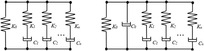
FIGURE 3. Examples of the generalized Maxwell elements.

No. 6 is a constitution rule identified by Kasai et al. (2004) from the experimental results of acrylic materials. The storage stiffness G'(ω) and loss coefficient η(ω) are expressed using Eqs 23, 24, respectively. The parameters of this material are obtained as a = 5.60 × 10^–5, b = 2.10, μ = 3.92 × 10² N/m², and α = 0.558.

$G^{\prime }\left(\omega \right)=\mu \frac{1+ab{\omega }^{2\alpha }+\left(a+b\right){\omega }^{\alpha }\cos \left(\alpha \pi /2\right)}{1+a^2{\omega }^{2\alpha }2+a{\omega }^{\alpha }\cos \left(\alpha \pi /2\right)}(23)$

$\eta \left(\omega \right)=\frac{\left(-a+b\right){\omega }^{\alpha }\sin \left(\alpha \pi /2\right)}{1+ab{\omega }^{2\alpha }+\left(a+b\right){\omega }^{\alpha }\cos \left(\alpha \pi /2\right)}(24)$

No. 7 is the Biot model (Biot, 1958), the limit of the generalized Maxwell element. The 0th-order component of the impulse response is similar to Nos. 5 and 6.

No. 8 is a time-domain approximation of the unit imaginary function obtained using the transform of the imaginary unit i from the frequency to time domain. This is the main component of the damping models with small frequency dependency as the causal history damping model (Nakamura, 2007) and the extended Rayleigh damping model (Nakamura, 2016). The applicability of these models to practical problems was examined (Nakamura, 2019; Mogi et al., 2021; Ota et al., 2021).

The impulse responses of Nos. 5–8 obtained via transform have the following characteristics.

1) For the 0th-order component, the time-delay term becomes a significant value, which occurs on the negative side of the figure and converges to 0 as the time delay increases. The simultaneous term is a positive and significant value in Nos. 5–7, but 0 in No. 8.

2) In the 1st-order component, the time-delay term is almost 0.

Consequently, the impedances of Nos. 5–8 recovered only using the time-delay term have similar shapes. It is considered that these frequency dependences are of the same type. The viscoelastic damper of No. 6 is often approximated using the generalized Maxwell element of No. 8, consistent with this result.

The time-domain transform could perform with generally good accuracy in any problem in this section. Table 1 summarizes the properties of the impulse responses transformed for each problem. X in the figure indicates that each component plays an important role in the impulse response.

TABLE 1

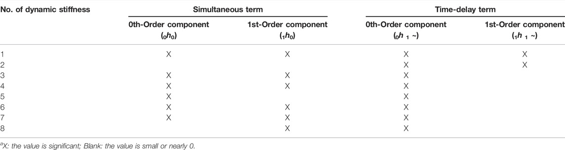
TABLE 1. Components of each case in the time domain.

Regarding the time-delay term related to frequency dependency, the 0th-order component was indispensable in all the problems examined while the 1st-order component was not necessary in many cases. However, it was shown that the 1st-order component is also important in the impedance of the foundation of layered soil (Nos. 1 and 2). It is considered that this is because their dynamic stiffness tends to increase the amplitude of vibration as the frequency increases, and the 1st-order component is required to express this property.

Furthermore, most problems show either the 0th- or 1st-order component for simultaneous terms. This indicates that many dynamic stiffnesses are related to the current displacement or velocity. The exception is No. 2. This corresponds to the fact that the reaction force does not occur simultaneously. This soil stiffness corresponds to the reaction force from where the forced vibration is applied at different places. Therefore, it needs some time that the effect propagates to a different place.

Conclusion

Herein, the following studies were conducted. First, the outline of the transform Methods A to C proposed so far was shown in more general expressions and their characteristics were analyzed and organized. When the noncausality of the dynamic stiffness in the frequency domain is weak, Method B is recommended. When the hysteretic damping of the dynamic stiffness is large, the stiffness has a strong and considerable noncausality; for this case, Method C is recommended.

Next, the above time-domain transform methods were applied to eight typical problems with frequency dependence and their properties were examined. All dynamic stiffnesses could be transformed well, and the effectiveness of the transform method was confirmed. For all problems, it was found that in the time-delay terms related to frequency dependence, the 0th-order component was essential. Moreover, they were roughly classified into three types, and the characteristics of them are as follows:

1) The ground impedance of layered soil (Nos. 1 and 2)

The time delay corresponds to the wave propagation time, so the physical meaning of the time delay is clear. Because the vibration amplitude tends to increase as the frequency increases, the time-delay terms of the 1st-order component are important to represent it.

2) Ground impedance with cut-off frequency (Nos. 3 and 4)

The 0th-order component has simultaneous and time-delayed terms. The latter converges to 0 while oscillating as the time delay increases. The 1st-order component has almost simultaneous terms only. Even in the impedance recovered using only the time-delay term, Nos. 3 and 4 have almost the same shape.

3) Maxwell element, viscoelastic body, and similar impedance (Nos. 5–8).

For the 0th-order component, the time-delay terms become significant values, which occur on the negative side of the figure and converge to 0 as the time delay increases. For the 1st-order component, the time-delay term is small.

It is considered these findings useful for understanding the properties and physical meanings of dynamic stiffnesses with frequency dependence in the time domain. Through these studies, if the frequency dependency of the dynamic stiffness is stable, it is considered that there is no major problem with this transform method. However, if the frequency dependency change largely due to strain or temperature dependency, it is necessary to interpolate and use the transformed results according to the strain and temperature changes. However, it requires a considerable calculation effort; therefore, it is necessary to improve practical methods for such problems.

Data Availability Statement

The raw data supporting the conclusion of this article will be made available by the authors, without undue reservation.

Author Contributions

NN contributed to conception, design of the study, and wrote the first draft of the manuscript. KN, YM, and AO checked and advised to improved the manuscript. All authors contributed to manuscript revision, read, and approved the submitted version.

Conflict of Interest

Authors YM and AO are employed by Taisei Corporation.

The remaining authors declare that the research was conducted in the absence of any commercial or financial relationships that could be construed as a potential conflict of interest

Publisher’s Note

All claims expressed in this article are solely those of the authors and do not necessarily represent those of their affiliated organizations, or those of the publisher, the editors and the reviewers. Any product that may be evaluated in this article, or claim that may be made by its manufacturer, is not guaranteed or endorsed by the publisher.

References

Biot, M. A., (1958), Linear Thermodynamics and the Mechanics of the Solid. In Proc. 3rd US National Congress of Applied Mechanics, ASCE, 1–18.

Google Scholar

de Barros, F. C. P., and Luco, J. E. (1990). Discrete Models for Vertical Vibrations of Surface and Embedded Foundations. Earthquake Engng. Struct. Dyn. 19, 289–303. doi:10.1002/eqe.4290190211

CrossRef Full Text | Google Scholar

Harada, T., Kubo, K., Katayama, T., and Hirose, T. (1983). Dynamic Stiffness of Embedded Cylindrical Rigid Foundation. Proc. Jpn. Soc. Civil Eng. 1983, 79–88. doi:10.2208/jscej1969.1983.339_79

CrossRef Full Text | Google Scholar

Hayashi, Y., and Katukura, H. (1990). Effective Time-Domain Soil-Structure Interaction Analysis Based on FFT Algorithm with Causality Condition. Earthquake Engng. Struct. Dyn. 19, 693–708. doi:10.1002/eqe.4290190506

CrossRef Full Text | Google Scholar

Hsu, H. P. (1967). Fourier Analysis. New York, U.S.A: Simon & Schuster.

Google Scholar

Kasai, K., Ooki, Y., Tokoro, K., Amemiya, K., and Kimura, K. (2004). JSSI Manual for Building Passive Control Technology, Time-History Analysis Model for Viscoelastic Dampers, 13th World Conference on Earthquake Engineering. Vancouver, Canada: IAEE. part 9.

Google Scholar

Kirekawa, A., Ito, Y., and Asano, K., (1992). A Study of Structural Control Using Viscoelastic Material, 10^th World Conference of Earthquake Engineering, 2047-2054.

Google Scholar

Makris, N., and Constantinou, M. C. (1991). Fractional‐Derivative Maxwell Model for Viscous Dampers. J. Struct. Eng. 117, 2708–2724. doi:10.1061/(asce)0733-9445(1991)117:9(2708)

CrossRef Full Text | Google Scholar

Meek, J. W. (1990). Recursive Evaluation of Dynamic Phenomenon in Civil Engineering. Bautechnik 67, 205–210.

Google Scholar

Mogi, Y., Nakamura, N., and Ota, A. (2021). Application of Extended Rayleigh Damping Model to 3D Frame Analysis. Nihon Kenchiku Gakkai Kozokei Ronbunshu 86, 738–748. doi:10.3130/aijs.86.738

CrossRef Full Text | Google Scholar

Motosaka, M., and Nagano, M. (1992). Recursive Evaluation of Convolution Integral in Nonlinear Soil-Structure Interaction Analysis and its Applications. J. Struct. Construction Eng. 436, 71–80. doi:10.3130/aijsx.436.0_71

CrossRef Full Text | Google Scholar

Nakamura, N. (2019). Application of Causal Hysteretic Damping Model to Nonlinear Seismic Response Analysis of Super High-Rise Building. J. Struct. Construction Eng. (Transactions AIJ) 759, 627–637. doi:10.3130/aijs.84.597

CrossRef Full Text | Google Scholar

Nakamura, N. (2016), Extended Rayleigh Damping Model, Front. Built Environ. 2, doi:10.3389/fbuil.2016.00014

CrossRef Full Text | Google Scholar

Nakamura, N. (2006a). A Practical Method to Transform Frequency Dependent Impedance to Time Domain. Earthquake Engng Struct. Dyn. 35, 217–231. doi:10.1002/eqe.520

CrossRef Full Text | Google Scholar

Nakamura, N. (2012). Basic Study on the Transform Method of Frequency-dependent Functions into Time Domain: Relation to Duhamel's Integral and Time-Domain-Transfer Function. J. Eng. Mech. 138, 276–285. doi:10.1061/(asce)em.1943-7889.0000330

CrossRef Full Text | Google Scholar

Nakamura, N. (2006b). Improved Methods to Transform Frequency-dependent Complex Stiffness to Time Domain. Earthquake Engng Struct. Dyn. 35, 1037–1050. doi:10.1002/eqe.570

CrossRef Full Text | Google Scholar

Nakamura, N. (2008b). Nonlinear Response Analysis Considering Dynamic Stiffness with Both Frequency and Strain Dependencies. J. Eng. Mech. 134, 530–541. doi:10.1061/(asce)0733-9399(2008)134:7(530)

CrossRef Full Text | Google Scholar

Nakamura, N. (2007). Practical Causal Hysteretic Damping. Earthquake Engng Struct. Dyn. 36, 597–617. doi:10.1002/eqe.644

CrossRef Full Text | Google Scholar

Nakamura, N. (2008a). Seismic Response Analysis of Deeply Embedded Nuclear Reactor Buildings Considering Frequency-dependent Soil Impedance in Time Domain. Nucl. Eng. Des. 238, 1845–1854. doi:10.1016/j.nucengdes.2007.12.006

CrossRef Full Text | Google Scholar

Ota, A., Nakamura, N., and Mogi, Y. (2021). Examination of Applicability of Causality-Based Damping Model to Dynamic Explicit Method. Nihon Kenchiku Gakkai Kozokei Ronbunshu 86, 1168–1179. doi:10.3130/aijs.86.1168

CrossRef Full Text | Google Scholar

Saitoh, M. (2007). Simple Model of Frequency-dependent Impedance Functions in Soil-Structure Interaction Using Frequency-independent Elements. J. Eng. Mech. 133, 1101–1114. doi:10.1061/(asce)0733-9399(2007)133:10(1101)

CrossRef Full Text | Google Scholar

Tajimi, H., (1969), Dynamic Analysis of Structure Embedded in an Elastic Stratum, Proc. 4th World Conference on Earthquake Engineering, A-6, 53–69.

Google Scholar

Wolf, J. P., and Motosaka, M. (1989). Recursive Evaluation of Interaction Forces of Unbounded Soil in the Time Domain. Earthquake Engng. Struct. Dyn. 18, 345–363. doi:10.1002/eqe.4290180304

CrossRef Full Text | Google Scholar

Wolf, J. P., and Obernhuber, P. (1985). Non-linear Soil-Structure-Interaction Analysis Using Dynamic Stiffness or Flexibility of Soil in the Time Domain. Earthquake Engng. Struct. Dyn. 13, 195–212. doi:10.1002/eqe.4290130205

CrossRef Full Text | Google Scholar

Wolf, J. P. (1997). Spring-Dashpot-Mass Models for Foundation Vibrations. Earthquake Engng. Struct. Dyn. 26, 931–949. doi:10.1002/(sici)1096-9845(199709)26:9<931::aid-eqe686>3.0.co;2-m

CrossRef Full Text | Google Scholar

Wu, W.-H., and Lee, W.-H. (2002). Systematic Lumped-Parameter Models for Foundations Based on Polynomial-Fraction Approximation. Earthquake Engng. Struct. Dyn. 31, 1383–1412. doi:10.1002/eqe.168

CrossRef Full Text | Google Scholar

Xue, S. t., Tobita, J., Hanzawa, T., and Izumi, M. (1992). Wave Attenuation in Viscoelastic Continuum with Fading Memory. J. Eng. Mech. 118, 1597–1611. doi:10.1061/(asce)0733-9399(1992)118:8(1597)

CrossRef Full Text | Google Scholar