 Javier Arroyo
 Fred Spiessens2,3
 Lieve Helsen
94% of researchers rate our articles as excellent or good
Learn more about the work of our research integrity team to safeguard the quality of each article we publish.
Find out more
ORIGINAL RESEARCH article
Front. Built Environ., 01 April 2022
Sec. Indoor Environment
Volume 8 - 2022 | https://doi.org/10.3389/fbuil.2022.849754
This article is part of the Research TopicGlobal Excellence in Indoor Environment: 'Europe'View all 4 articles
Optimal controllers can enhance buildings’ energy efficiency by taking forecast and uncertainties into account (e.g., weather and occupancy). This practice results in energy savings by making better use of energy systems within the buildings. Even though the benefits of advanced optimal controllers have been demonstrated in several research studies and some demonstration cases, the adoption of these techniques in the built environment remains somewhat limited. One of the main reasons is that these novel control algorithms continue to be evaluated individually. This hampers the identification of best practices to deploy optimal control widely in the building sector. This paper implements and compares variations of model predictive control (MPC), reinforcement learning (RL), and reinforced model predictive control (RL-MPC) in the same optimal control problem for building energy management. Particularly, variations of the controllers’ hyperparameters like the control step, the prediction horizon, the state-action spaces, the learning algorithm, or the network architecture of the value function are investigated. The building optimization testing (BOPTEST) framework is used as the simulation benchmark to carry out the study as it offers standardized testing scenarios. The results reveal that, contrary to what is stated in previous literature, model-free RL approaches poorly perform when tested in building environments with realistic system dynamics. Even when a model is available and simulation-based RL can be implemented, MPC outperforms RL for an equivalent formulation of the optimal control problem. The performance gap between both controllers reduces when using the RL-MPC algorithm that merges elements from both families of methods.
Industry, transportation, and buildings are responsible for the largest share of greenhouse gases (GHG) emitted into the atmosphere. According to the International Energy Agency (IEA), the United Nations Environment Programme, and the Global Alliance for Buildings and Construction, the CO2 emissions associated with the building sector account for 38% of the global energy-related CO2 emissions (lobalnvironmen, 2020), corresponding to 13.6 Gt CO2-eq/year. According to a report delivered by the same organization (lobalnvironmen, 2019), above half of the energy used in buildings is used by the heating, ventilation, and air conditioning (HVAC) systems for space heating, space cooling, and water heating. Figure 1 highlights that buildings are the largest emitters. Moreover, unlike industry and transportation, the building sector offers an untapped potential to improve the control strategies used for their operation.
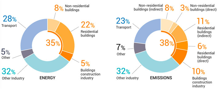
FIGURE 1. Global share of buildings and construction final energy and emissions, 2019. Figure obtained from (lobalnvironmen, 2020).
The massive energy savings potential in buildings stems from their longevity, risk-averse industry, and large thermal inertia. The long lifespan of buildings results in a building stock that requires renovation. Their materials degrade, and their HVAC systems become deprecated. Even for new constructions, building owners and operators usually stick to classical rule-based controls and have not yet widely adopted advanced methods integrating prediction and optimization that have the potential to enhance operational efficiency (Drgoňa et al., 2020).
Furthermore, the large thermal inertia of buildings enables flexible operation, an appealing feature when connected to an electric grid with a rise of intermittent renewable energy sources (RES) such as wind and solar power. Buildings can provide demand response (DR) services through power-to-heat devices like heat pumps or electric heaters. The building sector is particularly suitable for providing DR because it accounts for approximately 55% of the global electricity use (lobalnvironmen, 2020). Besides, their constructions and indoor spaces constitute an infrastructure already in place with an invaluable potential to steer flexibility. Intelligent building operation can harvest this flexibility by implementing modeling, commissioning, and predictive control.
Ensuring building indoor comfort and safe operation while enhancing energy efficiency and providing flexibility is an exceptionally complex control problem. Buildings comprise several variables and a wide variety of time constants. Set-points and actuator values need to be decided for every control step and building HVAC component based on a few measurements. Additionally, the effect of a decision may be well delayed in time.
Optimal control is a mature science that solves a sequential decision-making problem to determine the control actions that optimize a performance objective. The applicability of optimal control is clear, and it has been implemented in multiple fields like medicine, engineering, psychology, or economics. During the last decade, there has been a clear interest growth in using optimal control for HVAC systems because it provides the theory to address the challenges mentioned above. Figure 2 underlines this increased interest by showing the number of yearly peer-reviewed scientific publications related to optimal control in buildings.
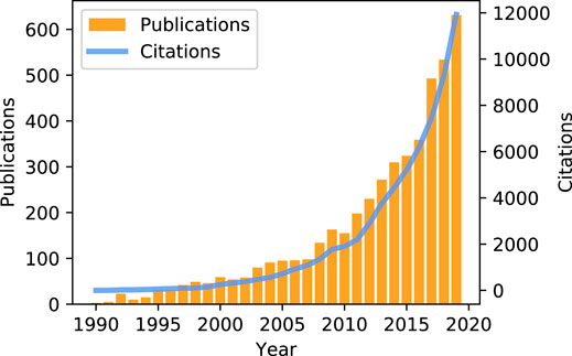
FIGURE 2. Evolution of the number of scientific publications about optimal control in buildings during the last decades. Data obtained from the Clarivate Web of Science.
Model predictive control (MPC) and reinforcement learning (RL) are two approaches for optimal control that pursue the same goal but follow different strategies. The MPC approach is mainly studied within the control theory community, and it is well known for its robustness and sample efficiency but falls short in terms of adaptability. It usually requires a significant engineering effort to implement and configure a controller model suitable for optimization. On the other hand, RL is mainly studied within the machine learning community. Contrarily to MPC, this advanced control approach is well known for its adaptability and versatility, but it has difficulties dealing with constraints and lacks intelligibility. Both control families have advantages and disadvantages, and the complementarity between them is clear. However, it is unclear if there is one method more suitable than the other for the application of building energy management (BEM). Moreover, the hyperparameters of the controllers are typically obtained based on experience and heuristics. Particularly for RL, the choice of hyperparameters is arbitrary, primarily because of the black-box nature of this optimal control technique. The control parameters to be tuned in the RL approach have no physical interpretation, which makes it difficult to draw general guidelines for the design of a learning agent.
A unified benchmarking framework is thus required to facilitate a fair evaluation of the algorithms and shed light on best practices for optimal control in buildings. The Building Optimization Testing (BOPTEST) framework (Blum et al., 2021) has been recently developed specifically to address that need: the evaluation and benchmarking of different control techniques for BEM. The framework provides a simulation environment with a menu of emulator building models that come along with standardized test cases and baseline controllers that serve as a performance reference. The framework also provides functionality to compute Key Performance Indicators (KPIs), read and overwrite control points, and handle boundary condition data like weather or pricing variables. The BOPTEST application programming interface is general to any controller, but an OpenAI-Gym environment (Arroyo et al., 2021) has been developed around this interface to facilitate the assessment of RL algorithms for building control.
This paper evaluates and benchmarks variations of MPC and RL algorithms with different hyperparameter settings for the BESTEST Hydronic Heat Pump case of the BOPTEST framework. Variations of the control step, prediction horizon, state-action spaces, learning algorithm, and the RL agent network architecture are explored and evaluated in all testing scenarios offered by the envisaged BOPTEST case. The RL-MPC algorithm proposed in our prior work (Arroyo et al., 2022) that merges elements from both MPC and RL is also tested in all available testing scenarios. The objective is to benchmark these methods, and to investigate whether there is any realization of an RL algorithm that can compete against MPC for direct building thermal control when tested in an emulator model with realistic building dynamics.
This paper is structured as follows. Section 2 highlights previous research related to this work; Section 3 explains the methodology used to implement the control algorithms and compare their performance results; Section 4 presents the simulation results; Finally, Section 6 draws the main conclusions of this paper.
In our prior work (Arroyo et al., 2022) we applied MPC, RL, and RL-MPC to the same BOPTEST building case. It was found that RL can difficultly cope with constraints and that RL-MPC could aid in this task. The RL agent from that work was designed to replicate a control formulation equivalent to a typical MPC design, regardless of the state-action space dimension. However, large state-action space dimensions can be challenging to learn because of the curse of dimensionality (Sutton and Barto, 2018). Therefore, other hyperparameter settings could be more effective when training an RL agent. In this paper we investigate whether any of those combinations could outperform MPC. Moreover, previous studies have stressed the need to compare different RL algorithms and test different control parameters in a standardized building benchmark (Touzani et al., 2021).
Other researchers have compared different optimal control techniques and their hyperparameter settings for BEM. For instance, Mbuwir et al. (Mbuwir et al., 2019a) explored two model free offline RL techniques, namely Fitted Q-Iteration (FQI) and policy iteration in a residential micro-grid that integrates a heat pump and a battery. Their work shows that policy iteration is more suitable when developing control policies that control flexibility providers as it results in a lower net operational cost per day. A comparison against MPC was also performed in this case study indicating that the RL algorithms are a viable alternative to MPC, although their focus was on the operation of a micro-grid rather than optimal building climate control. For this reason, the thermal behavior of the indoor building space was oversimplified and the same model was used to train and test the agent’s policy. No partial observability was considered in the study, and discomfort was not explicitly computed as a KPI. Mbuwir et al. (Mbuwir et al., 2019b) further benchmarked different regression methods for function approximation in RL. Six well-known regression algorithms were compared for use in Fitted-Q iteration (FQI), a batch RL technique, to optimize the operation of a dwelling with a heat pump, PV generation and a battery. It was found that extra-trees combined with FQI can provide a good compromise between accuracy and computational time. Again, the emulator model was oversimplified and partial observability was thus not addressed.
On a similar note, Ruelens et al. (Ruelens et al., 2017) compared batch RL to temporal difference techniques and suggested that batch RL techniques are more suitable for their application to DR. Their simulation study showed that RL combined with a Long-Short Term Memory (LSTM) performed better than other classical function approximations like neural networks. However, their analysis was again exclusively based on operational cost and did not consider thermal discomfort. A very similar study was carried out by Patyn et al. (Patyn et al., 2018) who explored different topologies of neural networks as function approximators for an RL agent. In their case, the use of Convolutional Neural Networks (CNN), led to significantly higher operational cost than the use of Multi-Layer Perceptron (MLP) or LSTM, which performed similarly.
In general, the research studies that address RL for BEM either use an oversimplified plant model for testing or entail a backup controller to deal with constraint satisfaction of thermostatically controlled loads, e.g., (De Somer et al., 2017; Ruelens et al., 2017; Patyn et al., 2018; Mbuwir et al., 2019a; Mbuwir et al., 2019b; Ruelens et al., 2019). It is important to stress here the importance of direct control, i.e. the control of an actuator point that directly influences a controller variable without any backup controller that can potentially modify its behavior. With direct control, the controller/agent needs to deal with constraint satisfaction. Contrarily, indirect control only suggests actions that can be overwritten by a backup controller, which is ultimately responsible for satisfying constraints. While indirect control provides a more secure operation, it does not exploit the full potential of a predictive controller because the controller can only work at a supervisory level and not at a local-loop level where the range of operational possibilities is broader. Indirect control can be implemented by translating an optimal control problem that is formulated using direct control. However, this practice does not guarantee that the used setpoint translates to the right actuation signal unless the model accurately maps this translation.
The studies mentioned above usually claim that model-free RL agents can learn policies for building climate control from only a few days of operation. However, their agents are tested using first and second-order emulator models or directly precomputing the heat demand. This practice directly conflicts with the findings of Picard et al. (Picard et al., 2017), who emphasized the relevance of using a detailed and reliable plant model when evaluating the building controllers in order not to overestimate their performance. Real implementations of RL for building HVAC control, like those in (Liu and Henze, 2006; Zhang and Lam, 2018; Chen et al., 2019), never use model-free RL techniques directly and rely on simulation-based off-line learning or model-based RL. To the best of our knowledge, only Peirelinck et al. (Peirelinck et al., 2018) has evaluated a model-free RL agent in a simulation environment using a detailed emulator building model. However, they used indirect control and a low-dimensional action space. Their analysis is thus based on operational cost only and does not take into account thermal discomfort.
None of the above studies has compared variations of MPC and RL techniques in a unified benchmarking framework for BEM. In this study, we investigate direct control for BEM and use the BOPTEST framework for testing, which ensures both reliability of the plant model and reproducibility of the results. The most favorable case scenario for the data-driven methods is considered by assuming that the RL algorithms can access the plant model with realistic dynamics for a large number of interactions during training.
At the time of writing, the BOPTEST platform comprises five building emulators. The BESTEST Hydronic Heat Pump case from BOPTEST as in version v0.1.0 is used in this study to investigate the performance of several optimal control implementations. This test case offers a representative, yet relatively simple, building model that allows focusing on fundamental aspects of the control problem. The following description of the test case is based on the explanation gien by Blum et al. (Blum et al., 2021) and it is partially repeated here for clarity.
The test case model represents a single-zone residential building with a hydronic radiant floor heating system and an air-source heat pump located in Brussels, Belgium. The building is modeled as a single zone with a rectangular floor plan of 12 m by 16 m (192 m2) and a height of 2.7 m, with a south-oriented façade that has multiple windows with a total surface area of 24 m2. The thermal mass of indoor walls is modeled assuming that there are 12 rooms in the building. The modeled indoor walls do not split the indoor space of the single-zone building model but increase its overall thermal mass.
A family of five members inhabit the building and follows a typical residential weekly schedule, where the building is occupied before 7h00 and after 20h00 every weekday and full time during weekends. The comfort range defines the boundaries of the indoor operative zone temperature and is 21–24°C during occupied hours and 15–30°C otherwise.
The heating system consists of an air-to-water modulating heat pump of 15 kW nominal thermal capacity, which is coupled to a floor heating system. The embedded baseline controller for heat pump modulation uses a PI logic to track the operative zone temperature. This controller, while reactive, has been carefully tuned to provide adequate indoor comfort without excessive energy use. The floor heating circulation pump and evaporator fan operate only when the heat pump is on. No cooling is considered in this test case, which is justifiable in a Belgian climate.
Figure 3 shows a schematic drawing of the BESTEST Hydronic Heat Pump case. Note that only the control points and measurements used in this dissertation are shown in Figure 3, these being a subset of the points exposed in the BOPTEST framework. In Figure 3, ufan, upum, and uhp represent the input signals for controlling the fan, the pump, and the heat pump compressor frequency, respectively. Pfan, Ppum, and Php indicate the measurements of the electric power of the evaporator fan, the circulation pump, and the heat pump compressor.
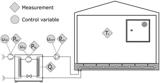
FIGURE 3. Scheme of the BESTEST Hydronic Heat Pump building case.
The building envelope model is implemented using the IDEAS Modelica library (Jorissen et al., 2018) and incorporates, among others: dynamic zone air temperature, air infiltration assuming a constant n50 value, dynamic heat transfer through walls, floor, ceiling, and fenestration, and non-linear conduction, convection, and radiation models. Air humidity condensation and start-up losses are not considered.
This test case comprises two testing periods of 2 weeks each, that are standardized in the BOPTEST framework and that represent typical and peak heating periods. These periods are January 17th-31st and april 19th-May 3rd, respectively. For each of them, three price scenarios are considered, namely: constant, dynamic, and highly-dynamic. The constant price scenario uses a constant price of 0.2535 €/kWh. For the dynamic price scenario the test case uses a dual-rate that alternates between an on-peak price of 0.2666 €/kWh between 7h00 and 22h00, and an off-peak price of 0.2383 €/kWh otherwise. The highly dynamic price scenario uses the Belgian day-ahead energy prices as determined by the BELPEX wholesale electricity market in the year 2019. All pricing scenarios include the same constant contribution for transmission fees and taxes as determined by Eurostat and obtained from (European CommissionDirect, 2020). Particularly, this component is 0.2 €/kWh for the assumed test case location, and only the remainder of the price is the energy cost from the utility company or the wholesale market.
All six available case scenarios are considered in this paper when testing the controllers for a complete overview and evaluation. These scenarios arise from combining the two heating periods (peak and typical) and the three electricity pricing tariffs (constant, dynamic, and highly-dynamic). Each controller instance is tested in each of the 2-weeks scenario periods. The control objective is always the same: maximize comfort while minimizing operational cost. To this end, both the MPCs objective functions and the RL agents’ rewards are configured to weigh discomfort approximately one order of magnitude more than the operational cost at nominal conditions.
MPC is implemented using the FastSim toolbox (Arroyo et al., 2018). Particularly, the nonlinear MPC configuration described in Blum et al., (2021) and in Arroyo et al. (2022) is used, and it is summarized here for completeness. A controller model F is required by the MPC. A grey-box model is used consisting of a thermal resistance-capacitance (RC) architecture constructed from basic physical principles and without using any system metadata like building geometry or material properties. A model of order five is decided from a forward-selection procedure.
The model has a total of 20 lumped parameters that need to be estimated. The parameter estimation process is carried out with the Grey-Box Toolbox (De Coninck et al., 2016). Two weeks of data are generated by the emulator with the baseline controller for training, and 2 weeks are used for validation of the model. The fitting variables are the zone operative temperature Tz, the heat pump condenser thermal power
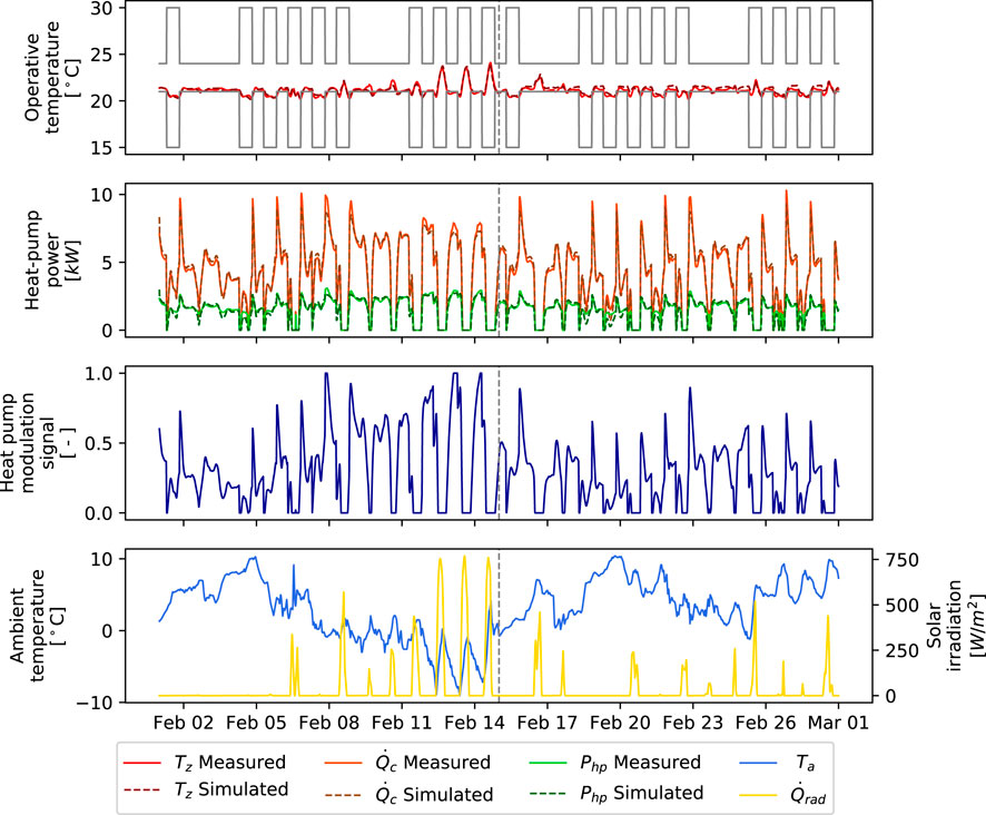
FIGURE 4. Training and validation periods for estimating the controller model F. The training period is at the left of the vertical grey dashed line and the validation period at the right. The inputs are presented in the bottom two plots, and the simulated outputs are presented in the top two plots and compared with the measured data. The grey lines in the first plot represent the comfort constraints.
The non-linear JModelica optimization module developed in (Axelsson et al., 2015) is used here and has been extended to enable mutable external data. This JModelica module utilizes the direct collocation scheme and relies on CasADi (Andersson et al., 2019) for algorithmic differentiation. This approach is well known for its versatility and robustness. The optimization problem that needs to be solved at every control step is formulated in Eq. 1e.
In Eq. 1e and the time dependency has been omitted for clarity because all variables are time-dependent except the vector of model parameters p, and the weighting factor w, the latter being used to account for the different orders of magnitude between energy cost and discomfort
The optimization module is combined with the unscented Kalman filter of the JModelica toolbox for state estimation. The specific state estimation algorithm is the non-augmented version described in (Sun et al., 2009), and the sigma points are chosen according to (Wan and Van Der Merwe, 2000). The controller model F is also used by the state estimator to compute the distribution of predicted model states.
Perfect deterministic forecast provided by BOPTEST is used by the MPC every control step. Variations in the prediction horizon of 3, 6, 12, 24, or 48 h and in the control step of 15, 30, or 60 min are considered. The objective of exploring these variations is twofold: first, to determine the sensitivity of the MPC to these parameters. Second, to extend the benchmarking results of the baseline controller with the results of an optimal predictive controller for the tested RL agents.
The performance results obtained with the different prediction horizons are related to the time constant of the building to enable the generalizability of the conclusions drawn. Usually, the time constant of a building can only be roughly estimated from the step response because the boundary conditions prevent the building from settling fully. A BOPTEST case is also unavoidably exposed to changing boundary conditions. However, the simulation capabilities of the framework can be exploited to obtain a more accurate approximation of the time constant of the building test case. Particularly, the building can be simulated in free-floating from two different initial conditions, e.g., an indoor temperature state higher than another. The difference between the resulting output trajectories represents the system’s step response where the effects of the boundary conditions are mostly filtered out. The resulting trajectory can be used to estimate the time constant τ from its definition in Eq. 1 if a first-order system for the step response is assumed.
The time constant τ is estimated by fitting Eq. 1 to a given evolution of the temperature difference ΔT(t) from an initial temperature difference ΔTi that is artificially generated to emulate the step.
The process of calculating the step response by filtering out the effect of the continuously changing boundary conditions is schematically depicted in Figure 5. In this figure, Tz,high represents the zone operative temperature of the simulation that starts at a higher thermal state, Tz,low represents the zone operative temperature of the simulation that starts at a lower thermal state, and Ta is the ambient temperature.
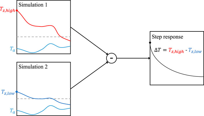
FIGURE 5. Schematic representation of the process used to estimate the building step response in BOPTEST.
This study pays particular attention to the evaluation of RL agents because we are interested in the feasibility of model-free control approaches for their application to BEM. There is an indefinite amount of possible combinations of hyperparameters when configuring an RL agent. Since the learning period of an agent is substantially large, it is not possible to use hyperparameter optimization techniques like Bayesian optimization or random search grid for hyperparameter tuning. A different approach is required to evaluate the effect of using different combinations of hyperparameters. We use the one-at-a-time approach, which consists of varying only one hyperparameter from a reference RL agent configuration each time and studying how the new configuration affects the learning process and the performance results in testing. Varying only one hyperparameter at a time throws light on the effect of varying each aspect of the learning agent.
The original choice of hyperparameter settings is called the reference case (REF), and it is chosen to be the same configuration as the one considered in our prior work (3). This reference case is designed to replicate the MPC problem formulation described above. Each implemented agent varies different aspects from the reference case to investigate which features mostly influence the results and to identify those that expedite learning or lead to more effective policies. Aspects like the state space, the action space, the learning algorithm, or the function approximation are explored, tested, and compared. The BOPTEST-Gym environment developed in (33) allows to easily configure the environments with different observations and actions accessible to the learning agent. The summary of considered cases is shown in Table 1, where a ✓ symbol indicates that the observation is included in the state space and a ✗ symbol indicates that it is excluded. More details about the definition of each specific case are provided in the following subsections. Table 1 anticipates the markers that are used in Section 4 to indicate the results.

TABLE 1. Considered RL agent configurations for comparison. The state space representation is grouped in the set of time variables
Two Gym environments are configured for this study. First, the so-called actual environment
Different sets of observed features are passed to the agent to analyze how it can handle state space representations of different dimensions. The variables considered as possible observations are the time of the week tw, the zone operative temperature Tz, the electricity price signal λ, the lower and upper bounds of the comfort range
A trade-off needs to be found between the state space dimension and the information perceived by the agent. All cases exploring variations of the state space dimension are marked purple in Table 1 and their identifiers start by SS. The cases SS1, SS2, and SS3 vary the observations passed to the agent and are those with the lowest state space dimensions. SS4, SS5, and SS6 use the same observation variables as REF, but vary their prediction horizons to be 3, 6, or 12 h, respectively. Finally, SS7 and SS8 explore variations of the control step for 30 and 60 min, respectively.
The action controlled in the reference case is the heat pump modulation signal for compressor frequency uhp. That is,
The BOPTEST-Gym interface is general to all algorithms that follow the OpenAI-Gym standard, which enables to easily plug the building environment into different learning algorithms. The RL algorithms implemented in this paper are obtained from the Stable Baselines repository (14). The reference case uses Double Deep Q-Network (DDQN) for learning as proposed in (Mnih et al., 2013) and in (van Hasselt et al., 2015). Specifically, a double network is implemented to avoid the overoptimism inherent to Q-learning for large-scale problems (van Hasselt et al., 2015). The network weights are updated following a stochastic gradient descent scheme. A linear schedule is followed for exploration during training such that random actions are taken with a probability that linearly decays from 10 to 1%.
The first variation of this algorithm is AL1 and implements an actor-critic approach, i.e., its learning method approximates both the value and the policy functions. Particularly, the Soft Actor Critic (SAC) described by Haarnoja et al. (Haarnoja et al., 2018) is implemented in this variation. SAC optimizes its stochastic actor in an off-policy approach. Another significant difference of SAC with respect to the DDQN algorithm is that it uses a more sophisticated exploration method based on the maximum entropy principle of RL. This means that the agent seeks maximization of the expected return and the expected entropy. The aim is to encourage the agent to explore the regions of the state-action space that it is less familiar with. SAC features continuous action spaces. Hence, the heat pump modulation signal is not discretized in this case, wich is indicated with an ∞ symbol in Table 1.
The second variation (AL2) from the reference case also uses an actor-critic approach as learning method. Specifically, the algorithm used is the synchronous advantage actor critic (A2C) algorithm, a variant of the asynchronous method (A3C) proposed by Mnih et al. (Mnih et al., 2016). The main difference with the algorithms used in REF and AL1 is that it is an on-policy algorithm, i.e. it explores by sampling actions based on the current version of its policy. It also differs from its predecessor, A3C in that it does not trigger several environments at a time and is more cost-effective when parallelization is not performed, as is the case in this work. The key idea behind A2C is that it follows an updating scheme of the policy function approximation based on fixed-length segments of experience. The stabilizing role of the replay buffer of the DDQN algorithm is substituted by updates that involve multiple segments of experience. Each segment explores a different part of the environment such that each update averages the effect of all segments.
A third (AL3) variation from the reference case explores another very popular deep RL algorithm nowadays, namely the Proximal Policy Optimization (PPO) algorithm, as proposed by Schulman et al. (Schulman et al., 2017). PPO is similar to A2C in that it is also an on-policy algorithm and uses a policy gradient update scheme of its actor. It also extends A2C by implementing a clipped objective to update the parameters of the function approximator representing its policy. The formulation of the clipped objective prevents abrupt changes after policy updates that could hinder convergence.
We refer to (Hill et al., 2018) for the practical implementation of these algorithms. All cases exploring variations of the learning algorithm are marked red.
The reference case implements a Multi-Layer Perceptron (MLP) neural network configured with TensorFlow (Abadi et al., 2015) to represent its state-action value function. The state-action value function is updated every step from a target estimated from the immediate perceived reward and the return estimated with the same action-value function at the expected following state. The network architecture configuration used to represent the state-action value function (or the RL agent policy) is usually chosen to be arbitrarily large. The motivation is to ensure that the function approximator provides enough degrees of freedom to capture the necessary correlations between states, actions, and returns. However, a too large network architecture may preclude convergence as it increases the number of parameters that need to be optimized.
In REF, the network consists of an MLP architecture that contains two hidden layers of 64 neurons each and a rectified linear activation function for the nodes. MLP has outperformed other typical network architectures for a similar application. Particularly, Patyn et al. (Patyn et al., 2018) showed that the use of MLP leads to cost savings in the operation of a building when compared to the use of CNN, and its associated computational cost is about half as large when compared to LSTM. The number of neurons in the input layer is the sum of the state and action spaces, and the output layer estimates the Q-value.
Three variations are explored from the network used in the reference case. The first variation (NN1) reduces the network to use only one hidden layer of 64 neurons. The second envisaged architecture (NN2) further decreases the size of the network by using only one hidden layer of 32 neurons. The third variation (NN3) uses the original network architecture but applies normalization to the intermediate layers. That is, the output of a layer is normalized to improve convergence during training. It is worth mentioning that the AL2 variant also required a reduction of the size of the network architecture from the one used in the reference case (1 instead of 2 hidden layers). The reason is that the original network architecture made this agent diverge at early stage during the training process. All variations exploring the effect of different network architectures are marked green.
Each instance of an RL agent interacts with the BOPTEST building emulator for a number of episodes until the maximum number of steps for training is reached. Each episode lasts for 2 weeks and is initialized with 1 day of simulation. The episodes are not allowed to overlap the testing period of the BOPTEST case to ensure that the model is tested in conditions that have not been encountered during learning. The state and action spaces are always normalized to [ − 1, 1] and the electricity price tariff is chosen to be the one from the highly dynamic price scenario of BOPTEST for training.
Note that it is of interest to find precocial RL agents to be used for actual building climate control implementations. Moreover, in our prior work (3) it was shown no significant improvements for training periods of over 300.000 interaction steps and it was indicated that longer training periods did not necessarily lead to better control performance results during testing. Hence, we set the maximum number of training steps to 300.000.
The actual environment
The RL-MPC algorithm, as described in Arroyo et al. (2022) is also implemented for each of the testing scenario periods. We refer to Arroyo et al. (2022) for details about the algorithm and its implementation, but provide here a brief description for clarity. A high-level representation of the RL-Algorithm is shown in Figure 6, where k is the control step index, m is the vector of measurements,
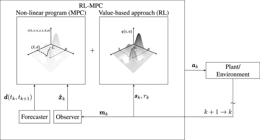
FIGURE 6. Block diagram showing a high-level introduction of RL-MPC. Every control step, RL-MPC decides an action ak by optimizing the sum of the one-step ahead non-linear program of the MPC and the value function from the estimated following state (Arroyo et al., 2022).
RL-MPC is an algorithm that combines elements from MPC and RL. Particularly, the MPC non-linear program that needs to be solved every control step is truncated with the expected one-step ahead value as estimated by as estimated by a value-based RL algorithm. Hence, RL-MPC uses value-based RL to estimate the value of being in a specific state as obtained by the MPC when using a prediction horizon of only one control step. Therefore, the main components of the MPC remain active in RL-MPC, namely the state estimator, forecaster and optimizer, but the value function is used to shorten the non-linear program and to enable learning.
The implementation of the RL-MPC algorithm in this study inherits all attributes and hyperparameters of the REF case, which was defined to be equivalent to the MPC formulation. This means that the same control step, prediction horizon, and state estimator as in the MPC is used. The value function of the RL-MPC algorithm is pretrained with the same DDQN algorithm used to train the RL agents described above. However, in this case we let the agent interact with the simulation environment
Figure 7 shows the control performance results for the baseline controller and for MPC variations in each of the six BOPTEST case scenarios analyzed. In Figure 7, the baseline performance is represented by a green dot, the different prediction horizons are distinguished using different colors, and variations of the control step are indicated by different marker shapes. From the six core KPIs that BOPTEST provides, we show total thermal discomfort and total operational cost per zone, since those are the performance targets of the control problem formulated in this study.
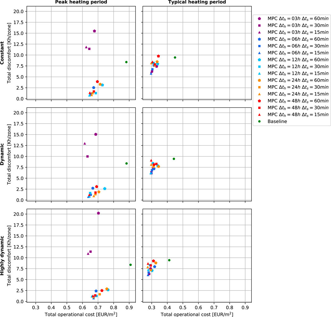
FIGURE 7. MPC performance results for different test case runs in each of the BOPTEST scenarios. The rows show the results for the same pricing scenario, and the columns for the same period scenario. The results are obtained for variations in control step Δts and prediction horizon Δth for the same MPC.
The results show that the baseline controller obtains the same total discomfort independently of the pricing scenario since its control logic ignores the pricing signal. The MPC generally outperforms the baseline controller with discomfort savings up to 90.8% and with cost savings up to 27.2% when using a prediction horizon of 48 h and a control step of 15 min on the peak heat period with dynamic pricing. However, the baseline controller already performs well, and designing the predictive controller to beat the baseline has proven to be a challenging task, especially in terms of operational cost. It is worth noting that the inclusion of the fan and pumping powers in the objective function is key to obtaining operational cost savings. Neglecting these terms makes the MPC working at low partial heat pump load, without considering the low but steady energy use of auxiliary equipment. Another critical aspect to achieve cost savings is to train the controller model not only to fit the zone operative temperature, but also the electrical and thermal powers of the heat pump. This way, the controller model learns an accurate representation of the heat pump COP behavior, which is exploited during operation later on.
More dynamic pricing scenarios only result in small operational cost savings for the typical heating period scenarios. The main reason is that the relative pricing variations are hidden by the high constant pricing component for transportation fees and taxes included in all scenarios, which is relatively large in most of the European countries, including the one where the test case of this example is located. This reduces the monetary incentive to load shifting. Notice that the peak heating scenarios are even less sensitive to pricing variations since they do not offer much freedom to operate without hampering comfort. The exploitation of flexibility is further limited in this test case by higher electricity prices occurring when the ambient temperature is higher, and therefore when the heat pump could benefit from a larger COP.
Shorter control steps usually lead to higher performance, especially for the peak heating period scenarios. The relevance of the prediction horizon length for the peak heat scenario period is clear: a prediction horizon below 6 h is not enough for the MPC to anticipate the thermal load and successfully maintain thermal comfort, although this effect is mitigated by shorter control step periods. Shorter control step periods usually lead to the best performance results for the same scenario and MPC prediction horizon.
The time constant is calculated as explained in Section 3 to generalize these findings. The aim is to find the shortest prediction horizon delivering good performance relative to the time constant of the building, such that other MPC implementations can benefit from this insight. Note that shorter prediction horizons alleviate the computational burden of the online optimization required in implicit MPC. The step response of the zone operative temperature is studied for the envisaged building from 10 different values of the initial temperature difference ΔTi, from 1 up to 10 °C. We choose the peak heating period scenario to carry out the experiments and 20°C as the temperature reference. For each ΔTi, the temperature setpoint is set to be 20 + ΔTi °C during the first 4 days of the testing period, and the emulator is led to free floating for the remaining 10 days by overwriting the heat pump modulation signal: uhp = 0. The temperature trajectory when using a temperature setpoint of 20°C is subtracted from each temperature evolution to eliminate the effect of disturbances.
The temperature response for each temperature difference ΔTi, as determined by the emulator, is shown in Figure 8. In every case, the time constant is estimated by approximating the trajectory by the step response of a first-order system as was shown in Eq. 1. The time constant is taken to be the average of all obtained values, which is 3.03 days with 0.84 h standard deviation. The modeled response is also shown in Figure 8 for each value of ΔTi. Figure 8 shows that when using a reciding horizon the shortest prediction horizon leading to good control performance is 6 h, which is 12 times shorter than the time constant of the building. Longer prediction horizons do not seem to provide added value for this particular building type, as we observe similar results when using the same control step with different prediction horizons.
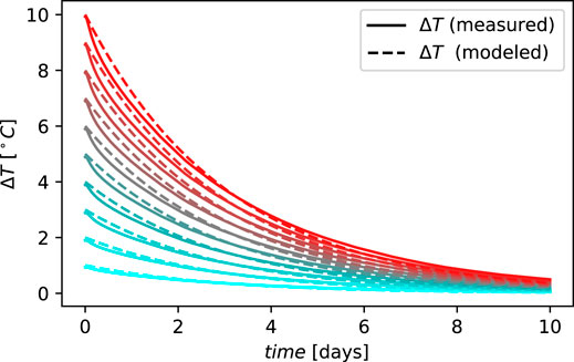
FIGURE 8. Step response evolution of the BESTEST Hydronic Heat Pump case for different values of ΔTi. The “measured” temperature shows the temperature output of the emulator, and the “modeled” temperature shows the output from the system modeled with Eq. 1.
The performance results of the RL agents described in Section 3 are now assessed. First, the learning curves obtained with each agent during training are analyzed. These curves are shown in Figure 9 and they represent the exponential moving average of the episodic return during training. The initial steps of operation determine the initial value of the learning curves during training. Since the RL agents follow a random exploration schedule, it is expected that the initial values vary from one agent to another. A steep curve indicates a fast-learning agent, which means that the associated learning algorithm is sample efficient.
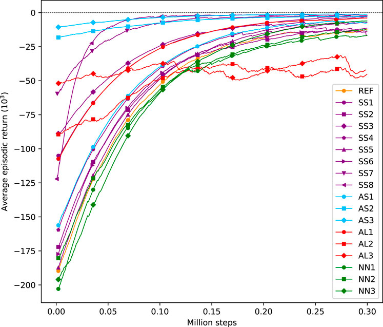
FIGURE 9. Evolution of the average episodic return during learning for each trained agent.
In general, it is observed that the agents tend to increase their expected average episodic return during training, which indicates that they succeed in learning from the interactions with the environment. Only the AL2 and AL3 variants do not show a steady increase in their expected episodic return. These variants correspond to the implementations of the A2C and the PPO algorithms, respectively. Both algorithms differ from the others in that they lack a replay buffer and follow an on-policy method for learning. Note that AL1 implements SAC, which is also another learning algorithm than the one in the reference case (DDQN). However, similarly to DDQN, SAC uses a replay buffer and follows an off-policy method for learning. Contrarily to off-policy algorithms, the exploration of the A2C and the PPO algorithms is based on their policies, which become less random as training progresses. This effect makes them more sensitive to local optima than off-policy algorithms.
SS8 is probably the configuration that leads to the fastest learning, which is logical since it uses the largest control step from all variants, namely Δts = 60 min. A larger control step reduces the size of the state space dimension and, more importantly, it enables the agent to explore longer periods of experience than other agents for the same amount of interaction steps. A similar rationale can be followed for variant SS7 whose steepness is not that outspoken but the agent also benefits from using a longer control step period. Other variations of the observed state space, e.g., reducing the number of observed variables or the forecasting period do not seem to have a major influence on the learning rate. The choice of the neural network architecture used as a function approximator does not significantly influence the learning rate either since these variants learn at a similar pace as the reference case.
What clearly influences the learning process are the variations in the action space. AS1 reduces the action space dimension, but it shows a similar learning rate when compared to the reference case because it also uses direct control. The largest difference comes from implementing indirect control for configurations AS2 and AS3. In these two cases, the episodic return is the highest at the start of the training process because operation with indirect control is much safer than with direct control. It is much easier for the learning agent to avoid discomfort by controlling the temperature setpoint than by controlling the heat pump actuator. This effect is even more significant for AS3 where a backup controller is implemented that ensures that the setpoint sent by the agent is always within the allowed comfort range.
Figure 10 shows the performance results of all trained agents in each of the BOPTEST case scenarios. The MPC results serve as a new benchmark with improved performance compared to the baseline controller, and are thus shown again in Figure 10. However, since the MPC results are only shown for benchmarking, they are all indicated in grey, without distinguishing between prediction horizons or control steps. Additionally, the RL-MPC algorithm from (3) is tested in all scenarios and its performance results are also shown in Figure 10 using the star marker.
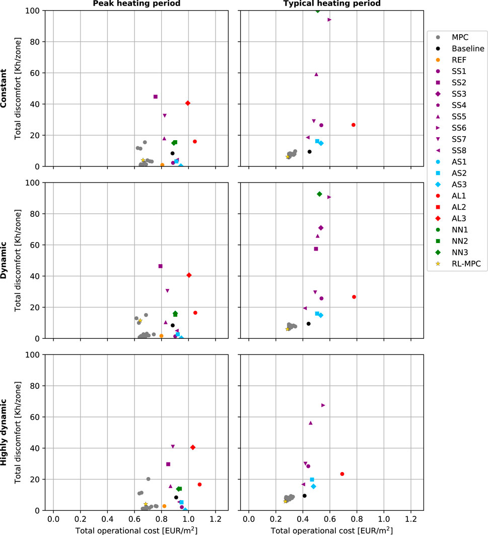
FIGURE 10. RL performance results for different test case runs in each of the BOPTEST scenarios. The rows show the results for the same pricing scenario, and the columns for the same period scenario. The results are obtained for different configurations of the state space, action space, learning algorithm, and neural network architecture.
What stands out from Figure 10 is that the performance results from the RL agents are more scattered than those obtained with MPC, which consistently outperforms both the baseline and the RL agents. None of the RL variants achieve the optimality level of the MPC or RL-MPC. The scale of Figure 10 has been limited for clarity leaving out a few cases like AL2 or AL3 during the typical heating period. In general, it is observed that the agents struggle more during the typical heating period because the effect of ambient temperature and solar irradiation is more prominent during this period. An example is the reference case that can achieve good comfort levels during the peak heating period but fails to meet comfort constraints during the typical heating period. A similar effect is observed for NN1, NN2, and NN3. Only the agents handling small state space dimensions from reduced prediction horizons or increased control step sizes like SS4, SS5, SS6, or SS7 appear all within the scale depicted in Figure 10, but most of the times, they do not show satisfactory performance levels.
It is worth noting that the variants implementing indirect control (AS2 and AS3) achieve low discomfort levels during the peak heating period but at a considerably higher operational cost compared to MPC. This emphasizes the larger potential for implementing direct control. Moreover, variants AS2 and AS3 increase their discomfort levels during the typical heating period because this period requires a more accurate control strategy taking care of disturbances to avoid overheating.
Contrary to the cases commented above, RL-MPC shows an excellent control performance during the typical heating period. Specifically, RL-MPC performs as well as the best MPC from all MPC variants during the typical heating period, and similarly to the general MPC results during the peak heating period. The outstanding performance during the typical heating period indicates that the value function can incorporate the effect of the weather conditions, i.e., of the ambient temperature and solar irradiation.
The main differences between the computational cost of the implemented algorithms relate to their offline and online computational needs. RL has a high offline computational demand because the algorithms need to interact with the building environment for several episodes of experience during the training process. Once the policy or the value function has been trained, the online computational demand of RL agents is very low because calculating the control action only comes at the cost of a function evaluation. On the contrary, MPC requires almost no offline computation but has a higher online computational demand. The reason is that an optimization problem needs to be solved every control step. RL-MPC has an equivalent offline computational demand as the one of RL since it also needs a value function to be trained beforehand, and an online computational demand as the one of MPC since it also needs an optimization to be solved every control step. In the latter case, however, the optimization is truncated along the prediction horizon with the value function, which eases the solution of the associated non-linear program.
One of the core KPIs provided by BOPTEST is the computational time ratio, which calculates the average ratio between the controller computation time and the test simulation control step period. More specifically, the computational time ratio κtimr is calculated as
where K is the set of all control steps, Δtc,k is the elapsed controller computational time at step k, and Δts,k is the interval of control step k. This ratio indicates the remaining time that a controller has to compute a control action every control step. The ratio has been collected for all controllers in this study. The RL agents show a computational time ratio in the order of
The use of RL for BEM is appealing because of its model-free approach and its learning capabilities. Many studies have investigated the use of RL for BEM e.g., for their application in DR settings. However, reduced order models are used to test the effectiveness of their RL algorithms and they claim that performance improvements can be attained with the model-free approach. The work presented in this paper has shown a different reality when implementing RL for direct building climate control in a reliable building emulator from the BOPTEST framework. Despite using state-of-the-art RL algorithms and the same environment for learning and testing, the RL agents seriously struggle to perform well in an environment characterized by realistic building dynamics. Variations in the learning algorithms and their hyperparameters have been explored, but they generally score worse than the consistently performant results of the MPC approach.
It has been shown that indirect control leads to a safer operation within the constraints set but limits the performance potential of an agent. Hence, classical model-free RL is not a valid option for direct control of building systems. It is likely that the discrepancy between these findings and those from prior literature stems from the use of a detailed testing emulator with realistic building dynamics. RL algorithms are appropriate for learning environments with a clear causal relation between actions and rewards but fall short when learning environments where the causal relation is not as clear or is delayed in time (Dulac-Arnold et al., 2019). Reduced-order models simplify the dynamic coupling between actions and rewards which facilitates the agent’s learning. However, these simplifications should not be used for testing as the associated models are not representative of actual buildings.
RL may still serve in combination with model-based approaches using more sophisticated methods to combine operational safety and learning simultaneously. An example of this practice is the RL-MPC algorithm as proposed in (Arroyo et al., 2022). RL-MPC has shown similar performance results as those from MPC for all testing scenarios of the considered building case. However, these approaches require tuning from an expert so that their expert-free property cannot be claimed anymore. Perhaps further RL research leads to significantly sample efficient algorithms that can be directly implemented for direct climate control. However, the results of this paper indicate that we are not yet at that point.
A limitation of this work is that it lacks testing in multi-input building systems. RL agents are expected to be substantially more challenged in those cases since the curse of dimensionality compromises their scalability. The study conducted in this paper is also limited by a deterministic setting. RL techniques are expected to excel for those scenarios involving uncertainty, although they first need to prove their performance in a deterministic setting. Future research should compare these approaches in stochastic settings with regulated levels of uncertainty. It is expected that RL algorithms may improve their relative performance when compared to MPC in stochastic settings because RL methods can naturally learn the uncertainty of their environment. Standard MPC does not typically learn from its environment unless machine learning methods are implemented to mitigate the uncertainty associated with the forecast of the disturbances. In these cases, supervised learning algorithms can be used to estimate and correct the forecasted disturbances based on historical data, but the controller does not improve its control policy from rewards that are directly perceived from the environment. Furthermore, only a few hyperparameter settings have been explored from all those that could be investigated. Examples of other hyperparameters that should be considered for their evaluation in future research are the MPC transcription optimization techniques or the use of FQI RL techniques for direct building climate control. We hope that BOPTEST and BOPTEST-Gym will facilitate further exploration of different combinations of hyperparameter settings of optimal control.
This paper implements and compares MPC, RL, and RL-MPC for building control. MPC is implemented for different combinations of the prediction horizon and control step period. All MPC configurations outperform the baseline controller of the building except those with a prediction horizon period that is 12 times shorter than the time constant of the envisaged building. The BOPTEST-Gym interface is used to explore variations of the RL agents. Particularly, it is analyzed variations of their state-action space, learning algorithm and value function network architecture. From all tested variants of RL, most of them struggled to provide comfort during testing, and none of them was able to outperform the results of MPC for the same building case and testing scenarios. These results were found even when conditions favored the implementation of RL by letting the agent interact with the testing environment for substantial training periods. Letting the agents interact with the environment for prolonged time periods is unlikely in practice but reveals an upper performance bound of the RL algorithms when tested in a deterministic setting with a perfect model representation that has realistic dynamics.
From all hyperparameters explored, the learning algorithm had the highest effect on training and testing performance, indicating that off-policy algorithms are more suitable for the envisaged application. It is also shown that indirect control (a common practice when applying RL to buildings) offers safer operation but lowers the optimality potential of the controller.
Although the above conclusions are not very promising for applying model-free RL to direct building climate control, machine learning methods may still be helpful for this application, specially when combining these methods, e.g., as it is done in the RL-MPC algorithm that truncates the MPC objective function with a value function learned from using value-based RL methods.
The original contributions presented in the study are included in the article/Supplementary Material, further inquiries can be directed to the corresponding author.
JA: Conceptualization, Methodology, Software, Formal analysis, Data Curation, Writing–Original Draft, Writing–Review; Editing, Visualization, Funding acquisition FS: Conceptualization, Methodology, Writing-Review; Editing, Supervision, Funding acquisition LH: Conceptualization, Methodology, Writing–Review; Editing, Supervision, Funding acquisition.
This research is financed by VITO through a PhD Fellowship under the grant no. 1710754 and by KU Leuven through the C2 project Energy Positive Districts (C24M/21/021). This work emerged from the IBPSA Project 1, an international project conducted under the umbrella of the International Building Performance Simulation Association (IBPSA). Project 1 will develop and demonstrate a BIM/GIS and Modelica Framework for building and community energy system design and operation.
The authors declare that the research was conducted in the absence of any commercial or financial relationships that could be construed as a potential conflict of interest.
All claims expressed in this article are solely those of the authors and do not necessarily represent those of their affiliated organizations, or those of the publisher, the editors, and the reviewers. Any product that may be evaluated in this article, or claim that may be made by its manufacturer, is not guaranteed or endorsed by the publisher.
1This action space implements a backup controller
2This neural network implements normalization of the hidden layers
Abadi, M., Agarwal, A., Barham, P., Brevdo, E., Chen, Z., Citro, C., et al. (2015). TensorFlow: Large-Scale Machine Learning on Heterogeneous Systems. Software available from tensorflow.org. arXiv. Available at: https://arXiv.org/abs/1603.04467v2.
Andersson, J. A. E., Gillis, J., Horn, G., Rawlings, J. B., and Diehl, M. (2019). CasADi: a Software Framework for Nonlinear Optimization and Optimal Control. Math. Prog. Comp. 11, 1–36. doi:10.1007/s12532-018-0139-4
Arroyo, J., Manna, C., Spiessens, F., and Helsen, L. (2021). “An OpenAI-Gym Environment for the Building Optimization Testing (BOPTEST) Framework,” in Proceedings of the 17th IBPSA Conference (Belgium: Bruges).
Arroyo, J., Manna, C., Spiessens, F., and Helsen, L. (2022). Reinforced Model Predictive Control (RL-MPC) for Building Energy Management. Appl. Energ. 309 (2022), 118346. doi:10.1016/j.apenergy.2021.118346
Arroyo, J., van der Heijde, B., Spiessens, F., and Helsen, L. (2018). “A Python-Based Toolbox for Model Predictive Control Applied to Buildings,” in Proceedings of the 5th International High Performance Building Conference (Indiana, USA: West Lafayette).
Axelsson, M., Magnusson, F., and Henningsson, T. (2015). A Framework for Nonlinear Model Predictive Control in JModelica.Org. Proc. 11th Int. Modelica Conf. Versailles, France, September 118, 301–310. 21-23. doi:10.3384/ecp15118301
Blum, D., Arroyo, J., Huang, S., Drgoňa, J., Jorissen, F., Walnum, H. T., et al. (2021). Building Optimization Testing Framework (BOPTEST) for Simulation-Based Benchmarking of Control Strategies in Buildings. J. Building Perform. Simulation 14 (5), 586–610. doi:10.1080/19401493.2021.1986574
Chen, B., Cai, Z., and Bergés, M. (2019). “Gnu-RL: A Precocial Reinforcement Learning Solution for Building HVAC Control Using a Differentiable MPC Policy,” in Proceedings of the 6th ACM International Conference on Systems for Energy-Efficient Buildings, Cities, and Transportation (BuildSys) (New York, USA, 316–325.
De Coninck, R., Magnusson, F., Åkesson, J., and Helsen, L. (2016). Toolbox for Development and Validation of Grey-Box Building Models for Forecasting and Control. J. Building Perform. Simulation 9 (3), 288–303. doi:10.1080/19401493.2015.1046933
De Somer, O., Soares, A., Vanthournout, K., Spiessens, F., Kuijpers, T., and Vossen, K. (2017). “Using Reinforcement Learning for Demand Response of Domestic Hot Water Buffers: A Real-Life Demonstration,” in Proceedings of the IEEE PES Innovative Smart Grid Technologies Conference Europe (ISGT-Europe) (Turin, Italy, 1–7. doi:10.1109/isgteurope.2017.8260152
Drgoňa, J., Arroyo, J., Cupeiro Figueroa, I., Blum, D., Arendt, K., Kim, D., et al. (2020). All You Need to Know about Model Predictive Control for Buildings. Annu. Rev. Control. 50, 190–232. doi:10.1016/j.arcontrol.2020.09.001
Dulac-Arnold, G., Mankowitz, D., and Hester, T. (2019). Challenges of Real-World Reinforcement Learning. arXiv. Available at: https://arXiv.org/abs/1904.12901.
European CommissionDirectorate-General for EnergyEnergy prices and costs in europe (2020). Available at: https://eur-lex.europa.eu/legal-content/EN/TXT/?uri=CELEX:52016DC0769.
Haarnoja, T., Zhou, A., Abbeel, P., and Levine, S. (2018). Soft Actor-Critic: Off-Policy Maximum Entropy Deep Reinforcement Learning with a Stochastic Actor. arXiv. Available at: https://arxiv.org/abs/1801.01290.
Hill, A., Raffin, A., Ernestus, M., Gleave, A., Kanervisto, A., Traore, R., et al. (2018). Stable Baselines. Available at: https://github.com/hill-a/stable-baselines.
IEAGlobalABCUN Environmental Programme (2019). Global Status Report for Buildings and Construction: Towards a Zero-Emissions, Efficient and Resilient Buildings and Construction Sector. Tech. Rep. Available at: https://wedocs.unep.org/handle/20.500.11822/30950.
IEAGlobalABCUN Environmental Programme (2020). Global Status Report for Buildings and Construction: Towards a Zero-Emissions, Efficient and Resilient Buildings and Construction Sector. Tech. Rep. Available at: https://wedocs.unep.org/handle/20.500.11822/34572.
Jorissen, F., Reynders, G., Baetens, R., Picard, D., Saelens, D., and Helsen, L. (2018). Implementation and Verification of the IDEAS Building Energy Simulation Library. J. Building Perform. Simulation 11 (6), 669–688. doi:10.1080/19401493.2018.1428361
Liu, S., and Henze, G. P. (2006). Experimental Analysis of Simulated Reinforcement Learning Control for Active and Passive Building thermal Storage Inventory. Energy and Buildings 38 (2), 148–161. doi:10.1016/j.enbuild.2005.06.001
Mbuwir, B. V., Geysen, D., Spiessens, F., and Deconinck, G. (2019). Reinforcement Learning for Control of Flexibility Providers in a Residential Microgrid. IET Smart Grid 3 (98), 1–107. doi:10.1049/iet-stg.2019.0196
Mbuwir, B. V., Spiessens, F., and Deconinck, G. (2019). “Benchmarking Regression Methods for Function Approximation in Reinforcement Learning: Heat Pump Control,” in Proceedings of the IEEE PES Innovative Smart Grid Technologies Europe (ISGT-Europe) (Bucharest, Romania: September), 1–5. doi:10.1109/isgteurope.2019.8905533
Mnih, V., Badia, A. P., Mirza, M., Graves, A., Lillicrap, T. P., Harley, T., et al. (2016). Asynchronous Methods for Deep Reinforcement Learning. arXiv. Available at: https://arxiv.org/abs/1602.01783.
Mnih, V., Kavukcuoglu, K., Silver, D., Graves, A., Antonoglou, I., Wierstra, D., et al. (2013). Playing Atari with Deep Reinforcement Learning. arXiv. Available at: http://arxiv.org/abs/1312.5602.
Patyn, C., Ruelens, F., and Deconinck, G. (2018). “Comparing Neural Architectures for Demand Response through Model-free Reinforcement Learning for Heat Pump Control,” in Proceedings of the 2018 IEEE International Energy Conference (ENERGYCON) (Limassol, Cyprus).
Peirelinck, T., Ruelens, F., and Decnoninck, G. (2018). “Using Reinforcement Learning for Optimizing Heat Pump Control in a Building Model in Modelica,” in Proceedings of the IEEE International Energy Conference (Limassol, Cyprus: ENERGYCON), 1–6. doi:10.1109/energycon.2018.8398832
Picard, D., Drgoňa, J., Kvasnica, M., and Helsen, L. (2017). Impact of the Controller Model Complexity on Model Predictive Control Performance for Buildings. Energy and Buildings 152, 739–751. doi:10.1016/j.enbuild.2017.07.027
Ruelens, F., Claessens, B. J., Vandael, S., De Schutter, B., Babuška, R., and Belmans, R. (2017). Residential Demand Response of Thermostatically Controlled Loads Using Batch Reinforcement Learning. IEEE Trans. Smart Grid 8 (5), 2149–2159. doi:10.1109/TSG.2016.2517211
Ruelens, F., Claessens, B. J., Vrancx, P., Spiessens, F., and Deconinck, G. (2019). Direct Load Control of Thermostatically Controlled Loads Based on Sparse Observations Using Deep Reinforcement Learning. arXiv. Available at: https://arxiv.org/abs/10.17775/CSEEJPES.2019.00590.
Schulman, J., Wolski, F., Dhariwal, P., Radford, A., and Klimov, O. (2017). Proximal Policy Optimization Algorithms. Available at: https://arxiv.org/abs/1707.06347.
Sun, F., Li, G., and Wang, J. (2009). “Unscented Kalman Filter Using Augmented State in the Presence of Additive Noise,” in Proceedings of the IITA International Conference on Control, Automation and Systems Engineering (China: Zhangjiajie), 379–382. doi:10.1109/case.2009.51
Sutton, R. S., and Barto, A. G. (2018). Reinforcement Learning: An Introduction. second ed. The MIT Press.
Touzani, S., Prakash, A. K., Wang, Z., Agarwal, S., Pritoni, M., Kiran, M., et al. (2021). Controlling Distributed Energy Resources via Deep Reinforcement Learning for Load Flexibility and Energy Efficiency. Appl. Energ. 304 (2021), 117733. doi:10.1016/j.apenergy.2021.117733
van Hasselt, H., Guez, A., and Silver, D. (2015). Deep Reinforcement Learning with Double Q-Learning. arXiv. Available at: http://arxiv.org/abs/1509.06461.
Wan, E. A., and Van Der Merwe, R. (2000). “The Unscented Kalman Filter for Nonlinear Estimation,” in IEEE 2000 Adaptive Systems for Signal Processing, Communications, and Control Symposium (Lake Louise, AB, Canada: AS-SPCC 2000), 153–158. doi:10.1109/ASSPCC.2000.882463
Zhang, Z., and Lam, K. (2018). “Practical Implementation and Evaluation of Deep Reinforcement Learning Control for a Radiant Heating System,” in Proceedings of the 5th ACM International Conference on Systems for Energy-Efficient Buildings, Cities, and Transportation (BuildSys) (China: Shenzen), 148–157. doi:10.1145/3276774.3276775
Keywords: model predictive control, reinforcement learning, building modeling, thermal management, optimization, artificial neural network
Citation: Arroyo J, Spiessens F and Helsen L (2022) Comparison of Optimal Control Techniques for Building Energy Management. Front. Built Environ. 8:849754. doi: 10.3389/fbuil.2022.849754
Received: 06 January 2022; Accepted: 21 February 2022;
Published: 01 April 2022.
Edited by:
Jacopo Vivian, Swiss Federal Laboratories for Materials Science and Technology, SwitzerlandCopyright © 2022 Arroyo, Spiessens and Helsen. This is an open-access article distributed under the terms of the Creative Commons Attribution License (CC BY). The use, distribution or reproduction in other forums is permitted, provided the original author(s) and the copyright owner(s) are credited and that the original publication in this journal is cited, in accordance with accepted academic practice. No use, distribution or reproduction is permitted which does not comply with these terms.
*Correspondence: Javier Arroyo, amF2aWVyLmFycm95b0BrdWxldXZlbi5iZQ==
Disclaimer: All claims expressed in this article are solely those of the authors and do not necessarily represent those of their affiliated organizations, or those of the publisher, the editors and the reviewers. Any product that may be evaluated in this article or claim that may be made by its manufacturer is not guaranteed or endorsed by the publisher.
Research integrity at Frontiers
Learn more about the work of our research integrity team to safeguard the quality of each article we publish.