Probabilistic Fatigue Fragility Curves for Overhead Transmission Line Conductor-Clamp Assemblies

The residual life of transmission line overhead conductors under conditions of fretting fatigue is an important asset management issue for electric network operators. The current industry practice for overhead conductor residual life estimation relies heavily on experimentally generated fatigue curves or rule-based expert systems. The current experiment-based methods do not consider specific conductor-clamp configurations and are based on the simple flexion model. This approach results in large uncertainties in service life predictions and are limited to a failure criterion based on the first wire failure in the conductor. Rule-based expert systems also have limited applicability since they lack physical representation of the fretting fatigue process. Given the limitations of the current methods, the objective of this work is to propose a framework that combines physics-based models and probability theory to estimate the residual life of overhead conductors considering either single or multiple wire failure criteria. To illustrate this procedure, a finite element model of a Bersfort conductor-clamp system is used to assess the contact conditions and internal stress states in the wires of the conductor. Results from the numerical model are then used to develop a fretting fatigue criterion that is a function of the contact energy dissipation mechanisms, contact stresses, and the plain fatigue resistance of the wires. Probability of failure of each contact point between wires and between wires and clamp is computed using the fretting fatigue criterion. With this information, the most probable locations of fretting fatigue failure are identified in the conductor. The predictions for the locations of failure are validated with available literature data for the same conductor-clamp configuration. Given the probabilities of failures at each contact point, the probability of failure of the conductor is derived with the Poisson binomial distribution. Fragility curves are presented for the first through the third wire failures in the conductor. The fragility curves are validated through comparisons with available literature data on the same conductor-clamp configuration. Fatigue curves are also generated from the fragility model for the first wire failure and compared against experimentally generated fatigue curves.

Introduction

Aging of infrastructure coupled with a projected increased reliance on electric energy has been an issue of concern for electrical utilities worldwide. Overhead conductors are the major components of a transmission line network, and there has been an increased interest in estimating the residual life of the overhead conductors for improving asset management planning (Hathout, 2016; Pouliot et al., 2020). The dominant mechanisms associated with the degradation of overhead transmission line conductors are atmospheric corrosion and fretting fatigue. Among these two phenomena, fretting fatigue has received the most attention.

For conductor-clamp assemblies, field observation has shown that fretting fatigue is caused by aeolian vibrations that induce cyclic bending of the conductor and that fatigue damage is confined to the clamp/keeper where the conductor is supported (CIGRE 2010; Cloutier et al., 2006; Rawlins, 1979) (Figure 1). The cyclic motion of the conductor causes relative motions at wire-to-wire, wire-to-clamp, and wire-to-keeper contacts (Cloutier et al., 2006). The relative motion at contacts leads to the phenomenon of fretting, which is a surface degradation process that leads to the formation of surface cracks (Hills and Nowell, 1994). In the presence of tension (Hills and Nowell, 1994) and bending moment (Lalonde et al, 2018) in the wires, the surface cracks propagate through the wire leading to fretting fatigue failure.

FIGURE 1

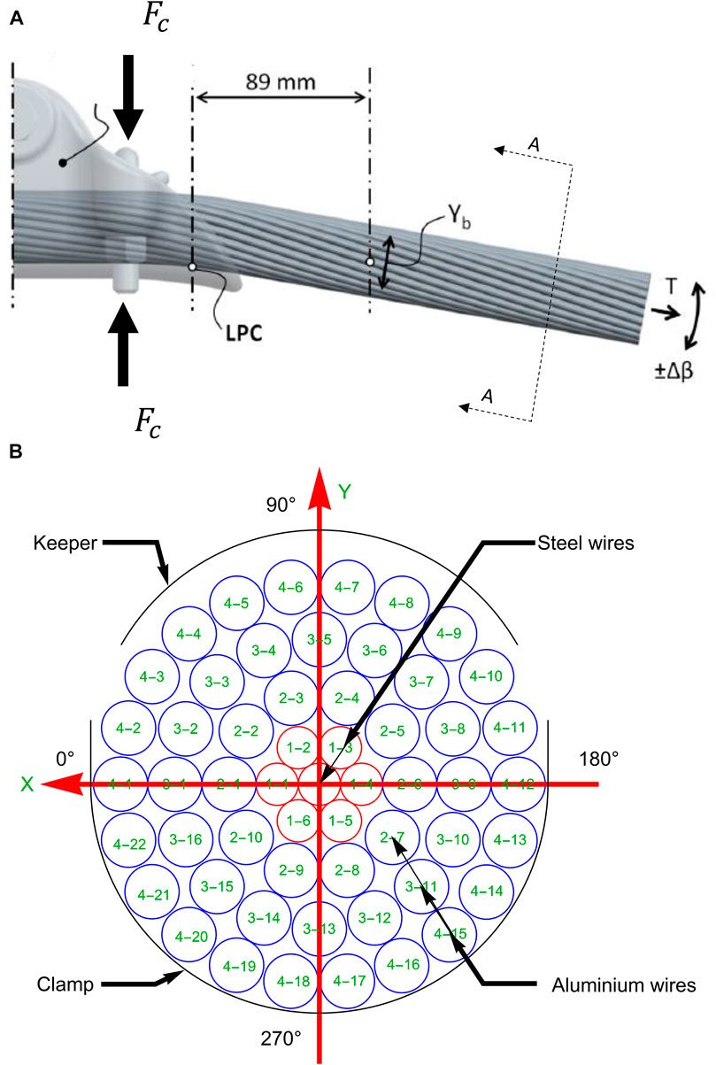
FIGURE 1. (A) Typical conductor-clamp assembly with applied conductor tension (T), clamping force (F_C), change in alternating bending angle (Δβ), and bending amplitude (Yb) [adapted from Lalonde et al. (2018)]. (B) Cross-section A-A of a typical conductor-clamp assembly showing the steel wires, aluminum wires, keeper and clamp configuration, and the wire numbering system.

Simplified analytical models have been developed to relate the bending amplitude ($Y_b$) of vibration of the conductor at a specified distance from the last point of contact (LPC) with the clamp, to an idealized stress measure ${\sigma }_a$ at the topmost fiber of the conductor at the LPC (Figures 1A, 2) (Poffenberger and Swart, 1965). The idealized bending stress is defined in Lalonde et al. (2017) as:

${\sigma }_a=\frac{d_c E_a \left(\frac{T}{4 EI}\right)}{e^{-\sqrt{T/EI} z }-1 + \sqrt{T/EI} z }{Y}_b(1)$

FIGURE 2

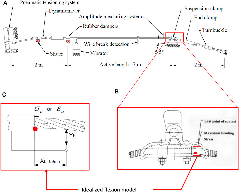
FIGURE 2. (A) Fatigue testing bench for conductor-clamp systems [adapted from (CIGRE, 2010)]. (B) Conductor-clamp assembly showing region of maximum bending stress (Cloutier and Lalonde, 2007). (C) Simplified representation of the conductor-clamp assembly and the idealized stress or strain induced by bending amplitude Y_b (Cloutier and Lalonde, 2007).

where $d_c$ is the diameter of the conductor, $E_a$ is the modulus of elasticity of aluminum, T is the tension applied to the conductor, $Y_b$ is the bending amplitude at 89 mm from the last point of contact as shown in Figure 1A, and $EI$ is the bending stiffness of the conductor defined in Cloutier et al. (2006) as:

$EI={\displaystyle \sum _{i=1}^{number of wires }}{E}_i I_i(2)$

where $E_i$ and $I_i$ are the Young modulus and moment of inertia of the ith wire. The idealized stress obtained from Equation 1 is derived under the assumption that the conductor wires act independently in the region where the conductor enters the clamp, and is modeled as a Euler-Bernoulli beam with a fixed end (Figures 2B, C) (Cloutier et al., 2006).

Based on the idealized stress model, experimental fatigue test benches, such as that shown in Figure 2A, are used to obtain experimental stress-number of cycles data $\left\{{\sigma }_a,Number of cycles\right\}$ for various conductor-clamp assemblies (Cardou and Cloutier, 1990; CIGRE, 1979; Cloutier et al., 2006). Compilations of these experimental datasets have been used to derive empirical Stress-Number of cycles (SN) curves to predict first wire failures in conductors (Cloutier et al., 2006; Rawlins, 1979; CIGRE, 1979; Hardy and Leblond, 2001; and; Thomas et al., 2020). However, SN models derived from experimental test benches that rely on the idealized bending model have limited applicability due to the reliance on the idealized stress, which neglects effects associated with the clamping force and clamp/keeper. Another limitation from compiled databases is the lack of uniform testing protocols between laboratories. Finally, the tests are very expensive and time-consuming to perform, and the resulting SN curves are usually valid only for the first wire failure in the conductor.

In order to derive SN curves for multiple wire failures, Lalonde et al. (2017) modeled a conductor using 3D beam elements. However, this work did not model the clamp/keeper of conductor/clamp assembly but only the conductor was modeled, and it was assumed that the clamp/keeper can be replaced by fixed end boundary conditions. The stresses developed at the fixed end are then used to determine the number of cycles to failure from plain wire fatigue data from which first wire failure SN curves were developed. The limitation of this work is the simplification of the clamp/keeper as a fixed end boundary condition and its inability to account for the possibility of failure at multiple locations within a conductor-clamp assembly.

Models have also been proposed that focus on a single critical location for wire failure and do not account for the possibility of failure at multiple locations within the conductor-clamp assembly (Said et al., 2020; Omrani et al., 2021). In Omrani et al. (2021), a numerical model of the conductor-clamp assembly is used to identify the wire and contact with the largest contact stresses, which is assumed to be the location for the first wire failure. The state of stress obtained from the numerical model for different amplitudes of vibration is used to specify loads to be applied in single wire fretting fatigue experiments and to develop a (first-wire failure) SN curve for the conductor-clamp assembly. However, results from these single contact experiments overestimate the number of cycles at which first wire failures are observed experimentally for conductor-clamp assemblies with multiple wire–wire and wire–clamps contacts.

Considering the limitations of current models, the objective of this work is to propose a framework that combines the physically based numerical model of Lalonde et al. (2018), single wire plain fatigue data, and probabilistic models to estimate fragility and SN curves that can account for multiple contacts and multiple wire failures within conductor-clamp assemblies. To achieve this, the finite element model of Lalonde et al. (2018) for a Bersfort conductor is used to assess the fretting regimes and internal stresses at each contact. A fatigue criterion is proposed that considers the fretting regimes, internal stresses, and the plain fatigue strength of the constituent wires of the conductor. The fatigue criterion is used to rank contacts for fatigue failure and to estimate the probability of failure from plain fatigue data for a given amplitude and number of cycles. Surfaces representing the probabilities of failure of each layer in the Bersfort conductor are generated for varying numbers of cycles and bending amplitude. The Poisson Binomial distribution is then used to generate fragility curves that consider different probabilities of failure at each contact point and wire-to-wire variability in fatigue resistance, which gives fatigue life predictions for one or multiple wire failures (up to 3 in this application). The fragility curves are compared to empirical cumulative distribution functions derived from experimental data for the same conductor-clamp configuration (Levesque, 2005). The probability distribution for the number of failed wires as a function of the number of cycles is also obtained. SN curves generated from the new approach for first wire failures are also presented for the specimen conductor-clamp configuration and compared against the current available SN curves.

The Finite Element Modeling Methodology

A finite element model is used to reproduce the conditions of the experimental fatigue test bench used by Levesque (2005) (Figure 2). The model follows the procedure of Lalonde et al. (2018), which uses quadratic 3D Timoshenko beam elements (10 mm in length) for the wires, and quadratic rigid shell elements (2.5 mm in length and width) for the clamp and keeper. The wire–wire, and wire–clamp/keeper contacts are modeled using line-to-line and line-to-surface contact elements in the ANSYS^® system. Lalonde et al. (2018) have demonstrated that the beam model can accurately reproduce the strains measured experimentally in the wires of the Bersfort conductor-clamp assembly.

In this work, the conductor-clamp assembly modeled is a Bersfort conductor-clamp as shown in Figure 3. A cross-section of the conductor is shown in Figure 1B and the length of the conductor is 1,600 mm. Additional geometric details on the conductor-clamp assembly can be found in Lalonde et al. (2018) and Goudreau et al. (2010). The finite element mesh of the conductor-clamp assembly and contact elements are shown in Figure 4.

FIGURE 3

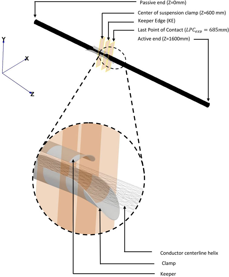
FIGURE 3. Geometric representation of the Bersfort conductor-clamp system.

FIGURE 4

FIGURE 4. (A) Finite element mesh of the Bersfort conductor-clamp assembly showing the beam and rigid shell elements. (B) Line-to-line contact between the conductor wires of the same layers modeled with slave element CONTA177 and master element TARGE170. (C) Line-to-line contact between the conductor wires of different layers modeled with slave element CONTA177 and master element TARGE170. (D) Line-to-surface contact between the layer 4 wires and the keeper/clamp.

The material properties of the conductor wires are listed in Table 1. The core is a steel wire in the center of the conductor (Figure 1B). The layer numbering and wire numbering are also shown in Figure 1B. The coefficient of friction is 0.3 for steel-to-steel contacts and 0.9 for aluminum-to-aluminum and aluminum-to-steel contacts (Lalonde et al., 2018; Omrani et al., 2021).

TABLE 1

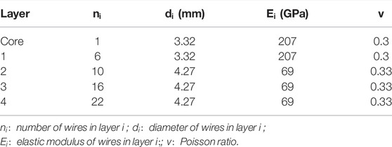
TABLE 1. Characteristics of the Bersfort conductor (Lalonde et al., 2018).

The beams are modeled as linear elastic elements with large displacement and rotation capabilities. The linear elastic assumption has been shown to provide fretting fatigue life predictions for aluminum wires that are in agreement with experimental fatigue life observations (Rocha et al., 2019; Said et al., 2020).

Load Application and Sequencing Scheme

The loading sequence of the Bersfort conductor finite element model follows the experimental procedure established in Levesque (2005) who tested Bersfort conductors with the fatigue test bench shown in Figure 2, and is similar to the sequence used by Lalonde et al. (2018) in their numerical model. For the load application to the model, the nodes of the beams at the passive end of the conductor are coupled to a master node located at the center of the conductor using Multiple Point Constraints (MPC) (Figure 5). The nodes of beams at the active end (Figure 5) are similarly coupled to a master node at the center of the conductor. For the clamp/keeper, all the nodes are coupled using rigid MPC. For the clamp, all nodal degrees of freedom (DOF) are fixed for displacements and rotations. For the keeper, all rotation and displacement are fixed except for the displacement in the y-direction.

FIGURE 5

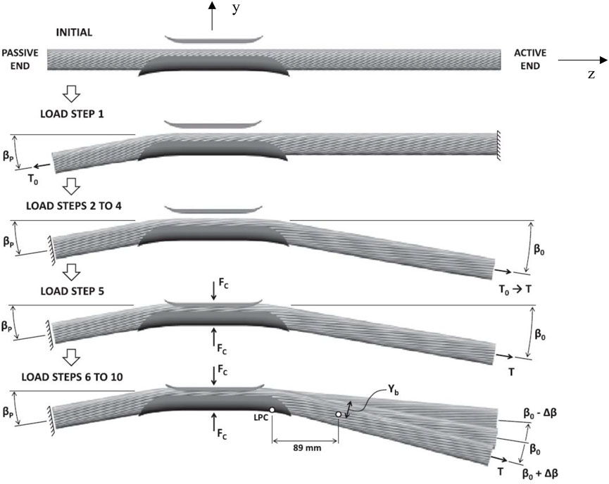
FIGURE 5. Loading sequence of the Bersfort conductor-clamp assembly [adapted from Lalonde et al. (2018)].

The first step of the loading protocol is to incrementally apply an initial tension $T_0$ at the passive end of the conductor at an angle ${\beta }_p$ relative to the horizontal while the active end of the conductor is restrained for all 6 DOFs (Figure 5). At the end of step 1, the passive end is fixed at its current position and the z-direction and y-direction displacement DOF at the active end is released; this is followed by the application of the conductor tension $T_0$ at the master node of the active end at an angle ${\beta }_0$ (step 2 in Figure 5). During the loading steps 3 and 4, the conductor tension at the active end is increased from $T_0$ to $T$. The effect of the clamping force is simulated by introducing a force $F_c$ in the y-direction on the keeper master node in loading step 5. Once the clamping force is completely applied, it is replaced by the displacement induced by $F_c$. The loading steps 6 to 10 consist in cycling the angle of the active end of the conductor with tension T by $\pm \mathrm{\Delta }\beta$ to induce a displacement $Y_b$. The value of $\pm \mathrm{\Delta }\beta$ is specified to match the target bending amplitude $Y_b$. The loads and angles corresponding to the experimental setup are provided in Table 2. Additional details can be found in Lalonde et al. (2018) and Levesque (2005).

TABLE 2

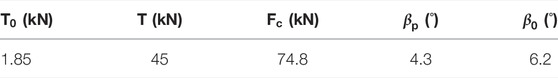
TABLE 2. Applied boundary conditions in finite element model (Lalonde et al., 2018).

Conductor Fatigue Model

Model Formulation

Fretting fatigue analysis for a single contact can be performed by specifying displacement and force boundary conditions on the two bodies in contact, a plain fatigue model, and a procedure to define an equivalent stress state that is related to the fretting fatigue potential. This approach has been followed by Redford et al. (2019) and Rocha et al. (2019) in the assessment of fretting fatigue failure for a wire/clamp and two wires in contact at a single contact point. However, for a multiple contacts system such as a conductor, it has been shown that contacts are subjected to at least three different fretting regimes—sticking regime, mixed fretting regime, and gross slip regime (Zhou and Vincent, 1995) and that the analysis must first determine if a contact is in a fretting regime that leads to crack initiation and propagation. This state introduces an additional criterion for the analysis of conductor fatigue in comparison to single contact fretting fatigue.

In the proposed methodology, a criterion is proposed that considers both the tangential force Q(t) and sliding distance $u\left(t\right)$. This criterion is based on the energy dissipated E at the contact and is given by:

$E={\displaystyle \oint Q\left(t\right)u\left(t\right)dt}(3)$

Where t is a time tracking parameter. A plot of $Q\left(t\right)$ against u(t) illustrates the various fretting regimes (Figure 6). In these figures, the axial position of contacts is:

$\mathrm{Axial\; position} = \mathrm{z\; coordinate} - LP{C}_{\mathit{exp}}(4)$

where $LP{C}_{exp}=685\text{mm}$ and is the last point of contact determined by Levesque (2005). A negative value of the axial position indicates that the contact is within the clamp while a positive value indicates that the contact is outside the clamp.

FIGURE 6

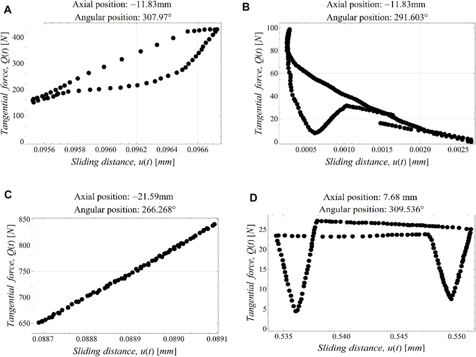
FIGURE 6. Examples of fretting regimes indicated by the plot of Q(t) against u(t) when the conductor goes through β₀ ± Δβ for a bending amplitude of 0.75 mm. (A) Mixed fretting regime on a layer 4 to layer 3 contact. (B) Mixed fretting regime on a layer 4 to clamp contact. (C) Sticking contact on a layer 4 to layer 3 contact. (D) Gross slip contact on a layer 4 to contact.

The three fretting regimes, sticking, mixed fretting, and gross slip, as defined by Zhou and Vincent (1995) are shown in Figure 6. The fretting regimes are defined by the energy dissipation curves for contacts between wire-to-wire and wire-to-clamp in conductor-clamp assemblies. The characteristic behaviors of the energy dissipation curves of these fretting regimes are given in Degat et al. (1997) and summarized as follows: The mixed fretting regime has a closed energy dissipation curve of elliptical shape, small or large tangential force, and short sliding distance (Figures 6A, B). The sticking regime is characterized by a closed loop energy dissipation curve in the shape of a line and large tangential force (Figure 6C). The gross slip is characterized by an open energy dissipation curve (often rectangular), small tangential force, and large sliding distance (Figure 6D).

The fretting regime is combined with the stress-based Smith-Watson-Topper (SWT) criteria to formulate the conductor fatigue criteria as:

$G\left(E\right) \left(SW{T}_L | Y_b=y\right)\ge \left(SW{T}_R | N=N_i\right)(5)$

where $SW{T}_L | y_b$ represents the Smith-Watson-Topper criteria of the wire contact at a given bending amplitude, and the SWT is defined in Rocha et al. (2019) as:

$SWT = \sqrt{\frac{\mathrm{\Delta }\sigma }{2}\langle {\sigma }_{\mathit{max}}\rangle }(6)$

where $\frac{\mathrm{\Delta }\sigma }{2}$ is the stress amplitude and ${\sigma }_{max}$ is the maximum stress in a loading cycle. The SWT is a tension-based fatigue criterion. From the 3D beam model, the stress range $\mathrm{\Delta }\sigma$ and maximum stress ${\sigma }_{max}$ are obtained as:

$\mathrm{\Delta }\sigma =\left|{\sigma }_1\left({\beta }_0+\mathrm{\Delta }\beta \right)-{\sigma }_1\left({\beta }_0-\mathrm{\Delta }\beta \right)\right|(7)$

${\sigma }_{\mathit{max}}=\max \left({\sigma }_1\left({\beta }_0+\mathrm{\Delta }\beta \right),{\sigma }_1\left({\beta }_0-\mathrm{\Delta }\beta \right)\right)(8)$

where ${\sigma }_1$ is the maximum principal stress at the beam nodes.

The values of ${\sigma }_1\left({\beta }_0+\mathrm{\Delta }\beta \right)and{\sigma }_1\left({\beta }_0+\mathrm{\Delta }\beta \right)$ obtained from the FE analysis are shown in Figure 7 for a bending amplitude of 0.75 mm for different wires (layers) in the Bersfort conductor-clamp assembly.

FIGURE 7

FIGURE 7. Distribution of maximum principal stresses (in MPa) for a bending amplitude of 0.75 mm. (A,C,E) β₀ + Δβ and (B,D,F) β₀ − Δβ.

In the following section, the fatigue resistance of a wire to plain fatigue for a given number of cycles N_i is defined through the Smith-Watson-Topper criteria $\left(SW{T}_R | N=N_i\right)$ and is estimated from rotating bending data provided in Kaufman (2008) for aluminum wires. A Basquin-type stress–life relationship is used to describe $SW{T}_R | N=N_i$, and it is assumed that $f_{SW{T}_R}\left(SW{T}_R | N=N_i\right)$ follows a lognormal distribution with mean $\mu \left(SWT\right)$ and standard deviation $\sigma \left(SWT\right)$, which are defined as (Pascual and Meeker, 1997; Babuška et al., 2016):

$\mu \left(SW{T}_R\right)=A_1+A_2\mathit{log}\left(SW{T}_R - A_3\right)(9)$

$\sigma \left(SW{T}_R\right)=\mathit{exp}\left(B_1 + B_2 \mathit{log}\left(SW{T}_R \right)\right)(10)$

where $f_{SW{T}_R}(.)$ is the probability distribution function. The parameter vector of the model $\mathit{\theta }=\left(A_1,A_2,A_3,B_1 ,B_2 \right)$ is estimated by the method of maximizing likelihood $\left(A_1=48.04,A_2=-7.37,A_3=2.23,B_1=5.46,B_2=-1.29\right)$ (Figure 8). The function G(E) defines the type of fretting regime as:

$G\left(E\right)=\{\begin{array}{cc}0& sticking regime\\ 1& mixed fretting regime\\ 0& gross slip regime\\ 0& no contact\end{array}(11)$

FIGURE 8

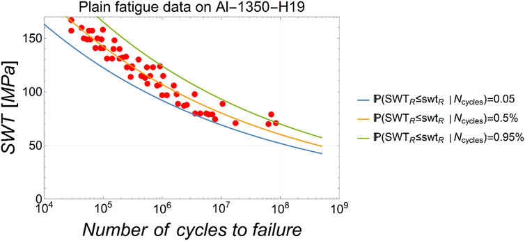
FIGURE 8. Fatigue data obtained from Kaufman (2008) and the fitted fatigue model.

This indicator function follows from experimental observations that the mixed fretting regime is the most critical for fretting fatigue in conductors (Zhou and Vincent, 1995). This function excludes other contacts that are not in this regime from the analysis. The value of $E$ for which a contact transitions from one regime to another is difficult to define precisely and relies on heuristics, such as the shape of hysteresis curve to assign values to $G\left(E\right)$ (Figure 6). Ideally, all types fretting regimes should be considered. Both the sticking and gross slip regimes can lead to crack initiation as shown in Zhou and Vincent (1995); however, the cracks do not propagate in the gross slip regime and do not lead to fatigue failure. In the case of the sticking regime, cracks can propagate to failure but typically this occurs for a number of cycles much larger than for the mixed fretting regime and can be ignored for a failure criterion based on a small number (<4) of wire failures.

In the following, only contacts between wires of different layers or between wires and the suspension clamp are considered for fretting fatigue. Contacts between wires on the same layer have much lower normal and tangential forces and are much less likely to be locations for the initiation and propagation of fretting fatigue failure. Considering the two contacts at the top and bottom of a wire segment discretized with a beam element m, the probability of failure of the wire segment for $N_i$ cycles at an amplitude y_b is:

${\mathbb{P}}_m\left(N=N_i\right)=\mathbb{P}\left(G\left(E_m\right) \left(SW{T}_{L_m}|y_b\right)\ge \left(SW{T}_R|N=N_i\right)\right)(12)$

The probability of failure of k wires within the conductor-clamp assembly can then be expressed as:

$\mathbb{P}\left(k|N=N_i\right)={\displaystyle \sum _{A \in {\mathcal{G}}_k}{\displaystyle \prod _{t \in A}{\mathbb{P}}_m\left(N=N_i\right)}{\displaystyle \prod _{j \in A^c}\left(1-{\mathbb{P}}_m\left(N=N_i\right)\right)}}(13)$

where ${\mathcal{G}}_k$ is the set of size $\left(\begin{array}{c}n\\ k\end{array}\right)$ of all combinations of k failed wires that can be formed from the set of n contact points within the conductor/clamp assembly, A is the set of contact points where fretting fatigue failure occurs, t are members of A, $A^{\mathrm{\complement }}$ is the set of contacts points that do not fail in fretting fatigue, and j are members of $A^{\mathrm{\complement }}$. This equation is the Poisson binomial distribution described in Wang (1993) and provides the probability of obtaining exactly k wire failures at a given number of cycles. The failure of a conductor can then be defined as the first wire failure or by specifying the number of multiple wire failures. Assuming that failure of a conductor is defined when k (or more) wires have failed, the probability of failure of the conductor is evaluated as,

$\mathbb{P}\left(K\ge k|N=N_i\right)=1-\mathbb{P}\left(K<k|N=N_i\right)(14)$

Equation 14 considers both the top and bottom contacts acting on a wire segment. For 3D beam finite elements, the maximum principal stress ${\sigma }_1$ occurs at either the top or bottom contact since bending stresses predominate as shown by Lalonde et al. (2018). In consequence, only the contact with the maximal principal stress is considered in Equations 13, 14.

Since the finite element model is formulated for a specific position of the cable in contact with the clamp, contact points are spaced at 10-mm intervals in the axial direction and the angular position at 16° intervals as shown by the black dots in Figure 7. The results from experimental tests can correspond to locations of contacts that vary within this range. Since analyses cannot be performed to reproduce the exact conductor-clamp configuration of each experiment, a procedure based on interpolating the $SW{T}_L | y_b$ is used instead. The interpolation procedure averages stresses locally as a function of axial position d and angular position $\theta$ through a Gaussian kernel function with parameters ${\sigma }_d, {\sigma }_{\theta }$ as:

$\stackrel{smoothened}{\overbrace{SW{T}_L|y_b\left(d,\theta \right)}}={\displaystyle \sum _{j=1}^{n_{nodes}}k\left({\sigma }_d, {\sigma }_{\theta }\right)\cdot SW{T}_L|y_b\left(d_j,{\theta }_j \right)}(15)$

$k\left({\sigma }_d, {\sigma }_{\theta }\right)=\frac{1}{{\sigma }_d\sqrt{2 \pi }}{e}^{-{\left(\frac{d-d_j}{{\sigma }_d}\right)}^2 }\cdot \frac{1}{{\sigma }_{\theta }\sqrt{2 \pi }}{e}^{-{\left(\frac{\theta -{\theta }_j}{{\sigma }_{\theta }}\right)}^2 }(16)$

where $n_{nodes}$ is the number of nodes from which the maximum principal stresses are extracted from the finite element model; $d_j$ and ${\theta }_j$ are the axial and angular positions of the node j.

The estimates of ${\sigma }_d$ and ${\sigma }_{\theta }$ are obtained by maximizing the likelihood of the observed failures given the number of cycles and location of failure:

$l\left({\sigma }_d,{\sigma }_{\theta }\right)={\displaystyle \prod _{j=1}^{n_{failed wires}}{f}_{SW{T}_R|Y_b,{\sigma }_d,{\sigma }_{\theta },d_j,{\theta }_j}\left(SW{T}_L\left(Y_b,{\sigma }_d,{\sigma }_{\theta },d_j,{\theta }_j\right)|N_j\right)}(17)$

where $l\left({\sigma }_d, {\sigma }_{\theta }\right)$ is the likelihood function, $SWT\left(Y_b,{\sigma }_d,{\sigma }_{\theta },d_j,{\theta }_j\right)$ is obtained from Eq. 6, $n_{failed wires}$ is the set of observed first wire failures given $Y_b$ (0.75 and 0.6 mm), ($d_j,{\theta }_j$) is the position of the failure wire, N_j the number of cycles at failure, and $f_{SW{T}_R}$ is the probability distribution of SWT from plain fatigue wire data given failure occurs at N cycles (Eqs 9, 10).

Procedure for the Derivation of Fragility Curves

This section summarizes the steps in the procedure for deriving fragility curves (Figure 9). First, the finite element model of the conductor-clamp assembly is formulated in ANSYS finite element program. In step 2, the maximum principal stress at the top or bottom contact of each wire element is obtained. In step 3, the tangential force and sliding distance at the contact with the maximum principal stress are obtained from the FE model to define the fretting regime (Figure 6). This is followed by step 4, where $SW{T}_L | y_b$ is evaluated using Eq. 6. Step 5 involves averaging the $SW{T}_L|y_b$ values using Eq. 15 to obtain $\stackrel{smoothened}{\overbrace{SW{T}_L|y_b\left(d,\theta \right)}}$. The indicator function G(E) (Eq. 11) is assigned to each node as a function of the corresponding fretting regime in step 6. Step 7 consists in fitting the fatigue model (Eqs 9, 10) to the plain fatigue data (Figure 8) to obtain $f_{SW{T}_R}\left(SW{T}_R | N=N_i\right)$. In step 8, the indicator function G(E) and the $\stackrel{smoothened}{\overbrace{SW{T}_L|y_b\left(d,\theta \right)}}$ are used to obtain the probability of failure for each beam element (Eq. 12). Finally, in step 9, the probability of k wire failures in the conductor is computed using the Poisson binomial distribution given by Eqs 13, 14.

FIGURE 9

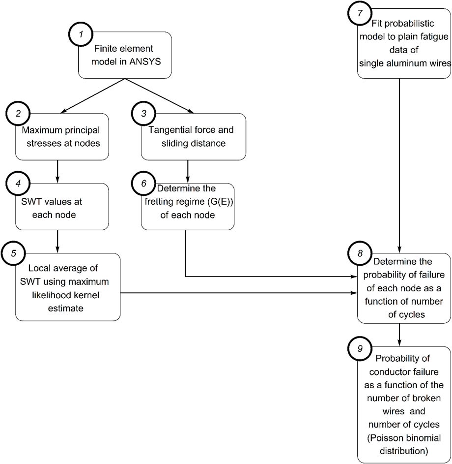
FIGURE 9. Flow chart for developing conductor-clamp assembly fragility curve.

The procedure from step 8 to step 9 is repeated to evaluate the probability of failure for the desired range of number of cycles (${10}^4$–${10}^7$).

Model Validation and Discussion

Validation of the framework is done by first comparing the predicted $\stackrel{smoothened}{\overbrace{SW{T}_L|y_b\left(d,\theta \right)}}$ and indicator function G(E) from the FE model to observed failure locations reported in Levesque (2005). Next, the empirical cumulative distribution function (ECDF) of the fatigue life for a given number of wire failure is compared against the predicted cumulative distribution function (CDF) generated by the Poisson binomial distribution given in Eq. 14.

For bending amplitudes of 0.75 mm, only 13 of the experiments report the location, order of wire failure, and number of cycles to failure (39 events for first to third wire failures), while 15 experiments report the same for an amplitude 0.60 mm. Two additional experiments providing the first wire failure for bending amplitudes of 0.4 and 0.5 mm are also available.

In application of the framework, the number of potential failure points are limited to the region within the clamp. Thus, checking for failure is restricted to the region between the last point of contact (LPC) and the keeper edge (KE). It has been shown that this is the critical region for failure in conductor-clamp assemblies by Levesque (2005) and Zhou et al. (1994).

A comparison of the spatial variation of $\stackrel{smoothened}{\overbrace{SW{T}_L|y_b\left(d,\theta \right)}}$ for a bending amplitude of 0.75 mm (Figures 10A–C) against the locations of observed wire failures in the experiments by Levesque (2005) shows good agreement and demonstrates that the FE model can correctly identify regions susceptible to wire fatigue failure in the conductor-clamp assembly. For the third wire failures in layer 3 (Figure 10D), high values of SWT are not as well correlated with wire failure locations; however, this can be explained by the observation that the mixed fretting regime occurs at contacts in the lower part of the conductor where wire failures are most likely to occur (Figures 11B,C). This observation highlights the importance of considering both the $\stackrel{smoothened}{\overbrace{SW{T}_L|y_b\left(d,\theta \right)}}$ fatigue parameter and the fretting regime to predict fatigue failure in conductor-clamp assemblies and distinguishes the proposed approach from the current practice that only considers the fatigue parameter.

FIGURE 10

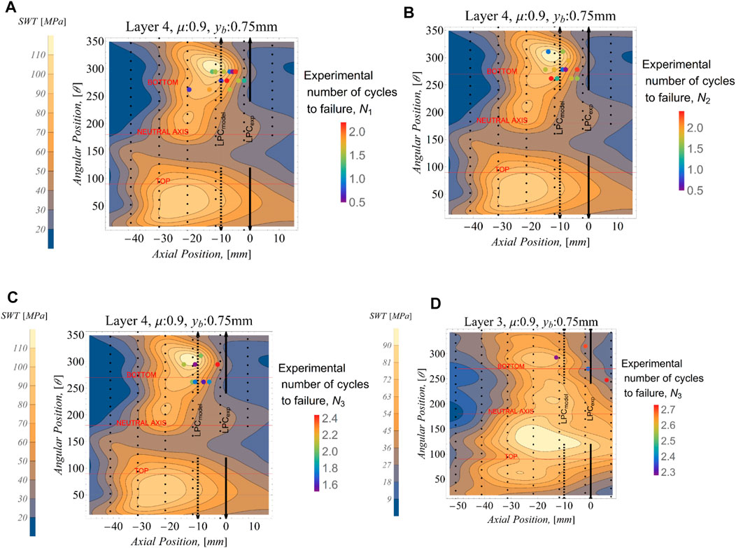
FIGURE 10. Location and number of cycles of Experimental Observation of Levesque Levesque (2005): (A) first wire failure, (B) second wire failure, (C) third wire failure on layer 4, and (D) third wire failure on layer 3; all for a bending amplitude of 0.75 mm. Indicated number of cycles are in millions (10⁶).

FIGURE 11

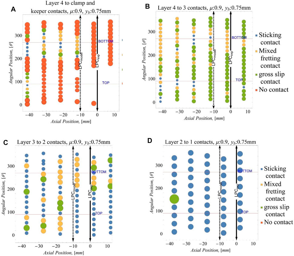
FIGURE 11. Indicator function G(E) for (A) layer 4 to clamp contacts, (B) layer 4 to layer 3 contacts, (C) layer 3 to layer 2 contacts, and (D) layer 2 to layer 1 contacts.

Furthermore, the LPC from the experiment of Levesque (2005) and that from the numerical model shown as a black double head arrow and a broken double head arrow in Figures 10, 11 show some difference. This difference in the location of the LPC between the model and experimental setup has been attributed by Lalonde et al. (2018) to plasticity effects that are not included in the numerical model. Indeed, it has been noted that the Timoshenko beam theory exhibits a stiffer response when in contact with a surface as compared with a full elasticity solution (Essenburg, 1975; Gasmi et al., 2012; Naghdi and Rubin, 1989). Nonetheless, the analysis provides estimates of the spatial variation of stresses that are sufficiently precise for the purpose of the fatigue analysis of multi-body systems such as conductors (Lalonde et al., 2018; Omrani et al., 2021).

Figure 12 shows the SWT distribution for other bending amplitudes. The $\stackrel{smoothened}{\overbrace{SW{T}_L|y_b\left(d,\theta \right)}}$ of Figure 12 and the wire fatigue resistance $f_{SW{T}_R}\left(SW{T}_R | N=N_i\right)$ are substituted in Equation 12 to obtain the probability of failure for each contact point. The results are shown as probability contour plots for the wires of layer 4 at bending amplitudes of 0.75, 0.6, 0.5, and 0.4 mm, respectively, in Figures 13, 14. For the case where the bending amplitude is 0.75 and 0.6 mm, the probabilities of failures are governed by the wires at the bottom in layer 4 for number of cycles ${10}^5 - {10}^6$. However, as the number of cycles increases to ${10}^7$, the probability of failure at the top of the conductor increases. In the case of lower bending amplitudes of 0.5 and 0.4 mm, the increment in size of the region of failure is less with the increasing number of cycles as compared to higher amplitudes. This shows that, for lower amplitudes, the number of wires at risk of failure is smaller.

FIGURE 12

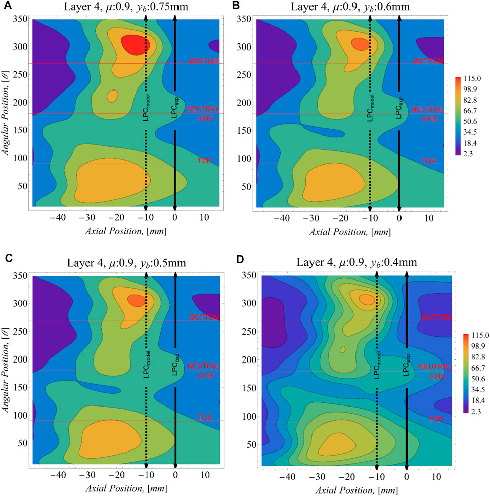
FIGURE 12. Maximum SWT distribution on the wires of layer 4 of the Bersfort conductor. (A) bending amplitude of 0.75 mm. (B) bending amplitude of 0.6 mm (C) bending amplitude of 0.5 mm (D) bending amplitude of 0.4 mm. Units of the SWT are in MPa.

FIGURE 13

FIGURE 13. Probability of failure for the wires in layer 4 of the Bersfort conductor at a bending amplitude of 0.75 mm (A–C) and 0.6 mm (D–F).

FIGURE 14

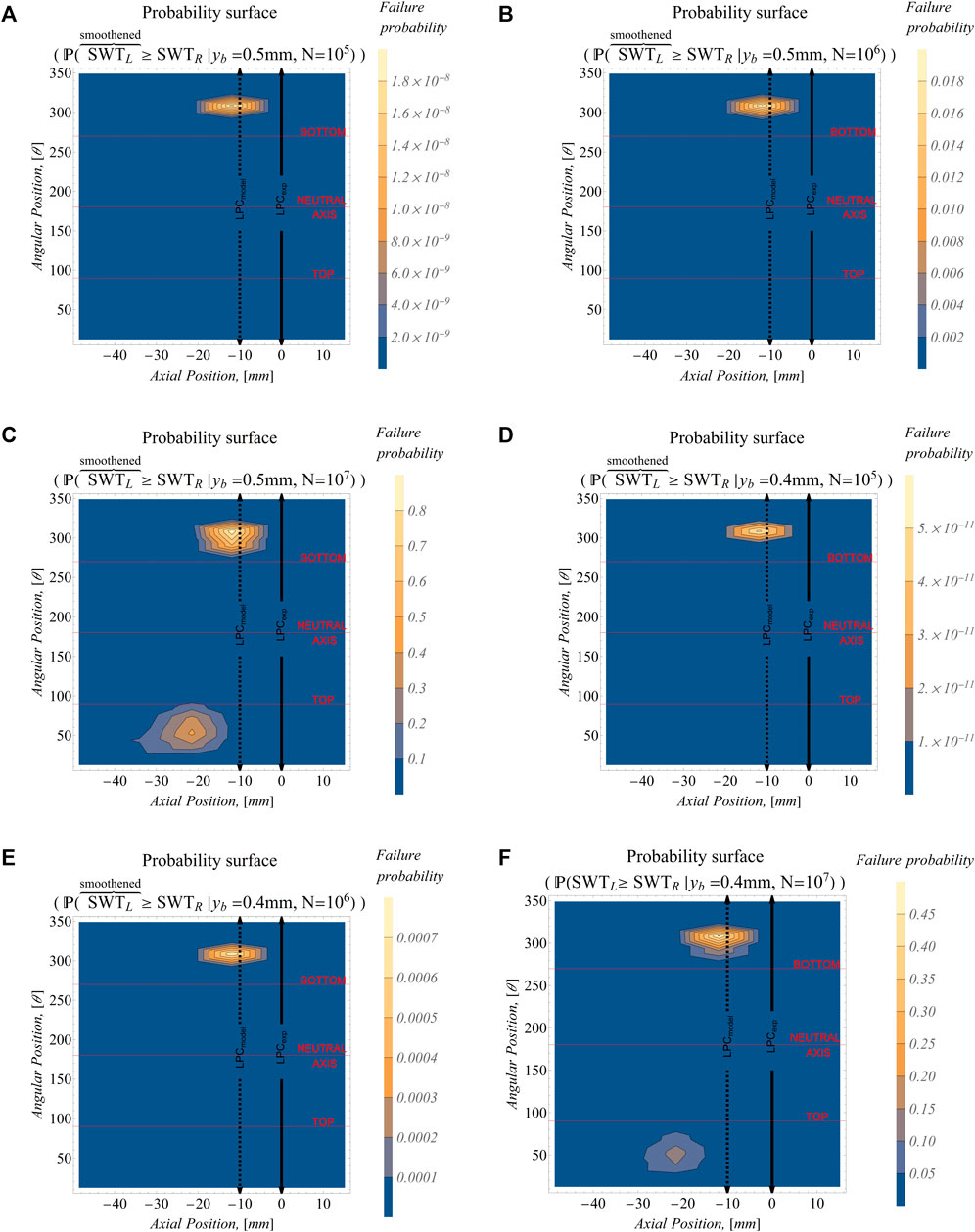
FIGURE 14. Probability of failure for the wires in layer 4 of the Bersfort conductor at a bending amplitude of 0.5 mm (A–C) and 0.4 mm (D–F).

Given the probabilities of failure for each contact point $\mathbb{P}\left(\stackrel{smoothened}{\overbrace{SW{T}_L | y_b\left(d,\theta \right)}}\ge \left(SW{T}_R|N=N_i\right)\right)$ and the fretting indicator function G(E), the probability of failure of the conductor can be obtained by using Equation 14. The results of these computations are fragility curves shown in terms of the cumulative distribution function (CDF) of $N |y_b$ in Figures 15, 16 for bending amplitudes 0.75, 0.6, 0.5 and 0.4 mm, respectively. The plots are shown for the first, second, and third wire failures.

FIGURE 15

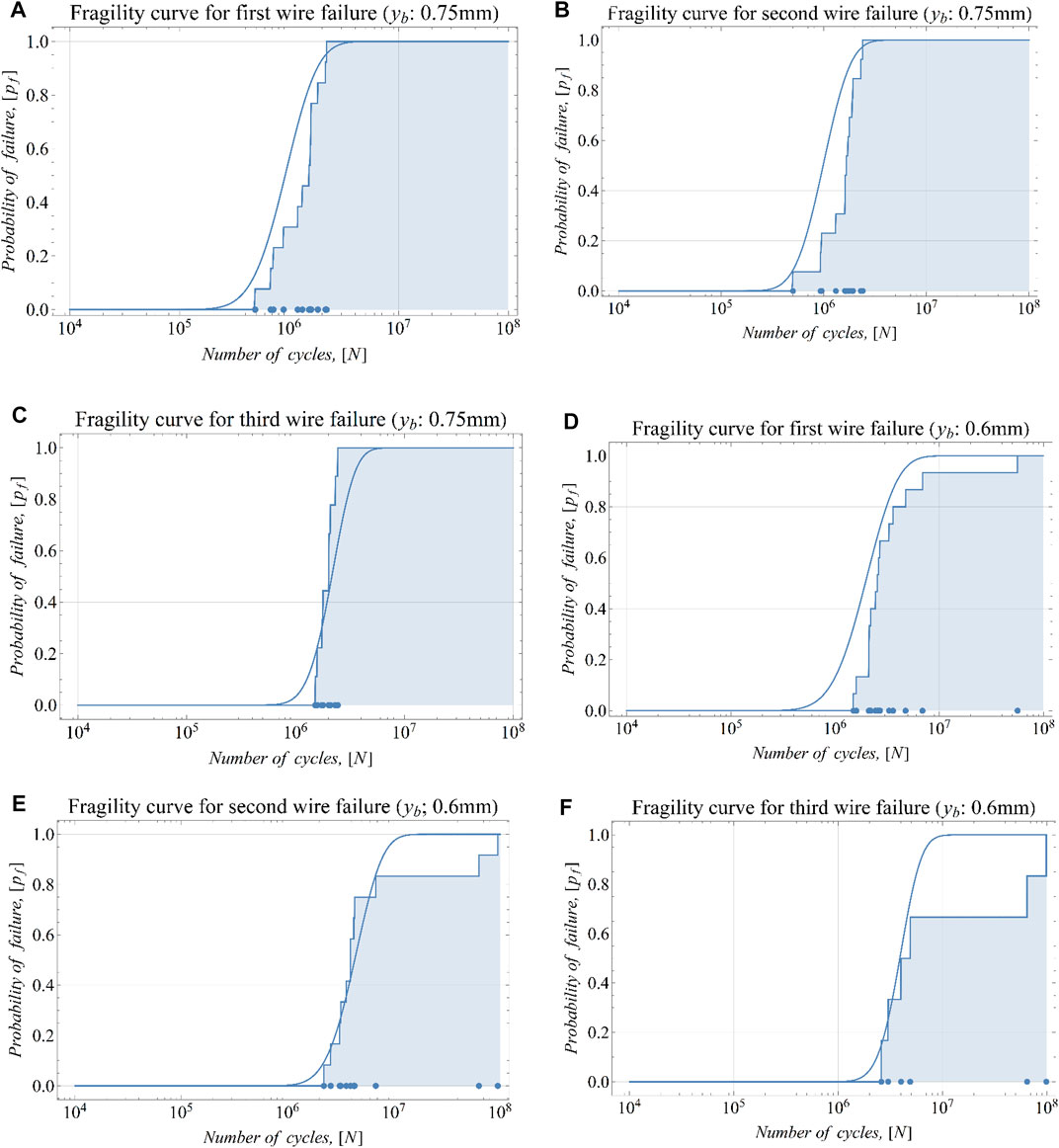
FIGURE 15. Fragility curves for the Bersfort conductor-clamp assembly. (A–C) Bending amplitude of 0.75 mm. (D–F) Bending amplitude of 0.6 mm.

FIGURE 16

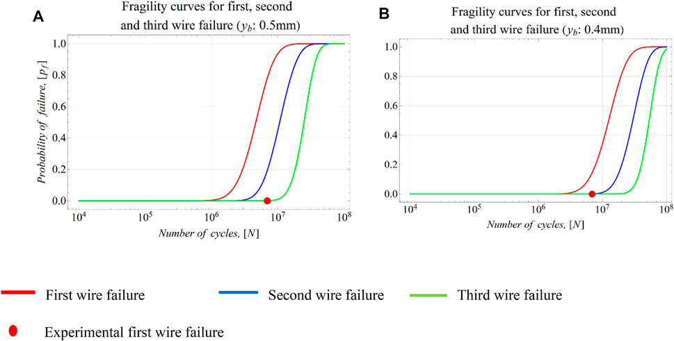
FIGURE 16. Fragility curves for the Bersfort conductor at a bending amplitude of (A) 0.5 mm and (B) 0.4 mm.

To validate the predicted fragility CDF, the empirical cumulative distribution functions (ECDF) for the experimental data in Levesque (2005) on the same Bersfort conductor are also presented. For the bending amplitudes 0.75 and 0.6 mm for which a reasonable amount of experimental data is available, the CDF compares well with the ECDF for the first, second, and third wire failures.

For a bending amplitude of 0.6 mm, the fragility curves given in Figures 15A–C show that there are outliers in the experimental data presented in Levesque (2005). The cause of these outliers is not known and may possibly be due to different experimental conditions.

Different models, exclusively derived from experimental data, such as the CIGRE Safe Border Line (CSBL) (CIGRE, 1979), the EPRI dataset (Cloutier et al., 2006), the safe limit of Hardy and Leblond (2001), and the confidence interval of Thomas et al. (2020), have been proposed for the fatigue resistance of overhead conductor-clamp systems for first wire failure. The stress–life predictions derived from the numerical model are compared to these empirical models in Figure 17. The SN curve for the numerical model is obtained by computing the quantile of the Poisson Binomial distribution for the first wire failure as:

$\mathbb{P}\left(N_p\le N|k\ge k\right)=p(18)$

where the values of the probability $p$ are {0.05, 0.5, 0.95}, which represents the fifth, 50th, and 95th fractiles of the SN curve and k = 1. SN curves for second and third wire failures can also be generated by using k = 2 and k = 3.

FIGURE 17

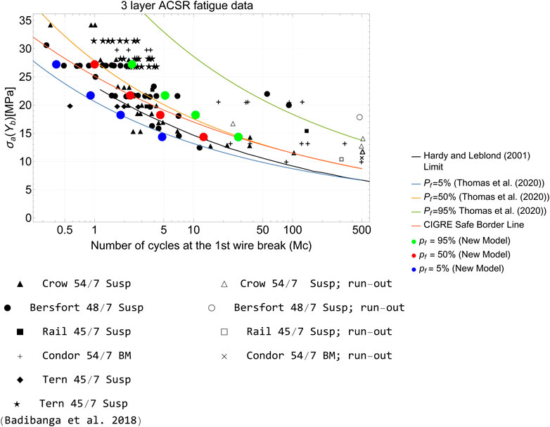
FIGURE 17. A comparison of the stress–life curves derived from the proposed framework for first wire failure with previous models. All black data points are from Cloutier et al. (2006) except otherwise stated.

For large amplitudes (0.75 mm), the median predicted life from the proposed model is close to the median curve proposed by Thomas et al. (2020). It is also noted that the CIGRE-CSBL is not a safe border line since it is above the 5% probability of failure predicted by the new model. Such a limitation of the CIGRE-CSBL has also been noted by Hardy and Leblond (2001). The results of the new model also show that the safe limit of Hardy and Leblond (2001) is also above the 5% probability of failure predicted by the new model and the model of Thomas et al. (2020).

It is also noted that the 95% confidence interval for the new model is narrower than the interval proposed in Thomas et al. (2020). This can be explained by the fact that conductor fatigue data in Cloutier et al. (2006) used by Thomas et al. (2020) include data using different experimental conditions and conductor-clamp types and configurations on the basis of idealized stress model.

In addition to the fragility curves and SN curves, the expected value and variance of the number of failed wires β as a function of number of cycles can be obtained (Wang, 1993):

$E\left(\mathcal{B}|N=N_i\right)=E\left({\displaystyle \sum _{m=1}^n{\mathbb{P}}_m\left(N=N_i\right)}\right)(19)$

$Var\left(\mathcal{B}|N=N_i\right)={\displaystyle \sum _{m=1}^n{\mathbb{P}}_m\left(N=N_i\right)\left(1-{\mathbb{P}}_m\left(N=N_i\right)\right)}(20)$

The conditional mean and variance of Eqs 19, 20 are compared to observed values in Table 3.

TABLE 3

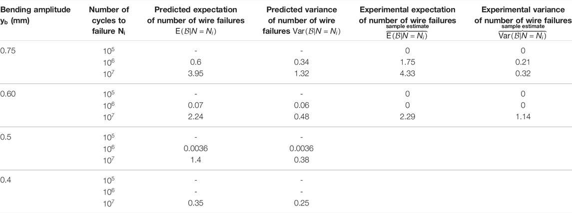
TABLE 3. Comparison of predicted number of wire failures against experimental observation.

The information in Table 3, can be used to supplement the fragility curves by considering both a target probability of failure for a conductor and an allowable number of wire failures for the conductor-clamp system. However, more data are needed to validate Equations 19, 20 for lower amplitudes.

Conclusion

A methodology for the derivation of fragility curves for electric overhead conductor-clamp systems has been presented. First, a finite element model of the conductor-clamp assembly is used to evaluate the contact stresses and fretting regime at all contact points between wires and between wires and clamp for a given amplitude of displacement. The state of stress at each contact is used to evaluate a fretting fatigue criterion based on the SWT and the potential for a mixed fretting fatigue regime that is most conducive to failure. For contacts that are characterized with a mixed fretting regime, the probability of failure as a function of number of cycles is evaluated as a function SWT by considering the distribution of SWT at failure as a function of number of cycles for fatigue data obtained from single aluminum wires. The probability of failure of the conductor as a function of number of cycles is then evaluated by considering a single, two, or three wires as the failure criterion. The model is validated by a comparison of the predicted location of failed wires as well as the number of cycles to failure with experimental data available in the literature. The presented methodology offers the following advantages and innovations:

• The conductor is not idealized as a single entity but models the conductor fatigue failure as a system of wires;

• The model accounts for the configuration of a conductor-clamp assembly, clamp radius, clamping torque, etc.;

• It provides predictions of single and multiple wire failures and avoids or reduces the number of tests that are performed in practice to derive SN curves for each type of conductor-clamp assembly;

• Fragility curves for a Bersfort conductor are presented for up to three wire failures for any amplitude of vibration;

• The SN model derived from the proposed method has much smaller variance than current models that combine experimental results from different conductor-clamp assemblies on the basis of the simple flexion model and significantly improves the accuracy of fatigue life predictions.

The next steps for future developments of the approach are to apply the procedure to the other conductor/clamp configurations, extend the analysis to damage accumulation rules that consider a combination of cycles of vibrations of different amplitude, and investigate procedures to extend the applicability of the model for conductor failures based on larger numbers of conductor wires. However, it is unlikely that the industry would adopt such a criterion considering the current practice in addition to the significant increase in the complexity of the analysis of stress redistribution that needs to be considered.

Data Availability Statement

The raw data supporting the conclusions of this article will be made available by the authors, without undue reservation.

Author Contributions

OT carried out the numerical modeling and probabilistic analysis, analyzed the result, and prepared the manuscript. LC supervised all phases of the research project, provided guidance on the probabilistic aspects of the project, and edited the manuscript. SL conceived the research project, supervised all phases of the research project, and edited the manuscript. All authors approved the submitted version of the article.

Funding

Funding for the research project was provided by the Natural Sciences and Engineering Research Council of Canada (NSERC), Funding program InnovÉÉ, FRQNT (through the strategic group CEISCE), Hydro-Québec, and Réseau de Transport d’Électricite (RTE).

Conflict of Interest

The authors declare that the research was conducted in the absence of any commercial or financial relationships that could be construed as a potential conflict of interest.

Publisher’s Note

All claims expressed in this article are solely those of the authors and do not necessarily represent those of their affiliated organizations, or those of the publisher, the editors, and the reviewers. Any product that may be evaluated in this article, or claim that may be made by its manufacturer, is not guaranteed or endorsed by the publisher.

References

Babuška, I., Sawlan, Z., Scavino, M., Szabó, B., and Tempone, R. (2016). Bayesian Inference and Model Comparison for Metallic Fatigue Data. Comput. Methods Appl. Mech. Eng. 304, 171–196. doi:10.1016/j.cma.2016.02.013

CrossRef Full Text | Google Scholar

Badibanga, R., Miranda, T., Rocha, P., Ferreira, J., da Silva, C., and Araújo, J. (2018). The Effect of Mean Stress on the Fatigue Behaviour of Overhead Conductor Function of the H/w Parameter. MATEC Web Conf. 165, 11001. doi:10.1051/matecconf/201816511001

CrossRef Full Text | Google Scholar

Baumann, R., and Novak, P. (2017). Efficient Computation and Experimental Validation of ACSR Overhead Line Conductors under Tension and Bending. CIGRE Sci. Eng. 9, 5–16.

Google Scholar

Cardou, A., Cloutier, L., Lanteigne, J., and M'Boup, P. (1990). Fatigue Strength Characterization of ACSR Electrical Conductors at Suspension Clamps. Electric Power Syst. Res. 19, 61–71. doi:10.1016/0378-7796(90)90008-q

CrossRef Full Text | Google Scholar

CIGRE (1979). Recommendation for the Evaluation of the Lifetime of Transmission Line Conductors (Electra N 63).

Google Scholar

CIGRE-WG-B2.30 (2010). Engineering Guidelines Relating to Fatigue Endurance Capability of Conductor/Clamp Systems.

Google Scholar

Cloutier, L., Goudrea, S., and Cardou, A. (2006). “Fatigue of Overhead Conductors,” in EPRI Transmission Line Reference Book: Wind-Induced Conductor Motion. Editors J. K. Chan, D. G. Havard, C. B. Rawlins, and J. Weisel. 2nd ed. (Palo Alto, CA: EPRI).

Google Scholar

Cloutier, L., and Leblond, A. (2007). Fatigue Endurance Capability of Conductor/Clamp Systems (Update of Present Knowledge). CIGRE.

Google Scholar

Degat, P. R., Zhou, Z. R., and Vincent, L. (1997). Fretting Cracking Behaviour on Pre-stressed Aluminium alloy Specimens. Tribology Int. 30 (3), 215–223. doi:10.1016/S0301-679X(96)00046-1

CrossRef Full Text | Google Scholar

Essenburg, F. (1975). On the Significance of the Inclusion of the Effect of Transverse Normal Strain in Problems Involving Beams with Surface Constraints. J. Appl. Mech. 42 (1), 127–132. doi:10.1115/1.3423502

CrossRef Full Text | Google Scholar

Gasmi, A., Joseph, P. F., Rhyne, T. B., and Cron, S. M. (2012). The Effect of Transverse normal Strain in Contact of an Orthotropic Beam Pressed against a Circular Surface. Int. J. Sol. Structures 49 (18), 2604–2616. doi:10.1016/j.ijsolstr.2012.05.022

CrossRef Full Text | Google Scholar

Goudreau, S., Levesque, F., Cardou, A., and Cloutier, L. (2010). Strain Measurements on ACSR Conductors during Fatigue Tests III-Strains Related to Support Geometry. IEEE Trans. Power Deliv. 25 (4), 3007–3016. doi:10.1109/TPWRD.2010.2045399

CrossRef Full Text | Google Scholar

Hardy, C., and Leblond, A. (2001). “Statistical Analysis of Stranded Conductor Fatigue Endurance Data,” in Proceeding of the Fouth International Symposium on Cable Dynamics, Montreal, Canada.

Google Scholar

Hathout, I. (2016). “Fuzzy Probabilistic Expert System for Overhead Conductor Assessment and Replacement,” Fuzzy Probabilistic Expert System for Overhead Conductor Assessment and Replacement, San Diego, United States.

Google Scholar

Hills, D. A., and Nowell, D. (1994). Mechanics of Fretting Fatigue Springer-Science. Berlin, Germany: Springer.

Google Scholar

Jang, Y. H., and Barber, J. R. (2011). Effect of Phase on the Frictional Dissipation in Systems Subjected to Harmonically Varying Loads. Eur. J. Mech. - A/Solids 30 (3), 269–274. doi:10.1016/j.euromechsol.2011.01.008

CrossRef Full Text | Google Scholar

Kaufman, J. G. (2008). Properties of Aluminum Alloys: Fatigue Data and Effects of Temperature, Product Form, and Processing. Ohio, USA: ASM International.

Google Scholar

Lalonde, S., Guilbault, R., and Langlois, S. (2017). Modeling Multilayered Wire Strands, a Strategy Based on 3D Finite Element Beam-To-Beam Contacts - Part II: Application to Wind-Induced Vibration and Fatigue Analysis of Overhead Conductors. Int. J. Mech. Sci. 126, 297–307. doi:10.1016/j.ijmecsci.2016.12.015

CrossRef Full Text | Google Scholar

Lalonde, S., Guilbault, R., and Langlois, S. (2018). Numerical Analysis of ACSR Conductor-Clamp Systems Undergoing Wind-Induced Cyclic Loads. IEEE Trans. Power Deliv. 33 (4), 1518–1526. doi:10.1109/TPWRD.2017.2704934

CrossRef Full Text | Google Scholar

Levesque, F. (2005). “Etude de l'applicabilite de la regle de Palmgren-Miner aux conducteurs electriques sous chargements de flexion cyclique par blocs,”. MSc (Quebec City, Canada: Universite Laval).

Google Scholar

Naghdi, P. M., and Rubin, M. B. (1989). On the Significance of normal Cross-Sectional Extension in Beam Theory with Application to Contact Problems. Int. J. Sol. Structures 25 (3), 249–265. doi:10.1016/0020-7683(89)90047-4

CrossRef Full Text | Google Scholar

Omrani, A., Langlois, S., Van Dyke, P., Lalonde, S., Karganroudi, S. S., and Dieng, L. (2021). Fretting Fatigue Life Assessment of Overhead Conductors Using a Clamp/conductor Numerical Model and Biaxial Fretting Fatigue Tests on Individual Wires. Fatigue Fract Eng. Mat Struct. 44 (6), 1498–1514. doi:10.1111/ffe.13444

CrossRef Full Text | Google Scholar

Pascual, F. G., and Meeker, W. Q. (1997). Analysis of Fatigue Data with Runouts Based on a Model with Nonconstant Standard Deviation and a Fatigue Limit Parameter. J. Test. Eval. 25 (3), 292–301. doi:10.1520/JTE11341J

CrossRef Full Text | Google Scholar

Poffenberger, J. C., and Swart, R. L. (1965). Differential Displacement and Dynamic Conductor Strain. IEEE Trans. Power Appar. Syst. 84 (4), 281–289. doi:10.1109/TPAS.1965.4766192

CrossRef Full Text | Google Scholar

Pouliot, N., Rousseau, G., Gagnon, D., Valiquette, D., Leblond, A., Montambault, S., et al. (2020). “An Integrated Asset Management Strategy for Trasmission Line Conductors, Based on Robotics, Sensors, and Aging Modelling,” in Paper presented at the Engineering Assets and Public Infrastructures in the Age of Digitalization Confrence, Norway.

Google Scholar

Rawlins, C. B. (1979). “Fatigue of Overhead Conductors,” in EPRI Transmission Line Reference Book: Wind-Induced Conductor Motion (Palo Alto, CA: EPRI).

Google Scholar

Redford, J. A., Gueguin, M., Nguyen, M. C., Lieurade, H.-P., Yang, C., Hafid, F., et al. (2019). Calibration of a Numerical Prediction Methodology for Fretting-Fatigue Crack Initiation in Overhead Power Lines. Int. J. Fatigue 124, 400–410. doi:10.1016/j.ijfatigue.2019.03.009

CrossRef Full Text | Google Scholar

Rocha, P. H. C., Díaz, J. I. M., Silva, C. R. M., Araújo, J. A., and Castro, F. C. (2019). Fatigue of Two Contacting Wires of the ACSR Ibis 397.5 MCM Conductor: Experiments and Life Prediction. Int. J. Fatigue 127, 25–35. doi:10.1016/j.ijfatigue.2019.05.033

CrossRef Full Text | Google Scholar

Said, J., Garcin, S., Fouvry, S., Cailletaud, G., Yang, C., and Hafid, F. (2020). A Multi-Scale Strategy to Predict Fretting-Fatigue Endurance of Overhead Conductors. Tribology Int. 143, 106053. doi:10.1016/j.triboint.2019.106053

CrossRef Full Text | Google Scholar

Thomas, O. O., Chouinard, L., and Langlois, S. (2020). “A Probabilistic Stress-Life Model for Fretting Fatigue of Aluminum Conductor Steel Reinforced Cable-Clamp Systems,” in Engineering Assets and Public Infrastructures in the Age of Digitalization. Lecture Notes in Mechanical Engineering (Berlin, Germany: Springer).

CrossRef Full Text | Google Scholar

Wang, Y. H. (1993). On the Number of Successes in Independent Trials. Stat. Sinica 3, 295–312.

Google Scholar

Zhou, Z. R., Cardou, A., Goudreau, S., and Fiset, M. (1994). Fretting Patterns in a Conductor?clamp Contact Zone. Fat Frac Eng. Mat Struct. 17 (6), 661–669. doi:10.1111/j.1460-2695.1994.tb00264.x

CrossRef Full Text | Google Scholar

Zhou, Z. R., and Vincent, L. (1995). Mixed Fretting Regime. Wear 181-183, 531–536. doi:10.1016/0043-1648(95)90168-X

CrossRef Full Text | Google Scholar

Nomenclature

$Y_b$ bending amplitude at 89 mm from the last point of contact

${\sigma }_a$ / ${\epsilon }_a$ idealized stress resulting from bending amplitude

$F_c$ clamping force

T conductor tension

$T_0$ initial tension

β number of failed wires

β bending angle

${\beta }_p$ bending angle at passive end of conductor

${\beta }_0$ bending angle at the active end of conductor

EI bending stiffness of conductor

$E_a$ elastic modulus of aluminum wire

$E_i$ elastic modulus of wire i

E energy dissipated at a contact

$I_i$ moment of inertia of wire i

$d_c$ diameter of conductor

$d_i$ diameter of wire i

$d$ gap function between slave and master element

$d_j$ axial position of wire center line j

$\theta$ angular position of wire center line

N number of cycles

SN stress-number of cycles

v poisson ratio

$n_i$ number of wires in layer i

$r_c$ radius of slave beam element

$r_t$ radius of master beam element

$\mathrm{\Delta }\sigma$ stress range

$Q\left(t\right)$ tangential force of slave node at time t

u(t) sliding distance of slave node at time t

SWT Smith-Watson-Topper fatigue criteria

$SW{T}_L | Y_b=y$ SWT value obtained from finite element model at a given bending amplitude

$SW{T}_R | N=N_i$ SWT value obtained from plain fatigue model of aluminum wires at a given number of cycles

$f\left(SW{T}_R | N=N_i\right)$ probability density function of plain fatigue model of aluminum wires

$\mu \left(SW{T}_R\right)$ mean of the distribution of plain fatigue model of aluminum wires

$\sigma \left(SW{T}_R\right)$ standard deviation of plain fatigue model of aluminum wires

$SW{T}_{L_m} | y_b$ SWT of wire segment m

${\sigma }_1$ maximum principal stress

$G\left(E\right)$ indicator function for fretting regimes

$G\left(E_{m,\mathrm{ℱ}}\right)$ indicator function for fretting regimes for wire segment m with contact at the top and bottom

ℙ(X) probability of occurrence of event X

$\mathcal{E}\left(X\right)$ expectation of a random variable X

$\mathbb{V}\mathbb{A}\mathbb{R}\left(\mathit{X}\right)$ variance of a random variable X

k number of wire failures

$k\left({\sigma }_d, {\sigma }_{\theta }\right)$ two-dimension gaussian kernel with parameters ${\sigma }_d, {\sigma }_{\theta }$

$\stackrel{smoothened}{\overbrace{SW{T}_L|y_b\left(d_j,{\theta }_j\right)}}$ SWT value for a given bending amplitude at wire axial and angular position obtained from finite element model and averaged with Gaussian kernel $k\left({\sigma }_d, {\sigma }_{\theta }\right)$

LPC last point of contact between conductor and clamp

$LP{C}_{model}$ last point of contact observed in finite element model

$LP{C}_{exp}$ last point of contact observed in experiment

KE keeper edge

PDF probability density function

EPDF empirical probability density function

CDF cumulative distribution function

ECDF empirical cumulative distribution function

MPC multiple point constraint

CONTA177 slave contact element on beam or shell elements

TARGE170 master contact element on beam or shell elements