Tension Estimation Method for Cable With Damper Using Natural Frequencies With Uncertain Modal Order

In the maintenance of cable structures, such as cable-stayed bridges, it is necessary to estimate the tension acting on the cables. In current Japanese practice, the cable tension is estimated from the cable’s natural frequency using vibration-based methods. However, in recent years, dampers have been installed onto the cables to suppress aerodynamic vibrations. Because the damper changes the cable’s natural frequencies, the methods used for cables without dampers are not appropriate for cables with dampers. With this background, the authors previously proposed a method (Method 0F) for estimating the tension of a cable with a damper from the natural frequencies and their modal order. Method 0F partially ignores the imaginary part of the complex natural frequencies to simplify the problem. This study proposes a new method (Method 1F) that does not ignore the imaginary part of a complex natural frequency. Method 1F still needs both the natural frequencies and their modal order to be input. If the modal order is not correctly specified, the accuracy deteriorates. Therefore, a new method (Method 2F) that only requires the natural frequencies is also proposed. The validity of the proposed methods was confirmed by numerical simulations and experiments. The numerical and experimental verifications confirmed that the new methods were superior compared with previous methods, and that Method 2F has the highest effectiveness.

1 Introduction

In the maintenance of cable structures, such as cable-stayed bridges and extra-dosed bridges, the estimation of the tension acting on the cables plays an important role. The tension of cables is measured using a direct measurement method with a load cell, or an indirect estimation method that considers the cable’s vibration characteristics. The former method is difficult to use in practical situations owing to the high cost and installation of complicated devices. Therefore, the latter method is used in practice because it is easy to implement and achieves a high estimation accuracy.

In current Japanese practice, the tension of cables is mainly estimated using the vibration method proposed by Shinke et al. (1980) or the higher-order vibration method proposed by Yamagiwa et al. (2000), which considers the cable’s natural frequencies.

The vibration method (Shinke et al., 1980; Zui et al., 1996) is based on the theory of strings, whereby the cable’s tension is proportional to the square of the frequency. However, the actual cable is not a pure thread, and the effect of the bending stiffness is not negligible. Therefore, the effect of the bending stiffness is considered in the form of a correlation factor. In this method, it is necessary to determine the bending stiffness of the cable in advance. However, the correct bending stiffness is difficult to determine because bridge cables are typically prestressed steel strands rather than single-steel wires.

To address this problem, Yamagiwa et al. (2000) proposed a higher-order vibration method based on the tensioned Bernoulli–Euler beam theory. In this method, the natural frequency of the i^th mode is expressed by a polynomial of modal order i with the bending stiffness and tension as coefficients. The tension and bending stiffness of the cable are simultaneously estimated using the natural frequencies of multiple modes. The bending stiffness does not need to be determined in advance. Currently, this method is more frequently used to estimate tension.

In addition to the above-mentioned studies, various studies based on modal data have investigated cable tension estimation techniques. For example, studies have employed methods using the mode shapes in addition to the natural frequencies (Chen et al., 2016; Chen et al., 2018; Yan et al., 2019), methods dealing with complicated boundary conditions (Chen et al., 2016; Chen et al., 2018; Yan et al., 2019), a method dealing with the uncertain boundary condition of a short cable by introducing an additional mass block (Li et al., 2021), methods dealing with inclined cables (Kim and Park, 2007; Ma, 2017), a method dealing with a cable with flexible supports (Foti et al., 2020), a method dealing with environmental temperature variation (Ma et al., 2021), methods for two cables connected by an intersection clamp (Furukawa et al., 2022), a method using power spectrum and cepstrum (Feng, et al., 2010), a method using a finite element method (Gan et al., 2019), a method using a genetic algorithm and particle swarm optimization (Zarbaf et al., 2017), and a method using neural networks (Zarbaf et al., 2018).

In recent years, the length of bridges and the length of installed cables have been increasing. Because the damping performance of the cable itself is small, the vibration caused by the wind is notable. To suppress the aerodynamic vibration of the cables, dampers are installed onto the cables. In the maintenance of cables with dampers, the direct use of the vibration method or the higher-order vibration method is inappropriate because the damper changes the natural frequencies. Typically, the damper increases the cable’s natural frequencies. Because a cable with a large tension has high natural frequencies, the tension will be overestimated if the vibration method or the higher-order vibration method is directly applied to a cable with a damper. Therefore, in practice, the damper is detached from the cable before the natural frequencies of the cable without a damper are measured, and the damper is then reattached to the cable. Because the process of detaching and attaching the damper is time-consuming and labor-intensive, it is useful to develop a tension estimation method for a cable with a damper to estimate the cable tension without detaching the damper from the cable.

Previous studies on cables with dampers have mostly focused on the optimal design of dampers for suppressing the cable amplitude (Pacheco et al., 1993; Tabatabai and Mehrabi, 2000; Izzi et al., 2016; Lazar et al., 2016; Shi and Zhu, 2018; Javanbakht et al., 2019; Krenk, 2000, and have not dealt with the tension estimation method. Krenk (2000) derived a theoretical equation to obtain complex eigenfrequencies, from which the natural frequencies and damping ratios were subsequently obtained. However, the cable was modeled as a string, and the effect of the cable’s bending stiffness was ignored. Therefore, these equations cannot be used to estimate the tension of a cable with bending stiffness.

Studies dealing with the tension estimation method for a cable with a damper are still scarce. Yang et al. (2020) proposed a tension estimation method for cables with two intermediate supports (dampers). They assumed a damper whose reaction force is the product of the damper’s spring constant and displacement. The damping force that decays the displacement is ignored. Moreover, the damper’s spring constant is assumed to be known. However, because the damper’s performance gradually degrades because of aging, it is occasionally difficult to obtain the spring constant of an actual damper.

Shan et al. (2019) estimated the tension of a cable with a supplemental damper. A viscous shear damper with a spring constant and a damping coefficient is assumed. This method assumes that the cable’s bending stiffness and damper’s damping coefficient are known, and adopts a two-step identification. In the first step, the damper’s spring constant is identified. In the second step, the cable’s tension is identified using the damper’s spring constant. However, as stated above, it is not always possible to accurately obtain the cable’s bending stiffness and damper’s damping coefficient.

Hou et al. (2020) proposed a cable tension estimation method by adding virtual supports using the substructure isolation method. Their method virtually separates a cable section from the overall structure by adding virtual supports and avoids unknown factors such as the boundary conditions and cable length. It is considered that their method can be applied to a cable with a damper by separating the cable section without a damper. However, this method requires virtual supports, and the installation and removal of virtual supports is time-consuming and laborious compared with the high-order vibration method without additional members.

The authors have been involved in research to develop a new tension estimation method for a cable with a damper. Using the concept of the higher-order vibration method (Yamagiwa et al., 2000), a theoretical equation for estimating the natural frequencies of a cable with a damper has been derived (Furukawa et al., 2021a). In the authors’ previous method, the theoretical equation for estimating the complex natural frequencies from the tension and bending stiffness of the cable and the damper parameters was derived. The natural frequencies observed by a field experiment correspond to the real part of the complex natural frequencies. Therefore, by inversely solving the theoretical equation, the tension and bending stiffness of the cable and the damper parameters can be estimated from the natural frequencies. The cable’s bending stiffness and the damper parameters do not need to be determined in advance and can instead be estimated simultaneously with the cable tension.

The authors’ previous method can estimate the cable tension with good accuracy (Furukawa et al., 2021a), but requires improvement with regard to two points.

First, the previously proposed method partially ignores the imaginary part of the complex natural frequency to simplify the inverse problem. However, the tension estimation accuracy may deteriorate when the imaginary part of the complex natural frequency is large. Therefore, accuracy improvement can be expected if the first point is addressed, particularly when the imaginary part of the complex natural frequency is large.

The second point is that the previously proposed method requires the natural frequencies and their modal order as a set. If the modal order is erroneously assigned, the tension estimation accuracy deteriorates. Moreover, the modal order has to be correctly assigned to each natural frequency, which is occasionally difficult.

With this background, this study proposes new tension estimation methods to improve the above-mentioned points. In Section 2, the previously proposed method (Method 0F) for estimating the tension of a cable with a damper is first described. Next, the improvements in the two above-mentioned points are explained. Section 3 presents two new methods (Methods 1F and 2F). Method 1F improves the first point, while Method 2F improves both points. Section 4 presents the numerical verification of 90 numerical models. The natural frequencies of a cable with a damper were calculated for 90 models and input into the proposed methods. The estimated tension is compared with the assumed true value, and the accuracy and validity of the proposed methods are discussed. Section 5 presents the experimental verification of the proposed methods. The estimated tension is compared with the tension measured by the load cell, and the accuracy and validity of the proposed methods are discussed.

2 Previously Proposed Method for Cable Tension Estimation (Method 0F)

2.1 Vibration Equation of Tensioned Bernoulli-Euler Beam

In the methods proposed by the authors, the cable is considered a tensioned Bernoulli–Euler beam and its vibration equation is explained in this section.

The vibration equation for a tensioned Bernoulli–Euler beam can be written as the following partial differential equation:

$\rho A\frac{{\partial }^{2}y\left(x,t\right)}{\partial t^2}+EI\frac{{\partial }^{4}y\left(x,t\right)}{\partial x^4}-T\frac{{\partial }^{2}y\left(x,t\right)}{\partial x^2}=0(1)$

where $y\left(x,t\right)$ is the deflection, which is a function of position $x$ and time $t$; $\rho$ is the density; $A$ is the cross-sectional area; $EI$ is the bending stiffness; and $T$ is the tension.

The partial differential equation can be solved using the variable separation method. The deflection $y\left(x,t\right)$ is transformed as follows:

$y\left(x,t\right)=Y\left(x\right)\text{exp}\left(j\omega t\right)(2)$

where $Y\left(x\right)$ is the modal function of position $x$, $j$ is an imaginary unit, and $\omega$ is the circular frequency.

By substituting Eq. 2 into Eq. 1, the following ordinary differential equation for function $Y\left(x\right)$ can be derived:

$-\rho A{\omega }^{2}Y\left(x\right)+EI\frac{d^{4}Y\left(x\right)}{d{x}^4}-T\frac{d^{2}Y\left(x\right)}{d{x}^2}=0(3)$

The general solution of Eq. 3 is obtained as follows:

$Y\left(x\right)=C_1\text{cos}\alpha x+C_2\text{sin}\alpha x+C_3\text{cosh}\beta x+C_4\text{sinh}\beta x(4)$

where $C_1$, $C_2$, $C_3$, and $C_4$ are the integration constants; $\alpha$ and $\beta$ are expressed, respectively, as follows:

$\alpha =\sqrt{\sqrt{{\left(\frac{T}{2EI}\right)}^2+\frac{\rho A{\omega }^2}{EI}}-\frac{T}{2EI}}(5)$

$\beta =\sqrt{\sqrt{{\left(\frac{T}{2EI}\right)}^2+\frac{\rho A{\omega }^2}{EI}}+\frac{T}{2EI}}(6)$

2.2 Authors’ Previously Proposed Method (Method 0F)

2.2.1 Theoretical Equation for Estimating Natural Frequencies

This section explains the previously proposed method for estimating the tension of a cable with a damper from the natural frequencies (Method 0F). Figure 1 shows the analytical model of a cable with a damper and simple supports at the two ends. The damper shown in Figure 1 is a viscous shear damper with a spring constant $k$ and damping constant $c$. The cable length is $L$, and the distance from the damper position to the left and right ends is $L_1$ and $L_2\left(=L-L_1\right)$, respectively. The deflection of the cable on the left and right sides with regard to the damper position $x$ is denoted as $y_1\left(x,t\right)$ and $y_2\left(x,t\right)$, respectively. The deflection is expressed similarly to Eq. 2, as follows:

$y_1\left(x,t\right)=Y_1\left(x\right)\text{exp}\left(j\omega t\right)(7)$

$y_2\left(x,t\right)=Y_2\left(x\right)\text{exp}\left(j\omega t\right)(8)$

where $Y_1\left(x\right)$ and $Y_2\left(x\right)$ are the modal functions on the left and right sides of the cable, respectively, with regard to the damper position. The general solutions of $Y_1\left(x\right)$ and $Y_2\left(x\right)$ are expressed as follows:

$Y_1\left(x\right)=D_1\text{cos}\alpha x+D_2\text{sin}\alpha x+D_3\text{cosh}\beta x+D_4\text{sinh}\beta x\left(0\le x\le L_1\right)(9)$

$Y_2\left(x\right)=D_5\text{cos}\alpha \left(x-L_1\right)+D_6\text{sin}\alpha \left(x-L_1\right)+D_7\text{cosh}\beta \left(x-L_1\right)+D_8\text{sinh}\beta \left(x-L_1\right)\left(L_1\le x\le L\right)(10)$

where $D_1$, $D_2$, $D_3$, $D_4$, $D_5$, $D_6$, $D_7$, and $D_8$ are the integration constants, and $\alpha$ and $\beta$ are expressed by Eqs. 5, 6, respectively.

FIGURE 1

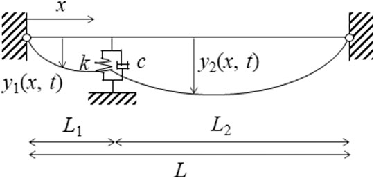
FIGURE 1. A model for a cable with a damper.

Because there are eight integration constants, eight boundary conditions are necessary. Four boundary conditions are established at the two ends ($x=0$ and $x=L$), that is, the deflection is zero and the second derivative of deflection is also zero owing to the simple supports (Y₁(0) = 0, d²Y₁(0)/dx² = 0, Y2(L) = 0, d²Y₂(L)/dx² 0). Three boundary conditions are established at the damper position ($x=L_1$), that is, the deflection, the deflection angle, and the second derivative of deflection are continuous ($Y_1\left(L_1\right)=Y_2\left(L_1\right)$, $d{Y}_1\left(L_1\right)/dx=d{Y}_2\left(L_1\right)/dx$, $d^2{Y}_1\left(L_1\right)/d{x}^2=d^2{Y}_2\left(L_1\right)/d{x}^2$). Moreover, the force exerted on the cable by the damper is equal to the shear force change of the cable at the damper position ($EI{d}^3{Y}_1\left(L_1\right)/d{x}^3-EI{d}^3{Y}_2\left(L_1\right)/d{x}^3=k{Y}_1\left(L_1\right)+j\omega c{Y}_1\left(L_1\right)$).

By substituting Eqs. 9, 10 into the eight boundary conditions, the following equation is obtained:

$\text{sin}\alpha L\left\{{\alpha }^2+{\beta }^2+\frac{k^{\ast }}{EI}\left(\frac{\text{sin}\alpha L_1\text{cos}\alpha L_1}{\alpha }-\frac{\text{sinh}\beta L_1\text{sinh}\beta L_2}{\beta \text{sinh}\beta L}\right)\right\}-\text{cos}\alpha L\left(\frac{k^{\ast }}{EI}\frac{{\text{sin}}^2\alpha L_1}{\alpha }\right)=0(11)$

where $k^{\ast }$ is the complex stiffness of the damper. The unified notation $k^{\ast }$ is used to model various types of dampers, as follows:

$k^{\ast }=\{\begin{array}{cc}{k}_u+j{k}_v& \left(\text{high}-\text{damping}\text{rubber}\text{damper}\right)\\ k+j\omega c& \left(\text{viscous}\text{shear}\text{damper}\right)\end{array}(12)$

In the case of the high-damping rubber damper, the complex stiffness $k^{\ast }$ is expressed with $k_u$ and $k_v$, which are the real and imaginary parts of the complex stiffness, respectively. In the case of the viscous shear damper, the complex stiffness $k^{\ast }$ is expressed with a spring constant $k$ and damping coefficient $c$.

Then, Eq. 11 can be transformed as follows:

$\text{sin}\left(\alpha L-\theta \right)=0(13)$

where

$\text{tan}\theta =\frac{\frac{k^{\ast }}{EI}\frac{{\text{sin}}^2\alpha L_1}{\alpha }}{{\alpha }^2+{\beta }^2+\frac{k^{\ast }}{EI}\left(\frac{\text{sin}\alpha L_1\text{cos}\alpha L_1}{\alpha }-\frac{\text{sinh}\beta L_1\text{sinh}\beta L_2}{\beta \text{sinh}\beta L}\right)}(14)$

Eq. 13 has infinite solutions for $\alpha$. These solutions are expressed with a positive integer $i$.

$\begin{array}{cc}{\alpha }_{i}L-{\theta }_i=i\pi & i=\mathrm{1,2},\dots .\end{array}(15)$

By substituting Eq. 5 into Eq. 15, the natural circular frequency ${\omega }_i$ of the $i$^th mode can be obtained as follows:

$\begin{array}{cc}{\omega }_i^2=\frac{{\pi }^{4}EI}{\rho A{L}^4}{\left(i+\frac{{\theta }_i}{\pi }\right)}^4+\frac{{\pi }^{2}T}{\rho A{L}^2}{\left(i+\frac{{\theta }_i}{\pi }\right)}^2& i=\mathrm{1,2},\dots \end{array}(16)$

Finally, the theoretical equation for estimating the natural frequencies $f_i^t$ of the $i$^th mode, and the relevant equations, are expressed as follows:

$f_i^t=\sqrt{\frac{{\pi }^{2}EI}{4\rho A{L}^4}{\left(i+\frac{{\theta }_i}{\pi }\right)}^4+\frac{T}{4\rho A{L}^2}{\left(i+\frac{{\theta }_i}{\pi }\right)}^2}i=\mathrm{1,2},\dots (17)$

${\theta }_i={\text{tan}}^{-1}\frac{\frac{k_i^{\ast }}{EI}\frac{{\text{sin}}^2{\alpha }_i{L}_1}{{\alpha }_i}}{{\alpha }_i^2+{\beta }_i^2+\frac{k_i^{\ast }}{EI}\left(\frac{\text{sin}{\alpha }_i{L}_1\text{cos}{\alpha }_i{L}_1}{{\alpha }_i}-\frac{\text{sinh}{\beta }_i{L}_1\text{sinh}{\beta }_i{L}_2}{{\beta }_i\text{sinh}{\beta }_{i}L}\right)}(18)$

${\alpha }_i=\sqrt{\sqrt{{\left(\frac{T}{2EI}\right)}^2+\frac{\rho A{\left(2\pi f_i^t\right)}^2}{EI}}-\frac{T}{2EI}}(19)$

${\beta }_i=\sqrt{\sqrt{{\left(\frac{T}{2EI}\right)}^2+\frac{\rho A{\left(2\pi f_i^t\right)}^2}{EI}}+\frac{T}{2EI}}(20)$

$k_i^{\ast }=\{\begin{array}{cc}{k}_u+j{k}_v& \left(\text{high}-\text{damping}\text{rubber}\text{damper}\right)\\ k+j\left(2\pi f_i^t\right)c& \left(\text{viscous}\text{shear}\text{damper}\right)\end{array}(21)$

From the cable parameters, namely, $\rho$, $A$, $L$, $EI$, and $T$, and the damper parameters $k_u$ and $k_v$ or $k$ and $c$, the $i$^th mode natural frequencies $f_i^t$ can be calculated using Eqs. 17–21. Notably, the natural frequency $f_i^t$ of the $i$^th mode is included on the right-hand side of Eqs. 19b–21b. Therefore, Eqs. 17–21 must be satisfied simultaneously.

Notably, $f_i^t$ in Eq. 17 is a complex value if $k^{\ast }$is complex. Therefore, this study refers to $f_i^t$ as the complex natural frequency.

The real part of the complex natural frequency $\text{Re}\left(f_i^t\right)$ is referred to as the natural frequency of the cable with a damper and can be obtained by measurement. Therefore, the constraint equation can be developed by considering that $\text{Re}\left(f_i^t\right)$ is equal to the measured natural frequencies$f_i^m$.

However, the imaginary part of the frequency $\text{Im}\left(f_i^t\right)$is related to the damping factor or logarithmic decrement. Because the damping factor is difficult to measure with a high accuracy, this study considered that only the real parts of the complex natural frequencies of several modes are known and used them in the estimation.

2.2.2 Procedure for Estimating Cable Tension from Natural Frequencies

The proposed method inversely estimates $T$, $EI$, $k_u$, and $k_v$ for the high-damping rubber damper, or $T$, $EI$, $k$, and $c$ for the viscous shear damper, from $\rho$, $A$, $L, i$, and the measured natural frequency $f_i^m$ of the $i$^th mode.

As mentioned previously, the natural frequency $f_i^t$ on the left side of Eq. 17 is included on the right-hand side of Eqs. 19, 20, and 21b, which complicates the solution of the optimization problem. The previously proposed method ignores the imaginary term of $f_i^t$, inputs the measured natural frequency $f_i^m$ to $f_i^m$ in Eqs. 19, 20, and 21b, and assumes that the effect of the imaginary part is not very large.

The approximated parameters, such as $\overline{f_i^t}$, are denoted with an overline. To summarize the procedure, the approximated complex natural frequency $\overline{f_i^t}$ is estimated through the one-way calculation using Eqs. 22–26 and is the function of four parameters ($T$, $EI$, $k_u$, and $k_v$, or $T$, $EI$, $k$, and $c$). Then, the optimization problem expressed by Eq. 27 is solved to estimate these four parameters simultaneously. Thus, the squares error between the ratio of the theoretical natural frequencies to the measured natural frequencies and 1 is minimized.

${\overline{\alpha }}_i=\sqrt{\sqrt{{\left(\frac{T}{2EI}\right)}^2+\frac{\rho A{\left(2\pi f_i^m\right)}^2}{EI}}-\frac{T}{2EI}}(22)$

${\overline{\beta }}_i=\sqrt{\sqrt{{\left(\frac{T}{2EI}\right)}^2+\frac{\rho A{\left(2\pi f_i^m\right)}^2}{EI}}+\frac{T}{2EI}}(23)$

${\overline{k}}_i^{\ast }=\{\begin{array}{cc}k+j\left(2\pi f_i^m\right)c& \left(\text{high}-\text{damping}\text{rubber}\text{damper}\right)\\ k_u+j{k}_v& \left(\text{viscous}\text{shear}\text{damper}\right)\end{array}(24)$

${\overline{\theta }}_i={\text{tan}}^{-1}\frac{\frac{{\overline{k}}_i^{\ast }}{EI}\frac{{\text{sin}}^2{\overline{\alpha }}_i{L}_1}{{\overline{\alpha }}_i}}{{\overline{\alpha }}_i^2+{\overline{\beta }}_i^2+\frac{{\overline{k}}_i^{\ast }}{EI}\left(\frac{\text{sin}{\overline{\alpha }}_i{L}_1\text{cos}{\overline{\alpha }}_i{L}_1}{{\overline{\alpha }}_i}-\frac{\text{sinh}{\overline{\beta }}_i{L}_1\text{sinh}{\overline{\beta }}_i{L}_2}{{\overline{\beta }}_i\text{sinh}{\overline{\beta }}_{i}L}\right)}(25)$

${\overline{f}}_i^t=\sqrt{\frac{{\pi }^{2}EI}{4\rho A{L}^4}{\left(i+\frac{{\overline{\theta }}_i}{\pi }\right)}^4+\frac{T}{4\rho A{L}^2}{\left(i+\frac{{\overline{\theta }}_i}{\pi }\right)}^2}i=\mathrm{1,2},\dots (26)$

$minimize{G}_0\left(T,EI,k_u,k_v\right)={\displaystyle \sum }_{i=1}^n{\left\{\text{Re}\left({\overline{f}}_i^t\right)/f_i^m-1\right\}}^2\left(\text{high}-\text{damping}\text{rubber}\text{damper}\right)(\mathrm{27a})$

$minimize{G}_0\left(T,EI,k,c\right)={\displaystyle \sum }_{i=1}^n{\left\{\text{Re}\left({\overline{f}}_i^t\right)/f_i^m-1\right\}}^2\left(\text{viscous}\text{shear}\text{damper}\right)(\mathrm{27b})$

Because there are four unknowns, namely,$T$, $EI$, $k_u$, and $k_v$, or T, $EI$, $k$, and $c$, the number of natural frequencies $n$ must be at least four.

The advantage of the previously proposed method is that the bending stiffness $EI$ and damper parameters $k_u$ and $k_v$, or $k$ and $c$ are estimated simultaneously with tension $T$, and the pre-evaluation of the bending stiffness and damper parameters is not required. The effectiveness of the method was confirmed in a previous study (Furukawa et al., 2021a).

The above-mentioned formula can be applied to a cable without a damper. By setting the damper’s complex stiffness ${\overline{k}}_i^{\ast }$ 0, ${\overline{\theta }}_i$ of Eq. 25 becomes zero. Therefore, Eq. 26 becomes the same formula used in the high-order vibration method, that is, the tension estimation method for a cable without a damper (Yamagiwa et al., 2000).

2.3 Two Improvement Points of Previously Proposed Method (Method 0F)

In this study, improvements in the previously proposed method (Method 0F) were made with regard to two points. The first point is that the imaginary part of the complex natural frequencies is ignored. The second point is that the method requires the natural frequencies and their modal order as a set.

2.3.1 First improvement Point: Ignoring the Imaginary Part of Complex Natural Frequencies

The previously proposed method (Method 0F) ignores the imaginary part of the complex frequency in Eqs. 22, 23 and 24b. The imaginary part of the complex natural frequency is caused by the imaginary part of the damper stiffness $k_i^{\ast }$. Ignoring the imaginary part of the complex natural frequency decreases the estimation accuracy when the imaginary part of the complex natural frequency is large.

To improve the estimation accuracy, a method that does not ignore the imaginary part of the complex natural frequencies must be developed.

2.3.2 Second Improvement Point: Need to Specify the Modal Order

The previously proposed method (Method 0F) requires the natural frequency $f_i^m$and its modal order $i$ as a set, which means that the modal order of each natural frequency should be correctly specified. However, specifying the modal order of each natural frequency is occasionally difficult in practical bridge cable applications.

Generally, the modal order is assigned to the measured natural frequencies in an ascending order. However, if some natural frequencies are not detected, the correspondence between the natural frequencies and the modal order may be erroneously read. If the wrong modal order is input, the estimation accuracy will deteriorate.

If an accelerometer is installed at the node of the vibration mode, the corresponding natural frequency cannot be detected. However, this case can be avoided by installing accelerometers at multiple locations.

There is another case wherein the natural frequency of a certain mode cannot be detected, and this case is particular to a cable with a damper. If Figure 1 is considered a cable belonging to a cable-stayed bridge, the left end can be considered the girder side, and the right end can be considered the main tower side. Because the damper is installed closer to the girder for the convenience of construction, the span on the girder side becomes shorter. In Figure 1, the span on the left (girder) side is called the shorter span, and the span on the right side is called the longer span. Figure 2 shows a computer-generated image of the cable and damper on the girder side. Because the cable with the shorter span is typically inside a fixing steel pipe, it is difficult to install accelerometers at the shorter span, and is instead practical to install them only on the longer span. Furthermore, hitting the longer span with a hammer to generate free vibration is realistic.

FIGURE 2

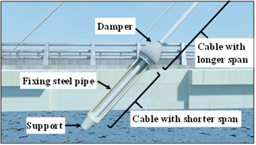
FIGURE 2. A computer-generated image of a cable with a damper.

If the damping effect is large and the cable is hit on the longer span, the damper will absorb the vibration, and it may be difficult for the vibration to be transmitted to the shorter span. Therefore, it is difficult to excite the dominant vibration mode on the shorter span by hitting the cable on the longer span. Additionally, it is also difficult for the dominant vibration mode on the shorter span to be transmitted to the longer span because the damper absorbs the vibration; therefore, this mode is far difficult to measure using accelerometers installed on the longer span.

Hence, if the natural frequencies of certain modes cannot be detected, the wrong modal order is assigned to the measured natural frequencies. Therefore, a new method that does not require the modal order to be specified is needed.

Furthermore, to assign a modal order to each natural frequency in Eq. 26, the previously proposed method has to solve ${\overline{\theta }}_i$ in Eq. 25. Because Eq. 25 has infinite number of solutions, ${\overline{\theta }}_i$ is limited in the range of $(0, \pi$), assuming that the increase in natural frequencies caused by the damper is not large. However, there is no guarantee that this assumption can always be satisfied. Therefore, a new method that does not require the modal order to be specified, that is, it does not require Eq. 25 to be solved, is needed.

3 Proposed Methods for Cable Tension Estimation (Methods 1F and 2F)

3.1 Proposed Method for Cable Tension Estimation Considering Imaginary Part of Complex Natural Frequencies (Method 1F)

3.1.1 Concept of Considering the Imaginary Part of a Complex Natural Frequency

This section presents a modified method (Method 1F), which does not ignore the imaginary part of the complex natural frequency.

The i^th mode complex natural frequency $f_i^t$ can be written using $H_i$, as follows:

$f_i^t=Re\left(f_i^t\right)\left(1+j\frac{Im\left(f_i^t\right)}{Re\left(f_i^t\right)}\right)=Re\left(f_i^t\right)\left(1+j{H}_i\right)(28)$

where $H_i$ is defined as the ratio of the imaginary part to the real part of the complex natural frequency; $H_i$ is also defined as the ratio between the logarithmic decrement of the $i$^th mode ${\delta }_i$ to $2\pi$ ($H_i={\delta }_i/2\pi$), and is also related to the damping factor $h_i$ of the $i$^th mode ($H_i=h_i/\sqrt{1-h_i^2}$).

Because it is difficult to obtain $H_i$ through measurements, this study considered $H_i$ as an unknown. Because the number of unknowns increases when $H_i$ is considered an unknown, the number of constraint equations should also increase. This study uses the additional constraint equation wherein the ratio of the imaginary part to the real part of the complex natural frequency is equal to $H_i$.

3.1.2 Procedure for Estimating Cable Tension From Natural Frequencies

The proposed method inversely estimates $T$, $EI$, $k_u$, $k_v$, and $H_i$ for the high-damping rubber damper, or $T$, $EI$, $k$, $c$, and $H_i$ for the viscous shear damper, from $\rho$, $A$, $L, i$, and the measured natural frequency $f_i^m$ of the $i$^th mode.

The procedure is summarized as follows. It is assumed that $n$ sets of natural frequencies $f_i^m$ have been measured. The complex natural frequency $f_i^t$ can be computed using Eqs. 29–33, and is the function of $4+n$ parameters ($T$, $EI$, $k_u$, $k_v$, and $H_i$, or $T$, $EI$, $k$, $c$, and $H_i$). Then, the optimization problem in Eq. 34 can be solved to simultaneously estimate these $4+n$ parameters. The two constraint equations for the real and imaginary parts of the natural frequency are used.

${\alpha }_i=\sqrt{\sqrt{{\left(\frac{T}{2EI}\right)}^2+\frac{\rho A{\left(2\pi f_i^m\left(1+j{H}_i\right)\right)}^2}{EI}}-\frac{T}{2EI}}(29)$

${\beta }_i=\sqrt{\sqrt{{\left(\frac{T}{2EI}\right)}^2+\frac{\rho A{\left(2\pi f_i^m\left(1+j{H}_i\right)\right)}^2}{EI}}+\frac{T}{2EI}}(30)$

$k_i^{\ast }=\{\begin{array}{cc}{k}_u+j{k}_v& \left(\text{high}-\text{damping}\text{rubber}\text{damper}\right)\\ k+j\left(2\pi f_i^m\left(1+j{H}_i\right)\right)c& \left(\text{viscous}\text{shear}\text{damper}\right)\end{array}(31)$

${\theta }_i={\text{tan}}^{-1}\frac{\frac{k_i^{\ast }}{EI}\frac{{\text{sin}}^2{\alpha }_i{L}_1}{{\alpha }_i}}{{\alpha }_i^2+{\beta }_i^2+\frac{k_i^{\ast }}{EI}\left(\frac{\text{sin}{\alpha }_i{L}_1\text{cos}{\alpha }_i{L}_1}{{\alpha }_i}-\frac{\text{sinh}{\beta }_i{L}_1\text{sinh}{\beta }_i{L}_2}{{\beta }_i\text{sinh}{\beta }_{i}L}\right)}(32)$

$f_i^t=\sqrt{\frac{{\pi }^{2}EI}{4\rho A{L}^4}{\left(i+\frac{{\theta }_i}{\pi }\right)}^4+\frac{T}{4\rho A{L}^2}{\left(i+\frac{{\theta }_i}{\pi }\right)}^2}i=\mathrm{1,2},\dots (33)$

$minimize{G}_1\left(T,EI,k_u,k_v,H_i\right)={\displaystyle \sum }_{i=1}^n\left\{{\left(\frac{\text{Re}\left(f_i^t\right)}{f_i^m}-1\right)}^2+{\left(\frac{\text{Im}\left(f_i^t\right)}{f_i^m}-H_i\right)}^2\right\}\left(\text{high}-\text{damping}\text{rubber}\text{damper}\right)(\mathrm{34a})$

$minimize{G}_1\left(T,EI,k,c,H_i\right)={\displaystyle \sum }_{i=1}^n\left\{{\left(\frac{\text{Re}\left(f_i^t\right)}{f_i^m}-1\right)}^2+{\left(\frac{\text{Im}\left(f_i^t\right)}{f_i^m}-H_i\right)}^2\right\}\left(\text{viscous}\text{shear}\text{damper}\right)(\mathrm{34b})$

Because $n$ is the number of natural frequencies, there are $4+n$ unknowns, namely, $T$, $EI$, $k_u$, $k_v$, and $H_i$, or $T$, $EI$, $k$, $c$, and $H_i$. In contrast, there are $2n$ constraint equations. Therefore, $n$ must at least be equal to four. In the new method (Method 1F), the number of the required natural frequencies is the same as that in the previously proposed method (Method 0F).

3.2 Proposed Cable Tension Estimation Method Considering Imaginary Part of Complex Natural Frequencies Without Specifying Modal Order (Method 2F)

3.2.1 Concept of Method That Does Not Require Specifying the Modal Order

This section proposes a modified method (Method 2F), which does not ignore the imaginary part of the complex natural frequency and does not require the modal order to be specified. The idea behind not specifying the modal order is to use Eq. 11 instead of Eq. 15. The left-hand side of Eq. 11 is rewritten using $i$ as the modal order, and a new function $g_i$ for the $i$^th mode is defined as follows:

$g_i\equiv \text{sin}{\alpha }_{i}L\left\{{\alpha }_i^2+{\beta }_i^2+\frac{k_i^{\ast }}{EI}\left(\frac{\text{sin}{\alpha }_i{L}_1\text{cos}{\alpha }_i{L}_1}{{\alpha }_i}-\frac{\text{sinh}{\beta }_i{L}_1\text{sinh}{\beta }_i{L}_2}{{\beta }_i\text{sinh}{\beta }_{i}L}\right)\right\}-\text{cos}{\alpha }_{i}L\left(\frac{k_i^{\ast }}{EI}\frac{{\text{sin}}^2{\alpha }_i{L}_1}{{\alpha }_i}\right)(35)$

Because Eq. 35 does not explicitly include the modal order $i$, a method that does not require using the modal order can be developed.

3.2.2 Procedure for Estimating Cable Tension From Natural Frequencies

The procedure is summarized as follows. It is assumed that $n$ sets of natural frequencies $f_i^m$ have been measured. The function $g_i$ in terms of $4+n$ parameters ($T$, $EI$, $k_u$, $k_v$, and $H_i$, or $T$, $EI$, $k$, $c$, and $H_i$) is computed using Eqs. 29–31, 35. Then, the optimization problem in Eq. 36 is solved to simultaneously estimate the $4+n$ parameters. The two constraint equations for the real and imaginary parts of $g_i$ are used.

$minimize{G}_2\left(T,EI,k_u,k_v,H_i\right)={\displaystyle \sum }_{i=1}^n\left\{{\left(\text{Re}\left(g_i\right)\right)}^2+{\left(\text{Im}\left(g_i\right)\right)}^2\right\}\left(\text{high}-\text{damping}\text{rubber}\text{damper}\right)(\mathrm{36a})$

$minimize{G}_2\left(T,EI,k,c,H_i\right)={\displaystyle \sum }_{i=1}^n\left\{{\left(\text{Re}\left(g_i\right)\right)}^2+{\left(\text{Im}\left(g_i\right)\right)}^2\right\}\left(\text{viscous}\text{shear}\text{damper}\right)(\mathrm{36b})$

Because $n$ is the number of natural frequencies, there are $4+n$ unknowns, namely, $T$, $EI$, $k_u$, $k_v$, and $H_i$, or $T$, $EI$, $k$, $c$, and $H_i$. In contrast, there are $2n$ constraint equations. Therefore, $n$ must at least be equal to four. The number of necessary natural frequencies of the new method (Method 2F) is the same as that of the other two methods (Methods 0F and 1F).

Method 2F improves two points, namely, ignoring the imaginary part of the complex natural frequencies and the necessity of specifying the modal order. Among the three methods, Method 2F is only appropriate when it is difficult to specify the modal order correctly for each natural frequency. Notably, Method 1F is advantageous over Method 2F when it is possible to specify the modal order correctly, because Method 1F uses more information (both the natural frequencies and modal order) for estimation.

The comparison of the three methods is presented in Table 1.

TABLE 1

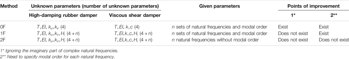
TABLE 1. A comparison of three tension estimation methods ($i$ is the modal order and $n$ is the number of natural frequencies).

3.3 MultiStart Algorithm

All methods solve the nonlinear least squares problem. Therefore, there may be multiple local minimum solutions, although the global minimum solution is preferable. The solution depends on the initial points (initial parameters for unknowns). Therefore, this study used the MultiStart algorithm (MathWorks, 2020), wherein the solver attempts to find multiple local minima solutions to a problem by starting from various initial points. The final solution is the one with the best objective function value among the local minimum solutions. Although there is no guarantee that this algorithm will always find the global minimum solution, it can still find a better solution than the general nonlinear least squares method using only one starting point.

4 Numerical Verification

4.1 Overview

The validity of the proposed method was verified by numerical simulation. First, the values of the cable parameters ($\rho$, $A$, $L, L_1, T,$ and $EI$) and damper parameters ($k_u$ and $k_v$, or $k$ and $c$) were assumed. Next, the natural frequencies of the cable with a damper, which are the real parts of the theoretical complex natural frequencies $\text{Re}\left(f_i^t\right)$, were calculated from Eqs. 17–21. Then, the calculated natural frequencies were input into the proposed methods to estimate $T$, $EI$, $k_u$, $k_v$, and $H_i$, or $T$, $EI$, $k$, $c$, and $H_i$. The estimation accuracy was investigated by comparing the estimated values to the assumed values.

4.2 Analytical Conditions

4.2.1 Analytical Cases

The cable parameters are listed in Table 2A, and the damper parameters are listed in Table 2B. These values were set to cover a wide range of cables and dampers. In practical situations, the damper is installed near the girder. Therefore, the damper location, $L_1$, was set to a small value compared with the cable length, $L$.

TABLE 2

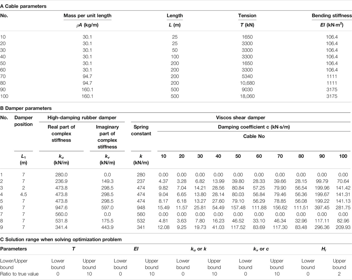
TABLE 2. Analytical parameters.

The two damper types, namely, the high-damping rubber damper and a viscous shear damper, were compared.

For the high-damping rubber damper, the values of the real part $k_u$ and the imaginary part $k_v$ of the complex stiffness $k_i^{\ast }$ are listed in Table 2B.

For the viscous shear damper, the spring constant $k$ was set to the same value as $\left|k_i^{\ast }\right|$ of the high-damping rubber damper. The damping coefficient $c$ was determined such that the imaginary part of the first mode complex stiffness $\text{Im}(k_1^{\ast }$) becomes similar for the two damper models. To be more concrete, the damping coefficient $c$ was determined by $c=k_v/2\pi f_1$ where $f_1$ is the first mode natural frequency of a cable with a high-damping rubber damper in the same damper case. The values of $k$ and $c$ are listed in Table 2B.

By combining ten cable models and nine damper models, 90 numerical models were established in total. The model number is defined as the sum of the cable number and damper number. For example, the analytical model No. 15 consists of cable model No. 10 and damper model No. 5.

4.2.2 Number of Natural Frequencies Used in Estimation

At least four natural frequencies are required to estimate the unknowns. Based on the authors’ previous experience on measuring the natural frequencies of a cable with a damper, it is known that there are cases wherein the natural frequencies can be measured only up to the seventh mode (Furukawa et al., 2021b). The natural frequencies of the higher modes are occasionally difficult to measure because the higher-mode vibration is rapidly dissipated by the dampers. Therefore, the natural frequencies of the first seven modes were used to estimate the unknowns.

4.2.3 Solving Nonlinear Optimization

The MultiStart algorithm with the nonlinear least-squares method was used to estimate the unknowns. The estimation accuracy depends on the number of initial points and the lower and upper bounds of each unknown. This study randomly generated 200 sets of initial points for unknowns to avoid a local minimum solution. Table 2C indicates the lower and upper bounds of the unknowns when searching for solutions.

4.3 Estimation Results

The first-mode to seventh-mode natural frequencies of 90 models were input into the proposed methods, and the unknowns were estimated. In Methods 0F and 1F, the modal order was also input. For Method 0F, four unknowns, namely, $T$, $EI$, $k_u$, and $k_v$ for the high-damping rubber damper, or $T$, $EI$, $k$, and $c$ for the viscous shear damper, were estimated. Methods 1F and 2F estimate 11 unknowns, namely, $T$, $EI$, $k_u$, $k_v$, and $H_i$ ($i$ = 1, … ,7) for the high-damping rubber damper, or $T$, $EI$, $k$, $c$, and $H_i$ ($i$ = 1, … ,7), for the viscous shear damper.

The results estimated for the high-damping rubber damper are shown in Figure 3. The estimated results for the viscous shear damper are shown in Figure 4. The horizontal axis is the model number. The vertical axis is the ratio of the estimated value to the true (assumed) value. Notably, a model whose vertical axis value is closer to 1.0 has a higher estimation accuracy.

FIGURE 3

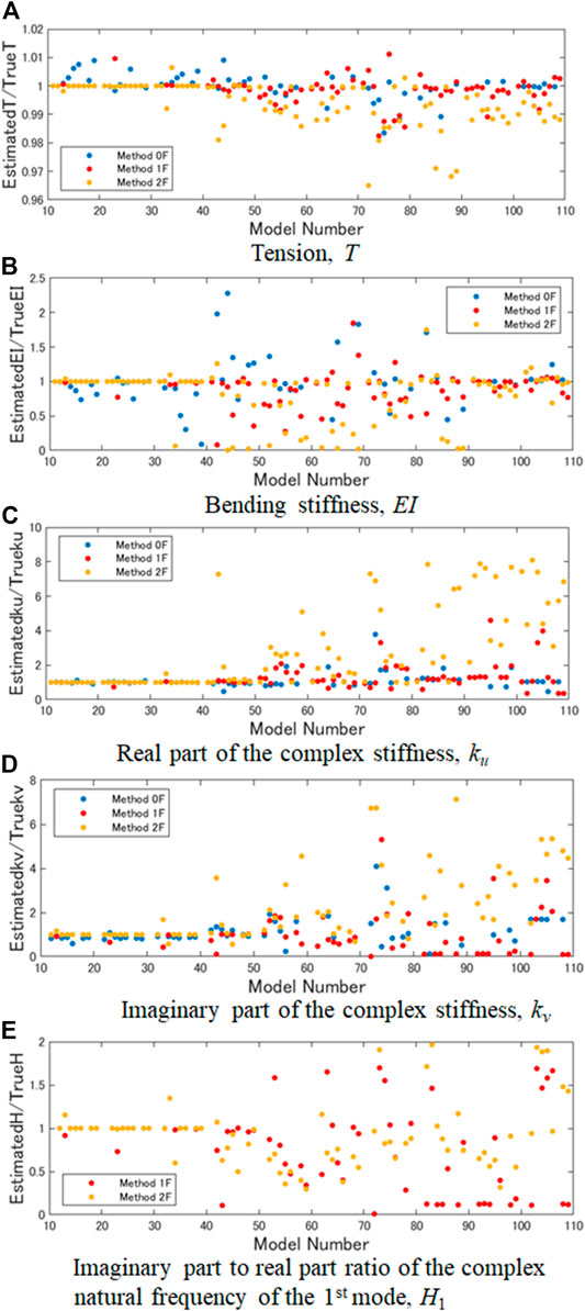
FIGURE 3. Estimation results for a cable with a high-damping rubber damper: (A) tension, T; (B) bending stiffness, EI; (C) real part of complex stiffness, k_u; (D) imaginary part of complex stiffness, k_v; (E) imaginary part to real part ratio of complex natural frequency of 1^st mode, H₁.

FIGURE 4

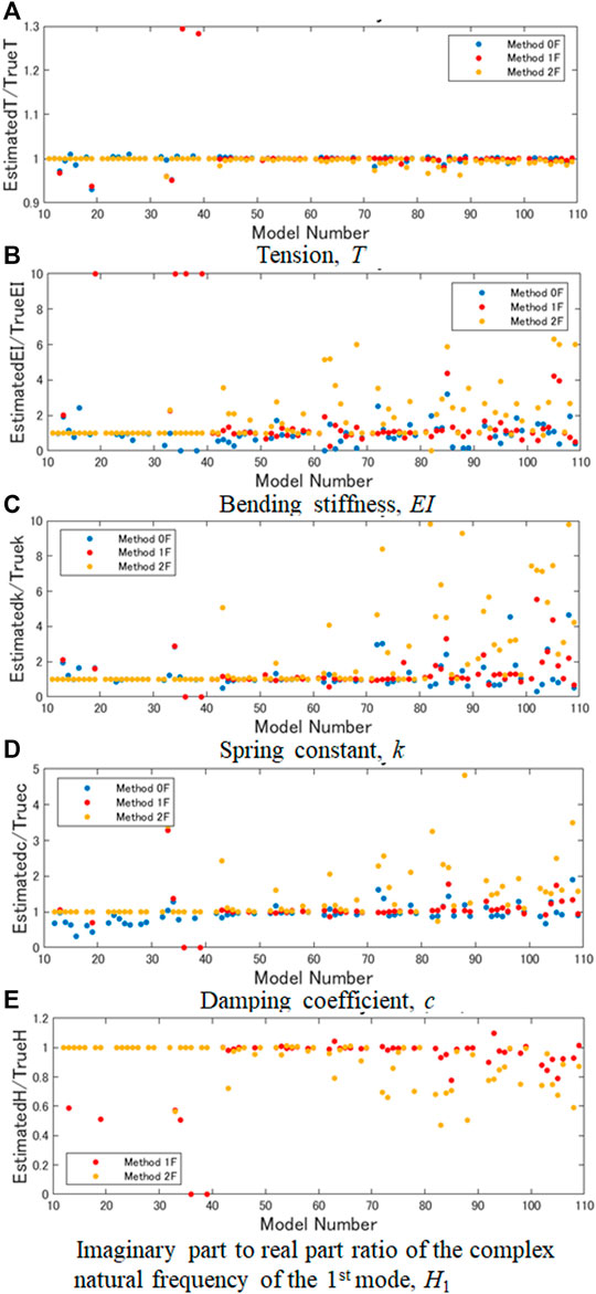
FIGURE 4. Estimation results for a cable with a viscous shear damper: (A) tension, T; (B) bending stiffness, EI; (C) spring constant, k; (D) damping coefficient, c; (E) imaginary part to real part ratio of complex natural frequency of 1^st mode, H₁.

4.3.1 Results of Tension Estimation

Previous studies have reported that the tension estimation error of the higher-order vibration method is 5% for a cable without a damper (Shinko Wire Company, Ltd, 2020). Therefore, the target tension estimation error for a cable with a damper was set to 5% in this study.

4.3.1.1 High-Damping Rubber Damper

The result of tension estimation for a cable with a high-damping rubber damper is shown in Figure 3A. Methods 0F, 1F, and 2F are indicated by blue, red, and yellow dots, respectively. When the blue and red dots cannot be seen, they overlap the yellow dot. When only the red dot cannot be seen, it overlaps the yellow dot. When only the blue dot cannot be seen, it overlaps the red or yellow dots.

The range of the vertical axis was 0.96–1.02. For all methods, the estimation error was within 4%. The high estimation accuracy was confirmed for tension, and the target error of 5% was achieved.

Next, the three methods are compared in terms of tension estimation accuracy. For models No. 11 to 49, when the cable was shorter than or equal to 100 m, the estimation accuracy of Method 0F was the lowest. For models No. 51 to 109, when the cable was longer than or equal to 200 m, the estimation accuracy of Method 0F was the highest. The reason for this is as follows. For models No. 11 to 49 with a shorter cable, the effect of damping became large. Therefore, ignoring the imaginary part of the complex natural frequency of Method 0F deteriorates the tension estimation accuracy. For models No. 51 to 109 with a long cable, the effect of damping is not large. Therefore, ignoring the imaginary part of the complex natural frequency of Method 0F does not deteriorate the tension estimation accuracy and improves the tension estimation accuracy because the unknowns of Method 0F are fewer than those of Methods 1F and 2F.

Next, the tension estimation accuracy of Methods 1F and 2F is compared. Method 1F uses the natural frequencies and their modal orders as a set, while Method 2F only uses natural frequencies and does not use the modal order. In this numerical verification, the modal order was correctly assigned. Therefore, Method 1F has more information than Method 2F. Hence, the accuracy of Method 1F is higher than that of Method 2F, particularly for models with a long cable. The tension estimation accuracy of Method 2F is lower than that of Method 1F, but the estimation accuracy is still high.

4.3.1.2 Viscos Shear Damper

The result of tension estimation for a cable with a viscous shear damper is shown in Figure 4A. In most cases, the estimation error was within 5%. However, the estimation error of Methods 0F and 1F was larger than 5% for models No.19, 36, and 39. As presented in Table 2B, these models have a short cable and large damping coefficient. This indicates that the models with large estimation errors have high natural frequencies for higher modes and a large damping coefficient. If the natural frequency is high and the damping constant is large, the imaginary part of the damper’s complex stiffness $k_i^{\ast }$ is also large.

For this reason, ${\overline{\theta }}_i$ and ${\theta }_i$ of models No. 19, 36, and 39 exceed $\pi$, and the limitation of ${\overline{\theta }}_i$ and ${\theta }_i$ in the range of $\left(0, \pi \right)$ has a deteriorating effect on the tension estimation accuracy.

Method 2F could estimate the tension accurately for model No. 19, 36, and 39 because Method 2F does not require the calculation of ${\theta }_i$ and has no limitation.

4.3.2 Results of Bending Stiffness Estimation

The bending stiffness estimation result for the two damper models is shown in Figures 3B, 4B. The bending stiffness estimation accuracy is low compared with the tension estimation accuracy because only the low frequencies from the first to the seventh modes were used in the estimation. As expressed by Eqs. 26, 33, the sensitivity of the bending stiffness $EI$ over the complex natural frequencies $f_i^t$ is low because the $EI$ coefficient is much smaller than the $T$ coefficient in the lower mode. Therefore, to estimate the bending stiffness with a high accuracy, it is necessary to use higher-order natural frequencies. However, considering that the higher-mode vibration is rapidly dissipated by the damper, it is difficult to measure the higher-mode natural frequencies in practical situations. Therefore, it is concluded that it is difficult to estimate the bending stiffness with high accuracy in actual situations.

4.3.3 Results of Damper Parameter Estimation

The damper parameter estimation result for the two damper models is shown in Figures 3C,D, 4C,D. Satisfactory accuracy, such as that of tension estimation, is difficult to achieve in damper parameter estimation because the $k_i^{\ast }$ value is not independent of the bending stiffness $EI$, as follows from Eqs. 25, 32. The $k_i^{\ast }/EI$ ratio is an independent parameter; therefore, the accuracy of the damper parameter estimation depends on the accuracy of bending stiffness estimation. Because the bending stiffness estimation accuracy is not high, the accuracy of the damper parameters is also not high.

A comparison between the results shown in Figures 3D, 4D reveals that the estimation accuracy of $c$ is better than that of $k_v$, particularly when the cable is short (the model number is small). The sensitivity of the imaginary part of the damper stiffness is higher for a short cable with a viscous shear damper.

4.3.4 Results of Estimation of Imaginary Part to Real Part Ratio of Complex Natural Frequency

The estimation result for the imaginary part to the real part ratio of the first mode complex natural frequency, $H_1$, is shown in Figures 3E, 4E. The results for higher modes exhibited a tendency similar to that of the first mode. The accuracy deteriorates as the cable length increases because the effect of the damper decreases as the cable length increases. Therefore, it is difficult to achieve a satisfactory accuracy such as that of tension estimation.

The accuracy with the viscous shear damper in Figure 4E is better than that with the high-damping rubber damper in Figure 3E, for the same reason that the estimation accuracy for $c$ is higher than that for $k_v$.

4.4 Effect of Measurement Error on Tension Estimation Accuracy

4.4.1 Analytical Condition

When measuring the acceleration of an actual bridge cable, the natural frequencies always contain measurement error. Therefore, this section discusses the effect of measurement error on the tension estimation accuracy. Artificial measurement error was added to the natural frequencies calculated by eigenvalue analysis. The natural frequencies with measurement error were calculated as follows according to the approach used by Thyagarajan et al. (1998).

$f_i^{noise}=\left(1+\eta rand\right)\text{Re}\left(f_i^t\right)i=1, 2,\dots (37)$

where $f_i^t$ denotes the natural frequencies of the $i$ ^th mode calculated by eigenvalue analysis, $\eta$ is the measurement error ratio, and $rand$ is a uniform random number between −1 and 1. The measurement error ratio $\eta$ = 0.02 was used.

The tension, bending stiffness, and damper parameters were estimated using Methods 0F, 1F, and 2F by inputting natural frequencies with measurement error. Because the bending stiffness and damper parameter estimation accuracy is not satisfactory, even in the case without measurement error, only the accuracy of estimating tension was investigated.

4.4.2 Results

Because the estimation accuracy depends on the combination of random numbers generated for each natural frequency, the average value of ten sets of natural frequencies with measurement error was used for the estimation by iterating the calculation of Eq. 37 10 times.

The tension estimation results for a cable with a high-damping rubber damper and a viscos shear damper are shown in Figure 5.

FIGURE 5

FIGURE 5. Tension estimation results for cases with measurement error: (A) high-damping rubber damper; (B) viscos shear damper.

For the high-damping rubber damper, model No. 23 had the largest maximum error among all methods. The largest maximum error of Method 0F, Method 1F, and Method 2F is 0.081, 0.094, and 0.073, respectively. The maximum error of Method 2F is the smallest, but the difference among the three methods is small.

For the viscos shear damper, model No. 36 had the largest maximum error for Methods 0F and 1F (0.295). Method 2F had the smallest maximum error of 0.073 with model No. 41.

Next, the root mean squares error ratio (RMSER) expressed by Eq. 38 was calculated for each method.

$\text{RMSER}=\sqrt{\frac{1}{90}{\displaystyle \sum }_{i=1}^{90}{\left(T_i^{estimated}/T_i^{true}-1\right)}^2}(38)$

Here, $i$ is the model number, $T_i^{estimated}$ is the estimated tension of model number $i$, and $T_i^{true}$ is the assumed true tension of model number $i$.

The calculated RMSER is presented in Table 3. For comparison, the values in the cases without measurement error (the measurement error ratio is 0.0) and cases with measurement error (the measurement error ratio is 0.02) are shown. The RMSER increased owing to the measurement error, regardless of the damper type and the method used.

TABLE 3

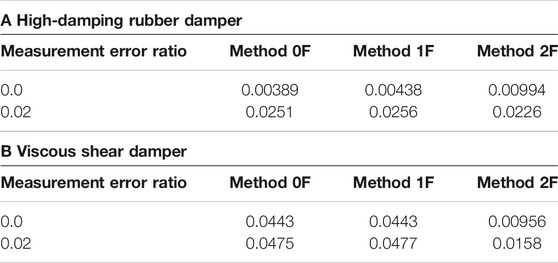
TABLE 3. RMSER of tension estimation.

For the high-damping rubber damper, Method 2F had the smallest RMSER but the difference among the three methods is very small.

For the viscos shear damper, Method 2F had the smallest RMSER, even in the case wherein the measurement error was 0.02, because no assumptions nor limitations exist in Method 2F, as already explained in Section 4.3.1.2.

4.5 Summary

In this section, the validity of Methods 0F, 1F, and 2F was numerically verified. The tension estimation accuracy is high, but the estimation accuracy of the other parameters is low.

First, the comparison between methods 0F and 1F is summarized. Method 0F ignores the imaginary part of the complex natural frequencies and requires the estimation of four unknowns. Method 1F does not ignore the imaginary part of the complex natural frequencies and recognizes them as unknowns, and thereby has more unknowns to estimate compared with Method 0F. In the case of short cables, the effect of the damper and the effect of the imaginary part of the complex frequency are relatively large. Therefore, Method 1F achieves a higher accuracy. However, in the case of long cables, the effect of the damper is not large; therefore, ignoring the complex frequency is acceptable. Thus, Method 0F with fewer unknowns achieves a higher accuracy compared with Method 1F with more unknowns.

Next, the comparison among the three methods is summarized. In most models, the tension estimation error was within 5%, regardless of the method used. However, when the cable had high natural frequencies and the viscous shear damper had a large damping coefficient, the tension estimation error of Methods 0F and 1F was larger than 5% because the assumption was not satisfied. In these cases, the estimation error of Method 2F was within 5% because no assumptions nor limitations exist in Method 2F.

The effect of the measurement error on the tension estimation accuracy was also investigated. Method 2F had the smallest estimation error (maximum error and RMSER), particularly when the viscos shear damper was used.

Based on the above-mentioned findings, this study concluded that Method 2F is the most versatile among the three methods.

5 Experimental Verification

5.1 Experimental Condition

This section describes the experimental validation of the proposed methods. The experimental setting is shown in Figure 6A. The experiment was conducted using a horizontal cable with a length of 61.8 m. The distance between the two ends was considered equal to the cable length. A load cell was installed at the right end, and the tension value of the load cell was considered the true tension value. The cable was hit with a hammer between the damper position and the right end. Additionally, the acceleration histories were measured by accelerometers. The natural frequencies were measured by reading the peak frequencies of the acceleration Fourier spectra.

FIGURE 6

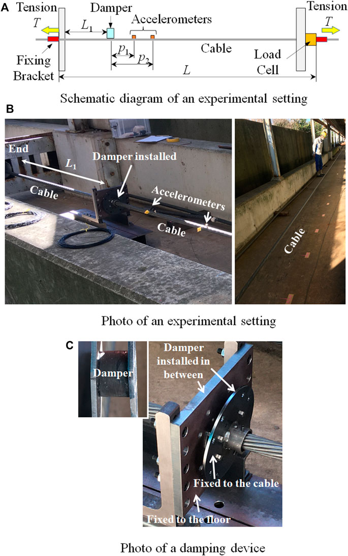
FIGURE 6. Experimental setting: (A) schematic diagram of experimental setting; (B) photograph of experimental setting; (C) photograph of damping device.

Figure 6B shows a photograph of the experimental setting. The damper was placed at a distance $L_1$ from one end. Piezoelectric accelerometers were magnetically attached to the cable. A compression load cell was used, but the photograph of the load cell is not shown here.

Figure 6C shows a photograph of the damper device. A rectangular steel plate with a circular hole for the cable to pass through was fixed to the floor. The cable was not in contact with the steel plate. A disk-shaped steel plate with a circular hole for the cable to pass through was fixed to the cable. The damper was installed between the rectangular steel plate and the disk-shaped steel plate. The rectangular steel plate and the disk-shaped steel plate were installed parallel to each other. The damper shown in Figure 6C exerted a stiffness and damping effect.

The cable parameters are presented in Table 4. A prestressed steel strand was used as the cable because it is used in actual bridge cables.

TABLE 4

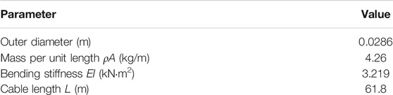
TABLE 4. Cable parameters.

The damper parameters are listed in Table 5. Three high-damping rubber dampers were used.

TABLE 5

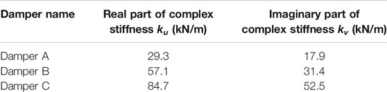
TABLE 5. Damper parameters estimated by element test.

The test cases are listed in Table 6. Cases No. 1 to No. 13 involve tension of approximately 180 kN. Cases No. 14 to No. 26 involve tension of approximately 380 kN. Cases No. 1 and No. 14 are cases without a damper. Regarding the damper position, four cases were considered for each tension and damper combination.

TABLE 6

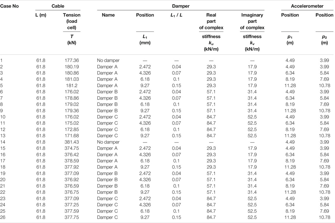
TABLE 6. Test cases.

To solve the optimization problem using the MultiStart algorithm, this study randomly generated 200 sets of initial points for the unknowns to avoid a local minimum solution. Table 7 presents the lower and upper bounds of the unknowns in the search for solutions. The lower bounds were set to zero for all parameters. The upper bound of tension was set to ten times the true value. The upper bound of the bending stiffness was set to ten times the design value. The upper bounds of the damper parameters were not limited because the damper stiffness has amplitude-dependency and frequency-dependency. The damper parameters during the vibration test are considered to be different to the values obtained during an element test (Table 5). Regarding the imaginary part to the real part ratio of the complex natural frequencies, the upper value was set to 0.019. The damping factor of each mode was evaluated using the half-power method, and 0.019 was set as the upper bound.

TABLE 7

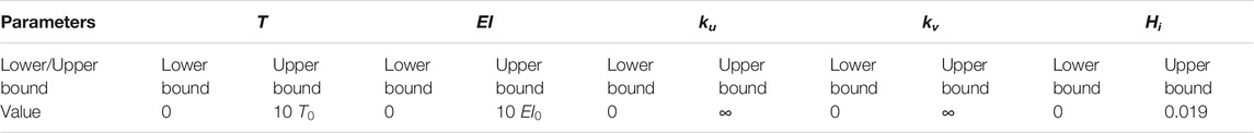
TABLE 7. Solution range when solving optimization problem ($T_0$: tension measured by load cell in Table 5C; $E{I}_0$: design value in catalog listed in Table 5A).

Table 8 lists the first to seventh measured natural frequencies, for which the order was assigned in an ascending order based on the measured peak frequencies.

TABLE 8

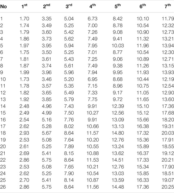
TABLE 8. First to seventh measured natural frequencies in ascending order (Hz).

5.2 Tension Estimation Results

The measured natural frequencies and their orders listed in Table 8 were input into Methods 0F and 1F, and only the measured natural frequencies were input into Method 2F. Because the accuracy of estimating parameters other than tension is not satisfactory, as discussed in the previous section, only the tension estimation accuracy is discussed here.

Figure 7 shows the estimation results for tension. The horizontal axis is the case number, and the vertical axis is the ratio of the estimated tension to the true tension measured by a load cell.

FIGURE 7

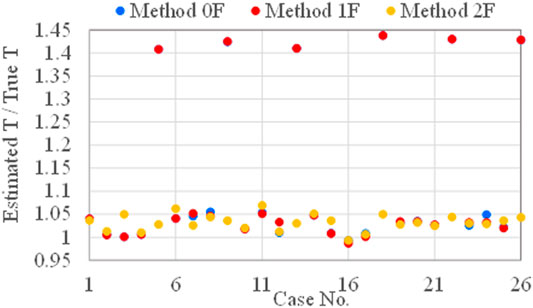
FIGURE 7. Tension estimation results.

The vertical axis for Method 2F is between 0.993 and 1.069. The estimation error of Method 2F for cases No. 6 and 11 exceeds 5%, but Method 2F has the highest accuracy among the three methods.

The vertical axis for Methods 0F and 1F is larger than 1.4 for case No. 5, 9, 13, 18, 22, and 26. These are cases wherein the damper is installed furthest from the edge ($L_1/L$ is 0.15). To determine why the accuracy of Methods 0F and 1F is unsatisfactory when the damper is installed far from the edge, the measured natural frequency was compared with the theoretical natural frequencies. Table 9 presents the comparison between the measured and theoretical natural frequencies. The theoretical natural frequencies are the real parts of the theoretical complex natural frequencies $\text{Re}\left(f_i^t\right)$, and were calculated using Eqs. 17–21 with the cable and damper parameters listed in Table 4 and Table 5. From Table 9, two conclusions can be drawn. First, the measured natural frequencies are slightly different to the theoretical values. The reason for this is that the actual damper stiffness is different to the value in Table 5, which was estimated by an element test because the actual damper is amplitude-dependent and frequency-dependent. Second, the natural frequency of the fifth mode was not detected in the experiment. Therefore, the modal order was fixed by skipping the fifth mode, as presented in Table 9. The fifth mode is the mode wherein the vibration in the shorter span with a length of $L_1$ is dominant. The cable was excited using a hammer at the longer span, and the damper dissipated the vibration. Therefore, the fifth mode that is dominant in the shorter span was difficult to excite. Moreover, the acceleration responses were only measured at the longer span. For these reasons, the fifth mode was not generated, or could not be detected because its amplitude was too small.

TABLE 9

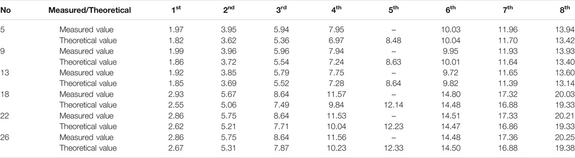
TABLE 9. Comparison between measured and theoretical natural frequencies (Hz).

In the cases wherein the damper was installed near the edge ($L_1/L$ is 0.04, 0.07, and 1.0), the modal order wherein the vibration of the shorter span was dominant was higher than the seventh mode. For this reason, the estimation accuracy of Methods 0F and 1F was as high as that of Method 2F in these cases.

5.3 Tension Estimation Results After Fixing Modal Order

The modal order of cases No. 5, 9, 13, 18, 22, and 26 was fixed, as presented in Table 9. Then, the tension was estimated again using Methods 0F and 1F. The results are shown in Figure 8. Only the results for cases No. 5, 9, 13, 18, 22, and 26 for Methods 0F and 1F are replaced with those in Figure 7.

FIGURE 8

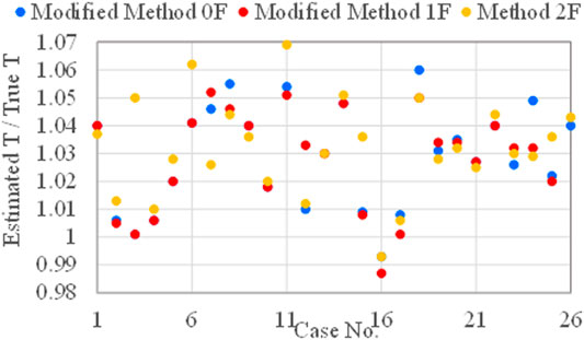
FIGURE 8. Tension estimation results after fixing modal order.

The vertical axis was between 0.993 and 1.06 for Method 0F, between 0.987 and 1.052 for Method 1F, and between 0.993 and 1.069 for Method 2F. The maximum estimation error was 6.0% for Method 0F, 5.2% for Method 1F, and 6.9% for Method 2F. If the modal order was correctly assigned, Method 1F had the highest accuracy because the high-damping rubber damper instead of the viscous shear damper was used in the experiment. In practical cases, however, it is not always possible to fix the modal order because it is typically difficult to obtain the design values of tension and bending stiffness, and the damper parameters of the actual structures in advance. Therefore, Method 2F is considered to be an efficient method that does not limit the target structures.

In future work, the authors will improve Method 2F to achieve an estimation error within 5%.

6 Conclusion

This study improved a previously proposed method for estimating the tension of a cable with a damper. The previously proposed method (Method 0F) estimates the cable’s tension, cable’s bending stiffness, and damper parameters based on the natural frequencies and their modal order. In Method 0F, there are two points of improvement. First, Method 0F partially ignores the imaginary part of complex natural frequencies. Second, Method 0F needs both the natural frequencies and their modal order as a set. In this study, Methods 1F and 2F are proposed to improve the above-mentioned points. Method 1F improves the first point, while Method 2F improves both points.

First, the validity of the proposed methods was numerically verified. Two damper types, namely, a high-damping rubber damper and a viscous shear damper, were considered. Ninety numerical models were established with ten cable models and nine damper models for each damper type.

The cable tension was estimated with high accuracy. However, the other parameters, namely, the bending stiffness of the cable, the two damper parameters, and the imaginary part to the real part ratio of the complex natural frequencies, were difficult to estimate with high accuracy.

In most models, the tension estimation error was within 5% regardless of the method used. However, when a cable with high natural frequencies and a viscous shear damper with a large damping coefficient were used, the tension estimation accuracy of Methods 0F and 1F was low owing to the second point of improvement. Method 2F is the only method that accurately estimated the cable tension, and its estimation error was less than 5% in all cases.

The effect of the measurement error on the tension estimation accuracy was also investigated. Method 2F had the smallest estimation error (maximum error and RMSER), particularly when the viscos shear damper was used.

Next, the validity of the proposed methods was experimentally verified using a cable with a length of 61.8 m. A high-damping rubber damper was installed. A total of 26 cases were prepared by changing the cable tension, damper models, and damper position. The modal order of the natural frequencies was specified in an ascending order.

Among the three methods, the accuracy of Method 2F was the highest, and the maximum estimation error was 6.9%. The tension estimation error of Methods 0F and 1F became larger than 40% when the distance between the damper position and the nearest cable end was 0.15 times equal to the cable length. The fifth mode, whose vibration is dominant in the cable’s shorter span, was not detected, and the modal order of the observed natural frequencies was erroneously assigned. The accuracy degradation caused by the second point of improvement occurred in Methods 0F and 1F. By fixing the modal order, the tension could be estimated with high accuracy by Methods 0F and 1F. However, it is not always possible to fix the modal order in practice. Therefore, Method 2F is an efficient method that does not limit the target structures.

The numerical and experimental verifications clearly demonstrate the superiority of Method 2F, and it is possible to estimate the cable tension without detaching the damper. The fact that the cable does not have to be detached is a great advantage in terms of work efficiency.

In the engineering practice, there is a problem that the natural frequencies of the higher modes are occasionally difficult to measure because the higher-mode vibration is rapidly dissipated by the dampers. Based on the authors’ previous experience on measuring the natural frequencies of a cable with a damper in a real cable-stayed bridge, there are cases wherein the natural frequencies can be measured only up to the seventh mode (Furukawa et al., 2021b). Therefore, the natural frequencies of the first seven modes were used in this study. Since the proposed methods only require four natural frequencies, which are smaller than the seven natural frequencies, they are applicable to the actual engineering problems. In the engineering practice, measurement error is also a problem since it decreases the estimation accuracy. The development of a highly accurate estimation method for the natural frequencies is also a necessary research issue.

In future work, the authors will improve the tension estimation accuracy. Furthermore, verification will be carried out using measurement data obtained for actual bridges.

Data Availability Statement

The original contributions presented in the study are included in the article, further inquiries can be directed to the corresponding author.

Author Contributions

AF developed the proposed methods, wrote the source code for estimating the cable tension, and carried out the numerical analysis. SS carried out the numerical analysis. RK conducted the verification experiment.

Conflict of Interest

Author RK was employed by the Kobelco Wire Company, Ltd.

The remaining authors declare that the research was conducted in the absence of any commercial or financial relationships that could be construed as a potential conflict of interest.

Publisher’s Note

All claims expressed in this article are solely those of the authors and do not necessarily represent those of their affiliated organizations, or those of the publisher, the editors and the reviewers. Any product that may be evaluated in this article, or claim that may be made by its manufacturer, is not guaranteed or endorsed by the publisher.

References

Chen, C.-C., Wu, W.-H., Leu, M.-R., and Lai, G. (2016). Tension Determination of Stay Cable or External Tendon with Complicated Constraints Using Multiple Vibration Measurements. Measurement 86, 182–195. doi:10.1016/j.measurement.2016.02.053

CrossRef Full Text | Google Scholar

Chen, C.-C., Wu, W.-H., Chen, S.-Y., and Lai, G. (2018). A Novel Tension Estimation Approach for Elastic Cables by Elimination of Complex Boundary Condition Effects Employing Mode Shape Functions. Eng. Structures 166, 152–166. doi:10.1016/j.engstruct.2018.03.070

CrossRef Full Text | Google Scholar

Feng, Z., Xiaodong Wang, X., and Zaifa Chen, Z. (2010). “A Method of Fundamental Frequency Hybrid Recognition for cable Tension Measurement of Cable-Stayed Bridges,” in 8th IEEE International Conference on Control and Automation, Xiamen, 9-11 June 2010. doi:10.1109/ICCA.2010.5524186

CrossRef Full Text | Google Scholar

Foti, F., Geuzaine, M., and Denoël, V. (2020). On the Identification of the Axial Force and Bending Stiffness of Stay Cables Anchored to Flexible Supports. Appl. Math. Model. 92, 798–828. doi:10.1016/j.apm.2020.11.043

CrossRef Full Text | Google Scholar

Furukawa, A., Yamada, S., and Kobayashi, R. (2022). Tension Estimation Methods for Two Cables Connected by an Intersection Clamp Using Natural Frequencies. J. Civ. Struct. Health Monit.. doi:10.1007/s13349-022-00548-6

CrossRef Full Text | Google Scholar

Furukawa, A., Hirose, K., and Kobayashi, R. (2021a). Tension Estimation Method for Cable with Damper Using Natural Frequencies. Front. Built Environ. 7, 603857. doi:10.3389/fbuil.2021.603857

CrossRef Full Text | Google Scholar

Furukawa, A., Hirose, K., and Kobayashi, R. (2021b). “Tension Estimation Method for cable with Damper and its Application to Real cable-stayed Bridge,” in Proceedings of the 9th International Conference on Experimental Vibration Analysis for Civil Engineering Structures, (Online), September 15, 2021. Paper No. S8-1.

Google Scholar

Gan, Q., Huang, Y., Wang, R., and Rao, R. (2019). Tension Estimation of Hangers with Shock Absorber in Suspension Bridge Using Finite Element Method. J. Vibroeng. 21 (3), 587–601. doi:10.21595/jve.2018.20054

CrossRef Full Text | Google Scholar

Hou, J., Li, C., Jankowski, Ł., Shi, Y., Su, L., Yu, S., et al. (2020). Damage Identification of Suspender Cables by Adding Virtual Supports with the Substructure Isolation Method. Struct. Control. Health Monit. 28 (3), e2677. doi:10.1002/stc.2677

CrossRef Full Text | Google Scholar

Izzi, M., Caracoglia, L., and Noè, S. (2016). Investigating the Use of Targeted-Energy-Transfer Devices for Stay-Cable Vibration Mitigation. Struct. Control. Health Monit. 23, 315–332. doi:10.1002/stc.1772

CrossRef Full Text | Google Scholar

Javanbakht, M., Cheng, S., and Ghrib, F. (2019). Control-oriented Model for the Dynamic Response of a Damped cable. J. Sound Vibration 442, 249–267. doi:10.1016/j.jsv.2018.10.036

CrossRef Full Text | Google Scholar

Kim, B. H., and Park, T. (2007). Estimation of cable Tension Force Using the Frequency-Based System Identification Method. J. Sound Vibration 304, 660–676. doi:10.1016/j.jsv.2007.03.012

CrossRef Full Text | Google Scholar

Krenk, S. (2000). Vibrations of a Taut Cable with an External Damper. ASME, J. Appl. Mech. 67, 772–776. doi:10.1115/1.1322037

CrossRef Full Text | Google Scholar

Lazar, I. F., Neild, S. A., and Wagg, D. J. (2016). Vibration Suppression of Cables Using Tuned Inerter Dampers. Eng. Structures 122, 62–71. doi:10.1016/j.engstruct.2016.04.017

CrossRef Full Text | Google Scholar

Li, S., Wang, L., Wang, H., Shi, P., Lan, R., Wu, C., et al. (2021). An Accurate Measurement Method for Tension Force of Short cable by Additional Mass Block. Adv. Mater. Sci. Eng. 2021, 1–10. doi:10.1155/2021/6622628

CrossRef Full Text | Google Scholar

Ma, L., Xu, H., Munkhbaatar, T., and Li, S. (2021). An Accurate Frequency-Based Method for Identifying cable Tension while Considering Environmental Temperature Variation. J. Sound Vibration 490, 115693. doi:10.1016/j.jsv.2020.115693

CrossRef Full Text | Google Scholar

Ma, L. (2017). A Highly Precise Frequency-Based Method for Estimating the Tension of an Inclined cable with Unknown Boundary Conditions. J. Sound Vibration 409, 65–80. doi:10.1016/j.jsv.2017.07.043

CrossRef Full Text | Google Scholar

MathWorks (2020). MATLAB Documentation, MultiStart. Available at: https://jp.mathworks.com/help/gads/multistart.html (Accessed April 30, 2021).

Google Scholar

Pacheco, B. M., Fujino, Y., and Sulekh, A. (1993). Estimation Curve for Modal Damping in Stay Cables with Viscous Damper. J. Struct. Eng. 119 (6), 1961–1979. doi:10.1061/(asce)0733-9445(1993)119:6(1961)

CrossRef Full Text | Google Scholar

Shan, D., Zhou, X., and Khan, I. (2019). Tension Identification of Suspenders with Supplemental Dampers for through and Half-Through Arch Bridges under Construction, ASCE. J. Struct. Eng. 145 (3), 04018265. doi:10.1061/(ASCE)ST.1943-541X.0002255

CrossRef Full Text | Google Scholar

Shi, X., and Zhu, S. (2018). Dynamic Characteristics of Stay Cables with Inerter Dampers. J. Sound Vibration 423, 287–305. doi:10.1016/j.jsv.2018.02.042

CrossRef Full Text | Google Scholar

Shinke, T., Hironaka, K., Zui, H., and Nishimura, H. (1980). Practical Formulas for Estimation of Cable Tension by Vibration Method. Proc. Jpn. Soc. Civil Eng. 294, 25–32. (In Japanese). doi:10.2208/jscej1969.1980.294_25

CrossRef Full Text | Google Scholar

Shinko Wire Company, Ltd (2020). Tension Measuring Technique for Outer Cables. Available at: (In Japanese) http://www.shinko-wire.co.jp/products/vibration.html (Accessed April 30, 2021).

Google Scholar

Tabatabai, H., and Mehrabi, A. B. (2000). Design of Mechanical Viscous Dampers for Stay Cables. J. Bridge Eng. 5 (2), 114–123. doi:10.1061/(asce)1084-0702(2000)5:2(114)

CrossRef Full Text | Google Scholar

Thyagarajan, S. K., Schulz, M. J., Pai, P. F., and Chung, J. (1998). Detecting Structural Damage Using Frequency Response Functions. J. Sound Vibration 210, 162–170. doi:10.1006/jsvi.1997.1308

CrossRef Full Text | Google Scholar

Yamagiwa, I., Utsuno, H., Endo, K., and Sugii, K. (2000). Identification of Flexural Rigidity and Tension of the One-Dimensional Structure by Measuring Eigenvalues in Higher Order. Trans.JSME(C) 66649, 2905–2911. (In Japanese). doi:10.1299/kikaic.66.2905

CrossRef Full Text | Google Scholar

Yan, B., Chen, W., Yu, J., and Jiang, X. (2019). Mode Shape-Aided Tension Force Estimation of Cable with Arbitrary Boundary Conditions. J. Sound Vibration 440, 315–331. doi:10.1016/j.jsv.2018.10.018

CrossRef Full Text | Google Scholar

Yan, B., Chen, W., Dong, Y., and Jiang, X. (2020). Tension Force Estimation of Cables with Two Intermediate Supports. Int. J. Str. Stab. Dyn. 20 (3), 2050032. doi:10.1142/S0219455420500327

CrossRef Full Text | Google Scholar

Zarbaf, S. E. H. A. M., Norouzi, M., Allemang, R., Hunt, V., and Helmicki, A. (2017). Stay Cable Tension Estimation of Cable-Stayed Bridges Using Genetic Algorithm and Particle Swarm Optimization. J. Bridge Eng. 22 (10), 05017008. doi:10.1061/(ASCE)BE.1943-5592.0001130

CrossRef Full Text | Google Scholar

Zarbaf, S. E. H. A. M., Norouzi, M., Allemang, R., Hunt, V., Helmicki, A., and Venkatesh, C. (2018). Vibration-Based cable Condition Assessment: A Novel Application of Neural Networks. Eng. Structures 177, 291–305. doi:10.1016/j.engstruct.2018.09.060

CrossRef Full Text | Google Scholar

Zui, H., Shinke, T., and Namita, Y. (1996). Practical Formulas for Estimation of Cable Tension by Vibration Method. J. Struct. Eng. 122 (6), 6516–6656. doi:10.1061/(ASCE)0733-944510.1061/(asce)0733-9445(1996)122:6(651)

CrossRef Full Text | Google Scholar