 Sai G. S. Pai
 Ian F. C. Smith
- 1Singapore-ETH Centre (SEC), Singapore, Singapore
- 2School of Architecture, Civil and Environmental Engineering (ENAC), Swiss Federal Institute of Technology (EPFL), Lausanne, Switzerland
With increasing urbanization and depleting reserves of raw materials for construction, sustainable management of existing infrastructure will be an important challenge in this century. Structural sensing has the potential to increase knowledge of infrastructure behavior and improve engineering decision making for asset management. Model-based methodologies such as residual minimization (RM), Bayesian model updating (BMU) and error-domain model falsification (EDMF) have been proposed to interpret monitoring data and support asset management. Application of these methodologies requires approximations and assumptions related to model class, model complexity and uncertainty estimations, which ultimately affect the accuracy of data interpretation and subsequent decision making. This paper introduces methodology maps in order to provide guidance for appropriate use of these methodologies. The development of these maps is supported by in-house evaluations of nineteen full-scale cases since 2016 and a two-decade assessment of applications of model-based methodologies. Nineteen full-scale studies include structural identification, fatigue-life assessment, post-seismic risk assessment and geotechnical-excavation risk quantification. In some cases, much, previously unknown, reserve capacity has been quantified. RM and BMU may be useful for model-based data interpretation when uncertainty assumptions and computational constraints are satisfied. EDMF is a special implementation of BMU. It is more compatible with usual uncertainty characteristics, the nature of typically available engineering knowledge and infrastructure evaluation concepts than other methodologies. EDMF is most applicable to contexts of high magnitudes of uncertainties, including significant levels of model bias and other sources of systematic uncertainty. EDMF also provides additional practical advantages due to its ease of use and flexibility when information changes. In this paper, such observations have been leveraged to develop methodology maps. These maps guide users when selecting appropriate methodologies to interpret monitoring information through reference to uncertainty conditions and computational constraints. This improves asset-management decision making. These maps are thus expected to lead to lower maintenance costs and more sustainable infrastructure compared with current practice.
Introduction
Annual spending of the architecture, engineering and construction (AEC) industry is over 10 trillion USD (Xu et al., 2021). It is the largest consumer of non-renewable raw materials and accounts for up to 40% of world’s total carbon emissions (World Economic Forum and Boston Consulting Group 2016; Omer and Noguchi 2020). Additionally, each year, the gap between supply (new plus existing) and demand for infrastructure is increasing (World Economic Forum 2014). Therefore, sustainable and economical management of existing civil infrastructure is currently an important challenge (ASCE 2017; Amin and Watkins 2018; Huang et al., 2018; Tabrizikahou and Nowotarski 2021).
Civil infrastructure elements are designed using justifiably conservative models. Therefore, most civil infrastructure has reserve capacity beyond that was intended by safety factors (Smith 2016). This is provided at the expense of unnecessary use of materials and resources. However, without quantifying this reserve capacity, decisions on managing civil infrastructure may be prohibitively conservative, leading to uneconomical and unsustainable actions. Reserve capacity, in this context, is defined as the capacity available that is beyond code-specified requirements related to the critical limit state (Proverbio et al., 2018c). Improving understanding of structural behavior through monitoring helps avoid such actions.
Today, the availability of inexpensive sensing (Lynch and Loh 2006; Taylor et al., 2016; Wade 2019; Vishnu et al., 2020) and computing tools (Frangopol and Soliman 2016; Jia et al., 2022) has made it feasible to monitor civil infrastructure. However, use of monitoring for asset management is limited by lack of methods for accurate, precise and efficient interpretation of data to support decision making. Asset management activities, such as in-service infrastructure evaluations, under contexts such as increased loading and events such as code changes, may involve structural behavior extrapolation predictions at unmeasured locations under conditions that are different from those present during monitoring. Extrapolating behavior predictions outside the domain of data requires physics-based behavior models; data-driven model-free strategies are not intended to be used in such situations.
Structural identification is the task of interpreting monitoring data using physics-based models. In probabilistic structural identification, parameters of physics-based models (usually finite-element representations) are updated using monitoring data and by taking into account uncertainties from various sources. In the context of civil infrastructure, simulation models are approximate and typically conservative. These approximations may be related to modelling of boundary conditions, structural geometry, material properties etc. Assumptions related to such modelling decisions, usually result in significant and biased modelling uncertainties (Steenackers and Guillaume 2006; Goulet et al., 2013). In these situations, the accuracy of model-based data interpretation depends upon how well biased uncertainties are quantified (Goulet and Smith 2013; Pasquier and Smith 2015; Astroza and Alessandri 2019).
Much research has been carried out to develop model-based data interpretation methodologies, for example (Worden et al., 2007; Beck 2010; Cross et al., 2013; Moon et al., 2013). Methodologies that have been studied comprehensively are residual minimization (RM) (Beven and Binley 1992; Alvin 1997), traditional Bayesian model updating (BMU) (Beck and Katafygiotis 1998; Behmanesh et al., 2015a) and error-domain model falsification (EDMF) (Goulet and Smith 2013; Pasquier and Smith 2015). EDMF is a special implementation of BMU that has been developed to be compatible with the form of typically available engineering knowledge and infrastructure evaluation concepts (Pai et al., 2019). These methodologies differ in the criteria used to update models using data and assumptions related to quantification of uncertainties. Since every civil infrastructure element is unique in its geometry, function, and utility, no one data-interpretation methodology is suitable for all infrastructure management contexts. No guidelines are available in literature for selecting the most appropriate methodology for data interpretation based on uncertainty estimations and other more practical constraints, such as flexibility when information changes.
In this paper, methodology maps have been developed for selection of appropriate data-interpretation methodologies based on uncertainty estimations and practical constraints such as computational cost and ease of recalculation when information changes. These maps have been developed through synthesizing knowledge gained from many research projects and by reviewing hundreds of research articles over the past 20 years. This review includes comparisons between RM, traditional BMU and EDMF in terms of their ability to support asset management of built infrastructure. Finally, open-access software that supports use of EDMF and subsequent validation is presented.
Methodologies for Model-Based Sensor Data Interpretation
Monitoring of civil infrastructure enhances understanding of structural behavior. Using this improved knowledge, asset managers and engineers have the possibility to enhance decision making. The value of monitoring has improved with the availability of many cheap sensing and computing tools. Developments in data storage capabilities and increased ability to transfer and store data has made infrastructure monitoring feasible in practice.
While infrastructure monitoring is feasible, important challenges exist when interpreting monitoring data to make accurate and informed decisions. Interpretation of data requires development of appropriate physics-based models and knowledge-intensive assessments of uncertainties related to modelling and measurements. In this section, the importance of uncertainties and various methodologies for data interpretation is explained.
Uncertainties in Data Interpretation
Design of civil infrastructure involves many conservative (safe) choices. These choices lead to existing structures that are safer and have higher serviceability than design requirements. However, conservative models used for design may not be safe for the inverse task of management of existing structures (Pai and Smith 2020). Management of built infrastructure (Pai and Smith 2020) involves predicting structural behavior based on observations in order to make decisions such as repair strategies and loading limitations.
Acknowledging model uncertainty may help ensure accurate predictions and conservative management (Smith 2016; Pai et al., 2019). Quantification of model uncertainty is challenging in the context of incomplete knowledge of model fidelity and the physical principles that govern real structural behavior. Uncertainties, including those from modelling sources, are generally estimated to be distributed normally.
Civil-infrastructure elements are typically built to meet the design requirements as a lower bound. For example, on-site inspectors would not allow a reinforced-concrete beam with dimensions smaller than design requirements. Conversely, a beam that is slightly larger (within reasonable tolerance limits) and consequently stiffer would pass inspection. Construction practice often leads to stiffer-than-designed built infrastructure. Therefore, models developed with design information are biased compared with built infrastructure behavior and this leads to biased uncertainties related to model predictions.
Civil infrastructure is built to at least meet design specifications. The uncertainty following construction can therefore be estimated to have a lower bound approximately equal to the design value (excluding unforeseen construction errors). The upper bound may be estimated with engineering information such as heuristics, site-inspection results and local knowledge of material properties such as concrete stiffness. In most full-scale situations, bound-value estimations are the only available engineering information. While practicing engineers often refer to maximum and minimum bounds, they are typically unable to provide values for more sophisticated metrics such as mean and standard deviation. Also, throughout the service life, important information may change and engineers may not be able to modify accurately such metrics. The most appropriate choice for uncertainty quantification in this context is thus a bounded uniform distribution (Jaynes 1957). Assuming uniform distributions for data interpretation using models has other advantages, such as robustness to changes in correlations amongst measurement locations (Pasquier 2015; Pai 2019). In the presence of additional knowledge, other probability distributions may also be used for quantifying uncertainties (Cooke and Goossens 2008) such a modulus of elasticity. Quantification of uncertainty in parameters such as boundary conditions as a Gaussian distribution is challenging compared with using a uniform distribution. Additionally, use of more sophisticated distributions may require quantification of poorly known quantities, such as correlations between measurement locations in the presence of bias (Simoen et al., 2013).
Residual Minimization
Residual minimization (RM), also called model updating, model calibration and parameter estimation, originated from the work of Gauss and Legendre in the 19th century (Sorenson 1970). In RM, a structural model is calibrated by determining model parameter values that minimize the error between model prediction and measurements. In this method, the difference between model predictions and measurements is assumed to be governed only by the choice of parameter values (Mottershead et al., 2011), that is, there is no other source of model uncertainty.
In this method, the systematic model bias from typically conservative assumptions related to modelling are not taken into account. Additionally, uncertainties are assumed to be independent and have zero means. These assumptions may not be satisfied, particularly in the presence of significant uncertainty bias (Rebba and Mahadevan 2006; Jiang and Mahadevan 2008; McFarland and Mahadevan 2008). RM may not provide accurate identification when inherent assumptions are not satisfied in reality (Beven 2000). Moreover, due to the ill-posed nature of structural identification task, unique solutions are inappropriate due principally to parameter-value compensation (Neumann and Gujer 2008; Beck 2010; Goulet and Smith 2013; Moon et al., 2013; Atamturktur et al., 2015).
RM may occasionally result in accurate identification. However, models updated using RM are limited to the domain of data used for calibration (Schwer 2007). While updated models may be suitable for interpolation (predictions within the domain of data used for calibration) (Schwer 2007), they are not suitable for extrapolation (predictions outside the domain of data used for calibration) (Beven 2000; Mottershead et al., 2011).
Despite limitations related to accuracy of solutions obtained with RM, this method is widely used in practice due to its simplicity and fast computation time (Brownjohn et al., 2001, 2003; Rechea et al., 2008; Zhang et al., 2013; Chen et al., 2014; Mosavi et al., 2014; Feng and Feng 2015; Sanayei et al., 2015; Hashemi and Rahmani 2018). This underscores the needs for ease of use, as well as accuracy, to ensure practical adoption of more modern data-interpretation methodologies to support the extrapolations that are needed for good asset management.
Traditional Bayesian Model Updating
BMU is a probabilistic data-interpretation methodology that is based on Bayes’ Theorem (Bayes, 1763). Structural identification using Bayesian model updating gained popularity in late 1990’s (Alvin 1997; Beck and Katafygiotis 1998; Katafygiotis and Beck 1998). In BMU, prior information of model parameters, p(θ), is updated using a likelihood function, p(y|θ), to obtain a posterior distribution of model parameters, p(θ|y), as shown in Eq. 1.
In Eq. 1, p(y) is a normalization constant. The likelihood function, p(y|θ) is the probability of observing the measurement data, y, given a specific set of model-parameter values, θ.
Traditionally, BMU has been carried out using a zero-mean L2-norm-based Gaussian probability-distribution function (PDF) as a likelihood function, which is shown in Eq. 2.
While employing this likelihood function, uncertainties at measurement locations are estimated as zero-mean Gaussian (no model bias with a bell-shaped normal distribution). Additionally, traditional application of this likelihood function assumes independence between measurement uncertainties (no correlations) (Beck et al., 2001; Ching and Beck 2004; Katafygiotis et al., 1998; Muto and Beck 2008; Yuen et al., 2006). Also, variance in uncertainty, σ2 (diagonal terms of the covariance matrix Σ in Eq. 2, is assumed to be the same for all measurement locations. Assumptions made for the development of traditional BMU are rarely satisfied in civil engineering (Tarantola 2005; Simoen et al., 2013), and this leads to inaccurate identification (Goulet and Smith 2013; Pasquier and Smith 2015). Such challenges have motivated improvements to BMU, some of which are described in the next section.
Bayesian Model Updating With Parameterized Model-Error
Measurement data may be used to identify characteristics of the model error to avoid incorrect assumptions related to development of the likelihood function. This procedure of parameterizing the model error for BMU applications is called as parameterized BMU in this paper to distinguish it from the traditional application discussed in Traditional Bayesian Model Updating.
Typically, the standard deviation terms, σ2, of the covariance matrix, Σ, are parameterized and estimated using measurements as part of the BMU framework (Ching et al., 2006; Christodoulou and Papadimitriou 2007; Goller et al., 2011; Goller and Schueller 2011). This attempts to overcome the challenge related to estimating the magnitude of model error. Simoen et al. (2013) demonstrated that determining the values of the non-diagonal correlation terms in the covariance matrix using measurement data improved accuracy of structural identification.
Many researchers have parameterized and estimated the model-error terms in a hierarchical application of BMU, for example (Behmanesh et al., 2015a; Behmanesh and Moaveni 2016). Hierarchical BMU overcomes further challenges related to estimating the model error and bias. However, estimating model error terms involves estimation of additional parameters, which lead to identifiability and computational challenges (Prajapat and Ray-Chaudhuri 2016).
Magnitudes of systematic bias and correlations are related (Goulet and Smith 2013) and cannot be estimated independently. Additionally, the magnitudes of systematic bias, variance and correlations differ from one measurement location to another. Assuming these parameters to be the same at all locations may not be accurate. Due to these challenges, solutions obtained with BMU, while possibly suitable for damage assessment applications, are not suitable to support extrapolation predictions in civil-engineering contexts (Song et al., 2020).
Error-Domain Model Falsification
Error-domain model falsification (EDMF) is a population-based data-interpretation methodology. This methodology was developed by Goulet and Smith, 2013) and builds on more than a decade of research (Robert-Nicoud et al., 2005a; Saitta et al., 2008; Smith and Saitta 2008). The application of this methodology has been evaluated with applications to over ten full-scale case studies (Smith 2016).
In this methodology, model instances (physics-based model with instances of parameter-values as input) that provide predictions that are incompatible with observations (measurements) are falsified (refuted). Compatibility is assessed using thresholds (tolerance) on residuals between model predictions and measurements. These threshold values are computed based on uncertainty associated with the interpretation task at each measurement location.
Threshold values for each measurement location are calculated based on the combined uncertainty at each measurement location. This uncertainty is a combination of uncertainties from many sources such as measurement noise, modelling error and parametric uncertainty (from sources not included in the interpretation task). A few of these uncertainties, such as measurement noise and some material properties, may be estimated as normal random variables when sufficient information is available. Other uncertainties from sources such as geometrical assumptions, modelling of load and boundary conditions are unique to the model and are usually biased, as discussed earlier. With incomplete knowledge, these uncertainties are best quantified as uniform random variables (Jaynes 1957).
Threshold bounds from combined uncertainty PDFs are calculated based on a user-defined target reliability of identification. This user-defined metric determines the confidence (probability) that solutions of data-interpretation include the correct solution (real model). Model instances that provide predictions within threshold values of measurements, for all measurement locations, are accepted. Model instances whose predictions lie outside threshold bounds on measurement for any measurement location are rejected.
Model instances accepted by EDMF (not refuted by measurements) form the candidate model set (CMS). All model instances within this set are assumed to be equally likely, i.e., no model instance is more likely to be the correct solution than other model instances. It is rare to have enough accurate information on uncertainty do conclude otherwise. Candidate models are then used for making predictions with reduced uncertainty compared with predictions with no measurements (Pasquier and Smith 2015).
Using thresholds for falsification enables EDMF to be robust to correlation assumptions between uncertainties (Goulet and Smith 2013). Additionally, EDMF explicitly accounts for model bias based on engineering heuristics (Goulet and Smith 2013; Pasquier and Smith 2015). Consequently, EDMF, when compared with traditional BMU and RM, has been shown to provide more accurate identification (Goulet and Smith 2013) and prediction (Pasquier and Smith 2015; Reuland et al., 2017) when there is significant systematic uncertainty. In Figure 1, a comparison of solutions obtained using EDMF traditional BMU and RM is presented. These solutions have been obtained for a full-scale case-study with simulated measurements (known true values of model parameters) as described in Pai (2019). For this case study, as shown in Figure 1, EDMF and modified BMU provide accurate albeit less precise solutions compared with traditional BMU and residual minimization. Similar observations have been made by many researchers for various applications (Goulet and Smith 2013; Pasquier and Smith 2015; Pai and Smith 2017; Reuland et al., 2017; Pai et al., 2018). Accuracy in this context is defined as the correct value of the model parameter to be identified. In reality, the correct value of model parameters is not known. Therefore, the assessment of accuracy can be performed using cross-validation by comparing updated predictions with new measurements (measurements not included in identification) as described by Pai and Smith (2021). Precision is defined as the relative reduction in model-parameter-value uncertainty width due to information obtained using measurements. This is also quantified using the relative reduction in prediction uncertainty due to updated knowledge of model parameters, as described in Pai and Smith (2021).
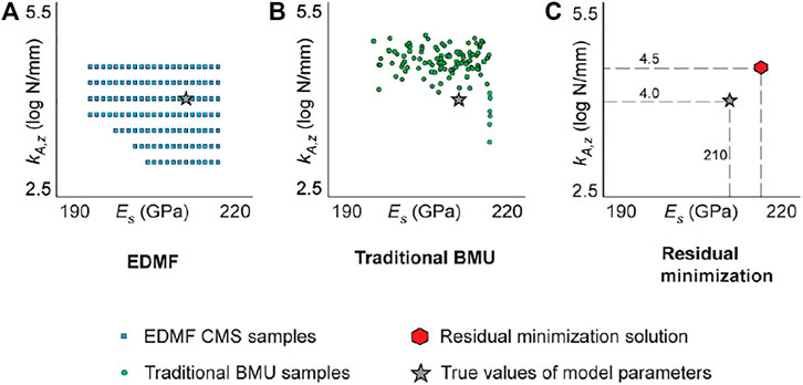
FIGURE 1. Comparison of data-interpretation solutions obtained using (A) EDMF, (B) traditional BMU, and (C) residual minimization for the Ponneri Bridge case study. The results are adapted from the Ponneri Bridge case study described in Pai (2019). EDMF and modified BMU provide accurate, albeit less precise, solutions compared with traditional BMU, and residual minimization.
EDMF has been shown analytically and empirically to be equivalent to BMU when a box-car shaped likelihood function is used for incorporating information from measurements (Reuland et al., 2017; Pai et al., 2018, 2019). This likelihood function is determined using the same EDMF thresholds. As these thresholds are calculated based on explicit quantification of bias, the function is robust to incomplete knowledge of correlations, as is EDMF. Therefore, BMU with a modified likelihood function, similar to EDMF, provides more accurate solutions compared with traditional BMU and RM. EDMF may be interpreted as a practical implementation of BMU with uniform uncertainty characterization for model-based data interpretation.
Challenges in Sensor Data Interpretation
Use of sensor data for updating knowledge of structural behavior enhances asset management. However, many challenges exist related to development of measurement systems, data processing and development of appropriate physics-based models. Most data-interpretation studies have been limited to laboratory experiments and simulated hypothetical cases. Extending conclusions to full-scale cases must be done with care. In this section, a few common challenges are discussed along with methods to overcome weaknesses.
Outliers in Data
Use of data interpretation methodologies typically involves the assumption that measurement datasets do not include spurious data. Outliers are anomalous measurements that may occur due to sensor malfunction (Beckman and Cook 1983) and other factors such as environmental and operation variability (Hawkins 1980). The presence of outliers in measurement datasets reduces accuracy and performance of structural identification methods (Worden et al., 2000; Pyayt et al., 2014; Reynders et al., 2014).
Most developments related to outlier detection are focused on continuous monitoring applications (Burke 2001; Hodge and Austin 2004; Ben-Gal 2006; Posenato et al., 2010; Vasta et al., 2017; Deng et al., 2019). These methods are not suitable to detect outliers in datasets that consist of sparse measurements recorded during static load tests (Pasquier et al., 2016). Suggested an outlier-detection method for EDMF based on sensitivity of identified solutions to each measurement. A measurement data point that falsifies uncharacteristically high number of models was flagged as a potential outlier. A drawback of this approach is that when one measurement data point is much more informative than other measurement data points, this data point could be labelled as an outlier even when the measurement is valid. Exclusion of the most informative data point from identification procedures may severely limit the information gained from monitoring.
Proverbio et al. (2018a) suggested comparing the expected performance of a sensor configuration (as estimated with a sensor placement algorithm) with observed performance based on monitoring data. Measurement data that showed large variations from expected performance were flagged as outliers and excluded during identification. This approach is able to detect outliers in sparse datasets and overcomes several limitations of other outlier-detection methodologies (Proverbio et al., 2018a).
Measurement System Design
The use of information entropy for measurement system design has been studied extensively (Papadimitriou et al., 2000; Papadimitriou 2004; Robert-Nicoud et al., 2005b; Kripakaran and Smith 2009). However, most researchers have not accounted for the possibility of mutual information between sensor locations while designing measurement systems (Papadimitriou and Lombaert 2012; Barthorpe and Worden 2020). Papadopoulou et al. (2014) developed a hierarchical sensor-placement algorithm that accounts for mutual information. This algorithm was demonstrated for designing a measurement system to study wind around buildings (Papadopoulou et al., 2015, 2016). Bertola et al. (2017) extended this algorithm for multi-type sensor placement to monitor civil infrastructure systems under several static load tests.
Typically, measurement data for structural identification is acquired by conducting either dynamic or static load tests. Information from dynamic and static load tests may be either unique or redundant (Schlune et al., 2009). Many studies have been carried out to maximize information gained through dynamic and static load tests (Goulet and Smith 2012; Argyris et al., 2017). However, little research has been carried out for design of measurement systems involving static and dynamic load tests. Bertola and Smith (2019) suggested an information entropy-based methodology for designing measurement systems when dynamic and static load tests are planned.
There are several challenges involved with designing measurement systems. The task of sensor placement is computationally expensive and requires use of adaptive search techniques such as global (Chow et al., 2011) and greedy (Kammer 1991; Bertola and Smith 2018) searches. Also, since measurement-system design methodologies cannot be easily validated, Bertola et al. (2020a) developed a validation strategy using hypothesis testing. Then, the optimal measurement-system design depends on several performance criteria such as information gain, monitoring costs and robustness of information gain to sensor failure. Bertola et al. (2019) introduced a framework where measurement-system recommendations are made based on a multi-criteria decision analysis that accounts for several performance-criterion evaluations as well as asset-manager preferences.
The task of measurement system design is critical to ensure that measurement data for structural identification is informative and leads to reduction in uncertainty related to system behavior (Peng et al., 2021a). Poor design of measurement systems will lead to weak justification for monitoring and ultimately, to uninformed asset-management decision making. Measurement systems must thus be justified using cost-benefit analyses. Bertola et al. (2020b) proposed a framework to evaluate the value-of-information of measurement systems based on the influence of the information collected on the bridge reserve-capacity estimation.
Measurement-system-design methodologies has the potential to select informative data among large existing data sets. Wang et al. (2021) proposed an entropy-based methodology to reduce the number of measurements used for data interpretation. Using the reduced sets of data (up to 95% reduction) led to additional information gain compared with using complete data sets.
Model-Class Selection
Physics-based models include parameters that represent physical phenomena affecting structural behavior. For real-world applications, not all phenomena affecting infrastructure behavior are known. Engineering knowledge is important for development of physics-based models and inclusion of appropriate parameters.
As structural behavior is not known perfectly, some parameters of physics-based models are quantified as random variables. As previously described, appropriate quantification of their values is necessary for accurate data interpretation. The task of model-based data interpretation is to reduce uncertainty related to parameter values that govern structural behavior.
Model-based data interpretation involves searching for solutions (parameters that lead to model behavior that is compatible with measurements) in a large model-parameter space. The larger the parameter space to be explored, the greater the computational cost of finding solutions. Moreover, all measurements are not informative for all parameters. Hence, selecting parameters that are compatible with the information that is available from measurements is important to improve computational efficiency while maintaining precision.
For a given physics-based model, from a large set of potential model parameters, many smaller subsets of parameters can be selected for identification. Each of these subsets defines a model class for identification. The task of selecting an appropriate model class for identification and subsequent predictions of structural behavior is called model-class selection (or feature selection) (Liu and Motoda 1998; Bennani and Cakmakov 2002; Guyon and Elisseeff 2006).
Selection of a model-class for identification without utilizing information from measurements is called as a-priori model class selection. Traditionally, selection of a model-class has been carried out using sensitivity analysis based on linear-regression models (Friedman 1991). Other methods include assessment of coefficient of variation, analysis of variance (Van Buren et al., 2013; Van Buren et al., 2015), information criterion such as Akaike information criterion (Akaike 1974) and Bayesian information criterion (Schwarz, 1978) and regularization.
Most methods available in literature are restricted to linear models and Gaussian uncertainties. Also, these methods focus on finding a good subset of parameters that influence model response at one measurement location. For civil infrastructure, model response at various measurement locations may not be governed by the same set of parameters. To select an optimal model class that is suitable for all measurement locations, either the importance of parameters to model responses have been averaged (Matos et al., 2016) or an intersection of parameters important to response at all sensor locations (Van Buren et al., 2015) have been assumed. However, novel sensor placement strategies (Papadopoulou et al., 2015; Argyris et al., 2017; Bertola et al., 2017) have been developed that minimize number of sensors and maximize information from each sensor. Ideally, these strategies result in each sensor providing new information about model parameters. Under such conditions, use of averaged sensitivities is not an appropriate metric for model-class selection.
Pai et al. (2021) proposed a novel model-class selection method to overcome many challenges related to existing methods, especially in context of developments related to novel sensor placement strategies. In this method, the selection of parameters is not carried out by evaluating the importance of parameters to response at each measurement location. Instead, a global understanding of structural behavior is evaluated using clustering. As parameter values vary, global changes in structural behavior are estimated using clustering. Parameters governing these clusters of response are identified using a classifier whose features are selected based on a greedy search.
Validation
EDMF, when compared with traditional BMU and RM, has been shown to provide accurate model updating for theoretical cases using simulated measurements (Goulet and Smith 2013; Pasquier and Smith 2015; Reuland et al., 2017). In these theoretical comparisons, the ground-truth values are known. For assessment of accuracy of full-scale structures, cross-validation methods have the potential to demonstrate quantitative validation.
Comparisons of EDMF with traditional BMU and RM have been made for full-scale case studies using leave-one-out cross-validation (Pai et al., 2019) and hold-out cross-validation (Pai et al., 2018). In these comparisons, one or more measurements (data points) are excluded during identification. Subsequent to identification, the updated parameter values are used to predict response at measurement locations that were excluded. If the predicted response is similar to the measurement value, then structural identification is assumed to be validated (Vernay et al., 2018).
However, in cross-validation methods (Golub et al., 1979; Kohavi, 1995) such as leave-one-out and hold-out cross-validation (Hong and Wan 2011), the data points left out may or may not contain new information. If information contained in the validation dataset is not exclusive, then validation with redundant data is not suitable for assessment of accuracy. Therefore, information entropy metrics (Papadopoulou et al., 2015; Bertola and Smith 2019) may be used to assess exclusivity of information in validation data and suitability of validated solutions for making further predictions to support asset management decision-making.
Pai and Smith (2021) demonstrated the utility of assessing mutual information between data used for identification and validation to ensure appropriate assessment of accuracy. Structural identification of a steel-concrete composite bridge was carried out using the three data-interpretation methodologies described in Methodologies for Model-Based Sensor Data Interpretation. To assess accuracy of the identification results, leave-one-out and hold-out cross-validation strategies were carried out. As validation data became more exclusively informative (less mutual information with identification data), the number of cases where identification was assessed to be accurate was observed to reduce. Therefore, using exclusive information (not redundant information) for validation may lead to better assessment of accuracy of structural identification.
Case Studies
Model-based data interpretation enables use of updated knowledge of structural behavior for prognosis and estimation of capacity available beyond design calculations. The use of a physics-based model enables propagation of uncertainty from various sources during prognosis to support the extrapolation that is needed for asset management decision-making. These decisions may be related to remaining fatigue life estimation, retrofit design, load-carrying capacity, post-earthquake capacity, localization of damage and ultimately, replacement.
Challenges in Sensor Data Interpretation outlines key challenges in practical implementation of the three data-interpretation methodologies that are described in Methodologies for Model-Based Sensor Data Interpretation. Laboratory experiments are designed to reduce unknowns and uncertainties cannot contribute to challenges that are typically encountered in real world-applications. In this section, a summary of case studies that have been evaluated from 2015 to 2020 are described. A list of these case studies is provided in Table 1 with a brief description.
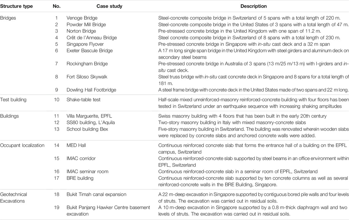
TABLE 1. Full-scale case studies evaluated with monitoring data since 2015. Case studies evaluated before 2015 are described in Smith (2016).
Reserve Capacity Estimation
Some of the case studies listed in Table 1 have been studied to improve understanding of reserve capacity in built infrastructure. Reserve capacity is defined as the capacity available in built infrastructure beyond code-specified requirements related to the critical limit state (Proverbio et al., 2018c). Typical limit states are defined to be either fatigue failure, or serviceability limits. For the ultimate limit state, a special strategy has been developed (Proverbio et al., 2018c). Quantifying reserve capacity provides useful information for performing asset-management tasks such as comparing repair scenarios with replacement. Case studies listed in Table 2 have been investigated to identify reserve capacity related to the ultimate limit state (ULS), the serviceability limit state (SLS) and fatigue.
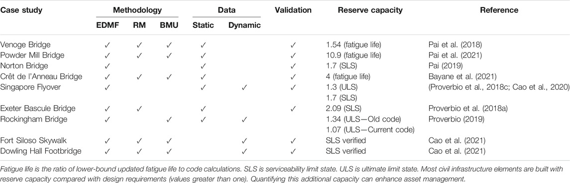
TABLE 2. Methodologies compared and reserve capacity assessments of civil infrastructure cases according to the critical limit state in parentheses and determined using EDMF.
In Table 2, the data-interpretation methodology used to interpret monitoring data (static and dynamic) is indicated. Typically, data is interpreted using multiple methodologies and solutions obtained are compared and validated using methods described in Validation. Only solutions that have been validated are used to predict the reserve capacity. References that provide more details regarding these evaluations have been provided in the table. The reserve capacities are calculated so that unity is the situation where calculations with all relevant safety factors exactly attains the critical limit state. A reserve capacity that is greater than unity indicates that there is additional safety built into the structure beyond the critical limit state.
Reserve capacities listed in Table 2 suggest that most built infrastructure has significant reserve capacity compared with code-based requirements, and this confirms similar observations made previously (Smith 2016). Quantifying this reserve capacity using monitoring data enhances decision making related to asset-management actions. Overdesign reflected by reserve capacity values that are over one also leads to unnecessary material and construction costs as well as unnecessarily high carbon footprints.
For two case studies listed in Table 2, Singapore Flyover and Rockingham Bridge, the reserve capacity assessment was compared with the present verification code (CEN 2012a; b; NAASRA 2017) and the design code at the time of construction (NAASRA 1970; BSI 1978, 1984). Both infrastructure elements were significantly over-designed during construction with respect to the prevalent codes at the design stage. Additionally, for the Singapore Flyover, not only did the reserve capacity change, the critical limit state at design stage was different from the new-code-verification stage (Proverbio et al., 2018c). Monitoring and reserve-capacity assessment with enhanced models can potentially avoid unnecessary repair actions in such situations.
For most of the case studies listed in Table 2, EDMF was able to provide accurate data interpretation upon validation to support asset management. This observation was made for various types of bridges, from different decades, built with a range of materials and monitored to provide heterogeneous data, including static and dynamic data. Validation was possible because of the explicit quantification of multi-sourced biased uncertainties as well as the intrinsic robustness of EDMF to unknown correlations as described in Error-Domain Model Falsification.
Other Applications
Interpreting monitoring data with physics-based models can also be used to enhance decision making in other application areas. For example, applications in post-earthquake hazard assessment, risk mitigation during excavations, damage detection and occupant localization have been studied.
Post-earthquake monitoring data has been used to update physics-based models and predict residual capacity (Reuland et al., 2019a). Residual capacity is defined as the ability of an infrastructure to resist aftershocks and subsequent earthquake events. While EDMF has been used for post-earthquake evaluation of many case studies (Reuland 2018; Reuland et al., 2015, 2017), due to limitations in data available from real earthquakes, validation with data from aftershocks could not be performed for every case study. However, data-interpretation results from the shake table test were validated to show that EDMF provided the accurate identification (Reuland et al., 2019b). Models updated with measurement data reduce uncertainty in predictions and improve understanding of structural capacity. This enhanced knowledge can be used to avoid unnecessary post-hazard closures of buildings while supporting a risk-based assessment to either close or retrofit essential buildings.
Wang et al. (2020, 2019) studied the use of data-interpretation methodologies for reducing uncertainty related to excavations. Data from one stage of excavation is used to predict behavior at further stages of excavation leading to less conservative practices. In addition, Wang et al. (2021) combined EDMF and a hierarchical algorithm based on a joint-entropy objective function to select field response measurements that provide the most useful knowledge of material parameter values in a model-based data interpretation exercise. Also, (Cao et al., 2019a), combined information from monitoring data and physics-based models to predict damage location in train wheels to improve infrastructure management.
Another application of monitoring data is localizing occupants within buildings. Information about occupancy in buildings can be used for security needs and non-intrusive monitoring in care-homes and other applications. Drira et al. (2019) investigated the use of model updating to localize occupants in buildings. These investigations were performed on floor slabs of buildings with various structural and occupancy characteristics. EDMF was found to be able to accurately localize and track occupants in buildings with floor-vibration data from sparse sensor configurations.
In this section, applications of data-interpretation to real-world case studies are briefly presented. More information regarding these studies can be found in the references provided in Tables 2, 3. Challenges encountered while evaluating these case studies along with relevant research are presented briefly in Challenges in Sensor Data Interpretation.
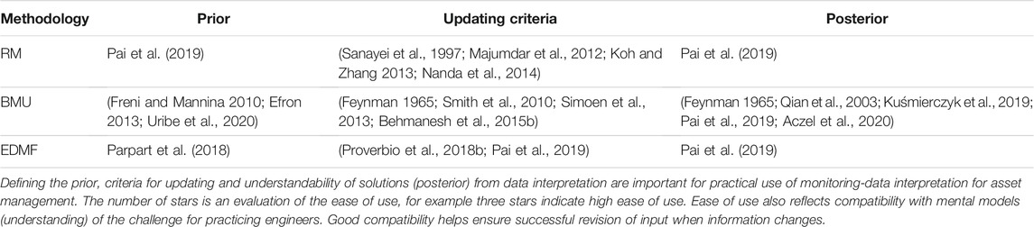
TABLE 3. Comparison of ease of use of model-based data interpretation methodologies at three stages of application.
In the next section, methodology maps have been developed following experience with the case studies presented in this section. Significant literature was also reviewed while evaluating these case studies and knowledge acquired from these reviews was also used to develop these maps. While the maps are in no way absolute indications of the best method for all cases, they are intended to guide users towards appropriate choices of methodologies to interpret data.
Methodology Maps
In this section, methodology maps are presented that guide the choice of the best data interpretation methodology based on the following four criteria:
• Magnitude of uncertainty
• Magnitude of bias
• Model complexity
• Ease of implementation in practice
The magnitude of uncertainty refers to the total uncertainty (difference between model and measured response) affecting the task of data interpretation at each measurement location. This includes combination of uncertainties from sources such as sensor noise, operational conditions, modelling assumptions, parametric uncertainty, geometrical simplifications and numerical errors. For example, if the combined uncertainty is assumed to be zero-mean Gaussian then the magnitude of uncertainty is defined by the standard deviation of the distribution. If the combined uncertainty is assumed to be uniformly distributed, then the magnitude of uncertainty is defined by the range of the distribution (upper bound minus the lower bound value).
The magnitude of bias refers to the systematic bias between model response and real system behavior. As most civil engineering models are safe for design, implicit assumptions made during model development are biased to provide conservative predictions of system behavior. For example, if the combined uncertainty is assumed to be Gaussian, then the magnitude of bias is defined by the non-zero mean of the distribution. If the combined uncertainty is defined as a uniform distribution then the bias magnitude is defined as the mid-point of the uniform distribution (0.5 times range of the distribution plus the lower bound value).
Model complexity refers to the level of model detail and fidelity of the model to real system behavior. For example, a three-dimensional FE model of a bridge is more complex than an analytical one-dimensional model based on Euler-Bernoulli beam theory. The computational cost associated with obtaining solutions for the task of structural identification is often related to the model complexity. A complex model is computationally more expensive than a simpler model. Complex models (for example FE models) are often defined by more parameters than simple models (for example a Euler-Bernoulli beam) that may have to be identified, which would increase number of simulations required, thereby increasing the computational cost. However, a complex model could have better fidelity with real system behavior compared with a simpler model.
Three methodology maps are developed with magnitude of uncertainty and systematic bias as the two axis. These methodology maps correspond to three levels of model complexity: low (Low Model Complexity), medium (Medium Model Complexity) and high (High Model Complexity). Maps in these sections are two-dimensional projections of a three-dimensional map, which is schematically shown in Figure 2. This three-dimensional map is separated into three maps along the axis of model complexity. For the purpose of developing methodology maps in this paper, the discrimination between low, medium and high model complexity, uncertainty and bias are quantified based on the experience of authors gained by evaluating many case studies as described in 4. Using the Methodology Maps includes examples on the use of these methodology maps to select an appropriate data-interpretation methodology.
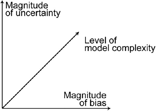
FIGURE 2. Schematic representation of the three dimensions of a methodology map to guide practitioners in selecting the appropriate data-interpretation methodology.
Other than the three criteria of the magnitude of uncertainty, systematic bias, and model complexity, another criterion, ease of implementation, governs the choice of data interpretation methodologies. Ease of implementation in practice refers to the challenges associated with the data interpretation task. This includes computational costs, prior knowledge, developing the strategy for updating (for example the likelihood function, see Traditional Bayesian Model Updating) and understanding solutions of the interpretation task. Typically, this criterion governs whether data-interpretation can be applied in practical contexts.
In the next sections, methodology maps that support users in selecting appropriate methodologies based on these criteria are presented. The data interpretation methodologies that are considered are RM (see Residual Minimization), BMU (see Traditional Bayesian Model Updating and Bayesian Model Updating With Parameterized Model-Error) and EDMF (see Error-Domain Model Falsification). The objective of these maps is to help users select a good data-interpretation methodology according to criteria related to uncertainty (amount as well as bias), model complexity and transparency (ease-of-use).
Low Model Complexity
A methodology map to select an appropriate data interpretation methodology considering magnitude of uncertainty and magnitude of systematic bias for interpretation using models with low complexity (computational cost) is presented in Figure 3. Low complexity models are analytical models such as beam deflection equations and simple 1D beam models. Therefore, models that have a complexity O(n) and finite element models with a small number of nodes and elements (such as beam element models with O(n3) complexity) can be considered as low complexity models, where n is number of degrees of freedom.
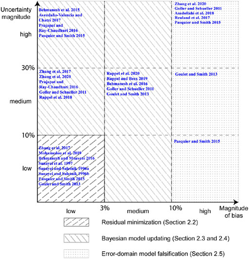
FIGURE 3. Methodology map describing best use of data-interpretation methodologies in relation to systematic bias and magnitude of uncertainty when using models with low complexity (computational cost).
The two axes of the map shown in Figure 3 are uncertainty magnitude and bias in uncertainty. In civil engineering contexts, the main contribution for this uncertainty involves model error, which is the difference between response obtained using a physics-based model and real system behavior (not known). For the purpose of developing methodology maps in this paper, the discrimination between low, medium and high uncertainty as bias as shown in Figure 3 is quantified based on the experience of authors in evaluating many case studies as described in 4.
RM (or calibration), as shown in Figure 3, is suitable for tasks involving low bias (less than 3% bias from zero mean) and low uncertainty magnitudes (less than 10%). Such conditions require models that are high-fidelity approximations of reality, which is not common in full-scale civil engineering evaluations. However, RM is also suitable for developing regression models and data-only approaches (Bogoevska et al., 2017; Hoi et al., 2009; Laory et al., 2013; Neves et al., 2017; Posenato et al., 2008, 2010). Calibration in this context is typically limited to estimating coefficients of regression models where interpolation predictions are required.
BMU, involving either traditional or more advanced applications, is suitable for tasks that have low to medium bias (up to 10% deviation from zero-mean) and low to high uncertainty magnitudes. Traditional implementation of BMU is suitable for tasks with low model bias. This encompasses tasks that may be performed using RM such as Bayesian optimization of data-only models (Gardoni et al., 2002). BMU is best employed for analyzing laboratory experiments conducted in controlled environments (Prajapat and Ray-Chaudhuri 2016; Zhang et al., 2017; Rappel et al., 2018, 2020; Mohamedou et al., 2019; Rappel and Beex 2019) to reduce bias from modelling assumptions. BMU is also appropriate for analyzing large-scale systems when the physics-based models developed are unbiased approximations of reality as is often the case for mechanical-engineering applications (Abdallah et al., 2017; Avendaño-Valencia and Chatzi 2017; Hara et al., 2017; Argyris et al., 2020; Cooper et al., 2020; Patsialis et al., 2020).
When the bias is neither low nor high (between 3 and 10% deviation from zero-mean), advanced BMU methods can be used for data-interpretation. These include parameterization of the model error terms (Kennedy and O’Hagan 2001) as explained in Bayesian Model Updating With Parameterized Model-Error. Users have to be careful while employing these advanced methods as they may provide more precise solutions than EDMF (Goulet and Smith 2013; Pasquier and Smith 2015), while also being prone to unidentifiability challenges (Prajapat and Ray-Chaudhuri 2016; Song et al., 2020) due to requirements of estimating many parameters relative to information available from measurements.
While RM is the best method when uncertainty and bias magnitudes are low, EDMF is suitable (not necessarily optimal) for all tasks ranging from low to high uncertainty magnitudes and bias. However, EDMF was developed specifically for analyzing tasks with high magnitude of bias such as civil infrastructure (Goulet and Smith 2013). Models of civil infrastructure typically involve conservative modelling assumptions that lead to large systematic biases between model and real behavior (Goulet et al., 2013). Application of EDMF to tasks with large magnitude of bias and uncertainty have been listed in Table 2.
Validation of solutions obtained with data-interpretation is important as explained in Validation. Many researchers have used data-interpretation methodologies under conditions where the inherent assumptions are not satisfied in reality. RM does not account for model bias in the traditional form as described in Residual Minimization. However, applications of RM to tasks with large uncertainty magnitudes and large bias are common in literature (Chen et al., 2014; Sanayei et al., 2011; Sanayei and Rohela 2014). Similarly, traditional BMU has also been applied to tasks involving large systematic bias (Behmanesh et al., 2015a; b). While solutions obtained in such applications may be suitable for damage detection (interpolation) (Li et al., 2016), they are not suitable for asset management tasks where extrapolation predictions are required (Brynjarsdóttir and O’Hagan, 2014; Song et al., 2020).
Low model complexity ensures that not only deterministic RM but also probabilistic BMU and EDMF may be used to interpret data. Increasing model complexity increases the computational cost associated with practically implementing probabilistic data-interpretation methodologies such as BMU and EDMF.
Medium Model Complexity
In this section, a methodology map to select an appropriate data interpretation methodology while using medium complexity models is presented. Figure 4 presents a methodology map to select the most appropriate data interpretation methodology based on the criteria of systematic bias and model uncertainty when the complexity of models available to interpret data is medium. Medium complexity models include finite element models involving two and three-dimensional elements such as shell and brick elements. These models when used for static and modal analysis involving matrix inversion have a complexity of O(n3), where n is the number of degrees of freedom in the model.
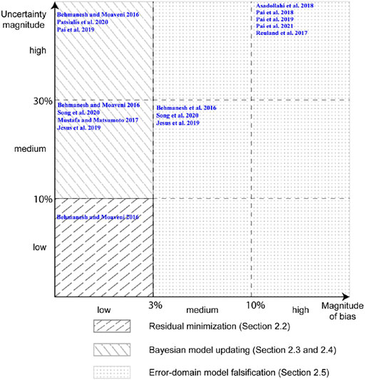
FIGURE 4. Methodology map describing best use of data-interpretation methodologies in relation to systematic bias and magnitude of uncertainty when using models with medium complexity (computational cost).
RM, as described in Residual Minimization, is suitable for tasks with low systematic bias and low magnitude of uncertainty using models with medium complexity (Behmanesh and Moaveni 2016). While medium complexity models are computationally more expensive than low complexity models, efficient application of RM for model updating is possible using adaptive sampling methods (Bianconi et al., 2020).
BMU in its traditional forms may be used for tasks with low levels of systematic bias and low-to-high uncertainty magnitudes. However, use of medium-complexity models for probabilistic evaluation is challenging. Adaptive sampling methods such as Markov Chain Monte Carlo (MCMC) sampling (Qian et al., 2003), transitional MCMC (Ching and Chen 2007; Betz et al., 2016) and Gibbs sampling (Huang and Beck 2018) may help to reduce the computational cost. However, the increase in number of parameters to be identified (in addition to the model parameters) while using the advanced forms of BMU (Kennedy and O’Hagan 2001; Behmanesh et al., 2015a) may be prohibitive for practical data interpretation using medium complexity models. Additionally, complex sampling and interpretation methods increase difficulty of practical implementation, which will be discussed in Suitability for use in Practice.
EDMF is suitable for all levels of systematic bias and uncertainty magnitudes, particularly cases involving high systematic bias (Reuland et al., 2017; Proverbio et al., 2018b; Pai et al., 2018, 2019, 2021; Reuland et al., 2019a; Reuland et al., 2019b; Drira et al., 2019; Wang et al., 2020). Depending upon the computational constraints, EDMF can be implemented with either a grid sampling approach or an adaptive sampling (Raphael and Smith 2003; Proverbio et al., 2018b). Although grid sampling is computationally expensive, it is convenient when data interpretation has to be revised with new information (Pai et al., 2019). For tasks involving medium levels of systematic bias, BMU may be used with its advanced forms. However, using these implementations with medium complexity models may be inefficient. EDMF is suitable for interpreting tasks with medium levels of systematic bias and provides choices for implementation of adaptive and grid-based sampling approaches to reduce computational cost while interpreting with models of medium complexity.
High Model Complexity
In this section, a methodology map to select an appropriate data interpretation methodology while using high complexity models is presented. In Figure 5, a methodology map is presented to select the most appropriate data interpretation methodology based on the criteria of systematic bias and model uncertainty when the complexity of models available to interpret data is high. Models such as finite element models that incorporate complex physics such as material non-linearity, geometric non-linearity as well as analysis involving contact mechanics and transient analysis can be considered as high complexity models. These models have many degrees of freedom and involve iterations either over time domain (transient analysis) or for convergence related to non-linear simulations. Each of these iterations with a model of complexity O(n3) leads to high computational cost.
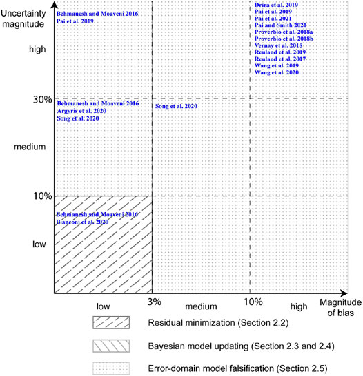
FIGURE 5. Methodology map describing best use of data-interpretation methodologies in relation to systematic bias and magnitude of uncertainty when using models with high complexity (computational cost).
RM, as described in Residual Minimization, is suitable for tasks with low magnitudes of uncertainty and systematic bias. However, as previously mentioned, this is a popular methodology in practice (Bogoevska et al., 2017; Hoi et al., 2009; Laory et al., 2013; Neves et al., 2017; Posenato et al., 2008, 2010) due to its ease of implementation and its low computations cost. The computational cost of using RM with high complexity models is usually much lower than other probabilistic methodologies. Strategies such as particle swarm optimization (Gökdaǧ and Yildiz, 2012), genetic algorithms (Chou and Ghaboussi 2001; Gökdaǧ, 2013) and other sampling methods (Zhang et al., 2010; Majumdar et al., 2012) have been used by researchers to make RM over many dimensions a cost-effective data interpretation methodology.
While BMU may be used for data-interpretation tasks involving medium-to-high systematic bias and uncertainties, the cost of using high complexity models is prohibitive. Therefore, EDMF is a better choice for interpretation tasks involving medium-to-high systematic bias (greater than 3%) and uncertainties (greater than 10%) using high complexity models. EDMF, similar to BMU, is suitable for medium-to-high magnitudes of uncertainty with models of all levels of complexity and can be implemented with grid sampling approach and adaptive sampling (Raphael and Smith 2003; Proverbio et al., 2018b). EDMF has the added advantage of being computationally efficient when data interpretation has to be revised compared with BMU (Pai et al., 2019). The task of data interpretation in practice is typically iterative in nature due to changing operational and environmental conditions and also, as new information becomes available (Pasquier and Smith 2016; Reuland et al., 2019b; Pai et al., 2019).
Scalability of RM to various levels of model complexity and the array of sampling methodologies available for BMU demonstrate that significant research effort has been directed at improving computational efficiency. While this is sufficient for individual analyses at a given moment, such as damage detection, the task of asset management and prognosis is iterative in nature due to changing conditions and emergence of new information. Non-adaptive sampling methods and heuristic searches (Sanayei et al., 1997) are more amenable for use in practice for repeated data interpretation compared with sampling methods that would require a complete restart (Pai et al., 2019). RM and EDMF are most suitable for use of non-adaptive sampling methods making them better choices when using high-complexity models.
Suitability for use in Practice
Methodology maps presented in Figures 3–5 assist a user in selecting an appropriate data interpretation methodology considering uncertainty magnitudes, bias magnitudes and model complexity. However, practical implementation of these methodologies presents additional challenges. Application of any data interpretation methodology has three components:
• Estimation of prior distribution of model parameters.
• Updating strategy (objective function for RM, likelihood function for BMU and falsification thresholds for EDMF) as well as solution-exploration methods (for example, optimization techniques, adaptive sampling etc.).
• Interpretability of posterior (updated) distribution of model parameters for decision making.
The above three components are in addition to the task of data collection and quality control checks, such as assessing sensor noise and detection of outliers, that have to be performed.
The BMU methodology has gained popularity in the research community with an objective to support real-world data-interpretation tasks. Therefore, applicability of BMU is discussed first in this section. Subsequently, applicability of RM and EDMF is discussed relative to challenges in practical implement of BMU.
The choice of prior distribution for BMU is one of the first steps (see Traditional Bayesian Model Updating). Appropriate quantification of prior distributions of parameters in a model class can significantly influence results obtained with BMU (Freni and Mannina 2010; Efron 2013; Uribe et al., 2020). In the context of civil infrastructure, model parameters related to aspects such as boundary conditions are specific to each case and cannot be generalized. This complicates the task of informatively quantifying the prior of model parameters.
Traditional BMU, as described in Traditional Bayesian Model Updating, does not include parameters related to the model error in the model class. Novel BMU developments such as hierarchical BMU (Behmanesh et al., 2015b) estimate errors to improve accuracy, as explained in Bayesian Model Updating With Parameterized Model-Error. However, a small number of studies allow for various sources of uncertainty for specific measurement locations. Simoen et al. (2013) studied the effect of correlations on the posterior of model parameters, albeit with same error variance for all data points. Explicit modelling of the prediction error (variance, bias, and correlations) for specific measurement locations increases dimensionality of the inverse task. Consequently, this may lead to identifiability challenges and high computational costs (Prajapat and Ray-Chaudhuri 2016).
Another implementation step involved in carrying out BMU is the development of the likelihood function that incorporates information from measurements. Traditionally, this is defined by a zero-mean independent Gaussian PDF as shown in Eq. 2. Many researchers have demonstrated that the use of a zero-mean independent Gaussian likelihood function provides inaccurate solutions in the context of civil infrastructure (Simoen et al., 2012; Goulet and Smith 2013; Pasquier and Smith 2015). The choice of the likelihood function and its developments affect the accuracy of model-parameter estimation in BMU (Smith et al., 2010). Aczel et al. (Aczel et al., 2020) emphasized the need to perform checks for robustness to this choice while selecting a likelihood function (and priors). Appropriateness of choices made in estimating priors and developing the likelihood function can only be measured by testing predictions against reality (Feynman 1965), which in the absence of situations of either simple theoretical or experimental cases, requires statistical knowledge.
The results obtained with BMU are a joint posterior PDF of model parameters. Interpretation of this PDF is important for making decisions based on updated knowledge acquired from measurements. However, for appropriate decision making, asset managers have to be provided with information of the joint posterior PDF along with assumptions and choices that were made to define it, such as the prior, likelihood function and the physics-based model. Additionally, statistical knowledge is necessary for interpreting the posterior PDF (Aczel et al., 2020).
Application of BMU also suffers due to the requirement of adaptive samplers such as Markov Chain Monte Carlo sampling (Tanner 2012) and other variants (Ching and Chen 2007; Angelikopoulos et al., 2015; Huang and Beck 2018), which are difficult to implement (Pai et al., 2019). Random sampling such as Monte Carlo sampling may lead to poor and inaccurate estimation of the posterior (Qian et al., 2003) leading to inappropriate and unsafe asset management (Kuśmierczyk et al., 2019).
RM is widely used in practice despite providing inaccurate solutions in presence of large magnitudes of uncertainty and systematic bias as detailed in Residual Minimization, Low Model Complexity, Medium Model Complexity, High Model Complexity. This is due to the simplicity in application of RM. In RM, there is no strong requirement regarding the estimation of priors for model parameters. In typical civil-engineering contexts, a uniform prior is assumed for RM. The updating criteria is a minimization of error between model response and measurements. This minimization task may be performed using optimization algorithms (Majumdar et al., 2012; Koh and Zhang 2013; Nanda et al., 2014) as well as simple trial and error methods (Sanayei et al., 1997). Finally, the solution is a unique set of model-parameter values that provide the least error between model response and measurements. Admittedly, uniqueness of the result reduces the possibility of error in interpretation of solution due to lack of statistical knowledge.
EDMF, in a similar way to RM, has advantages over BMU due to ease of implementation. Additionally, EDMF may be used for a wider range of applications with large magnitudes of uncertainty and bias, as explained in Low Model Complexity, Medium Model Complexity, High Model Complexity. In EDMF, the prior PDF of model parameters is estimated using engineering knowledge and is typically assumed to be uniform. This is compatible with observations by researchers that using heuristic information can lead to quantification of appropriate priors (Parpart et al., 2018).
The updating procedure in EDMF is based on the philosophy of falsification as hypothesized by Karl Popper (Popper 1959). In EDMF, model instances that provide responses that are incompatible with measurements are rejected (falsified). The criteria for compatibility are defined based on the uncertainty associated with the interpretation task from sources such as modelling imperfections and sensor noise. As the engineer has to quantify this uncertainty and determine the falsification criteria, basic knowledge of statistical bounds is required. Fortunately, practicing engineers often use bounds to describe uncertainty.
The solution obtained with EDMF is a population of model instances that are compatible with observations. Due to lack of complete knowledge of uncertainties, all model instances in this solution set are assumed to be equally likely. The asset manager may use this population to make decisions. Unlike RM, the asset manager, while using EDMF, has to either use the entire population of solutions for decision making or may use specific model instances for decision making based on expert opinion and statistical knowledge. Working with a population of solutions rather than a joint posterior PDF (as obtained with BMU) requires less statistical knowledge and is more transparent for use by decision makers.
Application of EDMF is typically carried out with grid sampling (Pai et al., 2019), which has practical advantages over adaptive sampling methods (Proverbio et al., 2018b) when information has to be interpreted iteratively. Other sampling methods, such as Monte Carlo sampling and Latin hypercube sampling, have also been used to perform EDMF (Cao et al., 2019b). Unlike BMU, EDMF does not require sampling from the posterior to achieve accuracy, which allows use of simpler sampling techniques.
RM is the easiest method for use in practice, albeit with a limited range of applications as described in Residual Minimization, Low Model Complexity, Medium Model Complexity, High Model Complexity. BMU has a wider range of applications based on uncertainty considerations but is limited by challenges for use in practice due to expertise required in implementation. EDMF may be employed for a wide range of applications and overcomes many practical limitations associated with BMU for probabilistic data-interpretation. A summary of this discussion is presented schematically in Table 3.
In Table 3, the checkmarks indicate ease of implementation related to the specific step involved such as estimating the prior. The number of checkmarks from one to three indicate increasing ease of implementation. EDMF and RM have greater ease of implementation compared with BMU while performing the steps involved such as estimating the prior, updating, sampling and interpreting the posterior (solutions). EDMF, with possibilities for a wider range of applications as explained in Residual Minimization, Low Model Complexity, Medium Model Complexity, High Model Complexity, and relatively simpler implementation should thus be the methodology of choice for interpreting data related to most civil-infrastructure assessment tasks.
To aid in application of EDMF to full-scale case studies, an open access software called MeDIUM (Measurement Data Interpretation Using Models) has been developed. The software is available for downloading at the following link: https://github.com/MeDIUM-FCL/MeDIUM. MeDIUM facilitates predictions (prognoses), particularly extrapolations, through representing ranges of values of variables. MeDIUM is a software implementation of EDMF with additional tools for validation and assessment of uncertainty estimations. MeDIUM improves accessibility of EDMF to new users of data interpretation methods especially for the context of data interpretation when managing civil infrastructure. With this software, users may interpret monitoring data to obtain validated and updated distributions of model parameters to support asset management decision making. The welcome tab of the software is shown in Figure 6.
FIGURE 6. A software for measurement data interpretation using uncertain models (MeDIUM) for effective and sustainable asset management.
The software provides users functionalities such as performing what-if analysis. Users may assess the impact of uncertainty estimation on solutions of EDMF with simple sliders that controls factors such as magnitude of uncertainty and target reliability of identification. Users are also provided with options to perform cross-validation of solutions by leaving out (holdout) measurements. The users have full control over the measurements to be left out and uncertainty definitions. The results of performing EDMF and validation may also be visualized with the software.
Using the Methodology Maps
Methodology maps presented in Low Model Complexity, Medium Model Complexity, High Model Complexity, have been developed with knowledge of the data-interpretation methodologies that are described in Residual Minimization, Traditional Bayesian Model Updating, Bayesian Model Updating With Parameterized Model-Error, Error-Domain Model Falsification as well as the experience acquired through interpreting data from multiple case studies as outlined in Case Studies. The objective of these maps is to help users select an appropriate data-interpretation methodology.
In this section, the methodology maps are used to select an appropriate data-interpretation methodology for three examples based on uncertainty conditions and model complexity. Additionally, practical aspects as discussed in Suitability for use in Practice influence selection of the most appropriate methodology.
Example 1—Low Bias, Low Magnitude of Uncertainty and Low Model Complexity
Consider a cantilever beam of length, l = 3 m, loaded at the free end by a point load, P = 5 kN. The beam has a square cross section of 300 × 300 mm with a moment of inertia, I = 6.75 × 108 mm4. The true modulus of elasticity of the beam, E, is not known and hence it is modelled as a random variable with a uniform distribution and bounds 20 and 100 GPa.
The deformation of the beam under the point load is recorded with two deflection sensors placed 1.75 and 3 m from the clamped end of the beam. The measurements recorded with these sensors are affected by noise that is normally distributed with zero mean and a standard deviation of 0.02 mm.
The objective in this example is to interpret the true value (distribution) of the modulus of elasticity of the beam. The model for data-interpretation is that of an idealized cantilever beam loaded at the free end, derived using Euler-Bernoulli beam theory. The model response at any location x on the beam is given by Eq. 3.
The measurement data used to interpret the distribution of modulus of elasticity is simulated for this example. The simulated measurements are obtained using a true (hypothetical) modulus of elasticity of 80 GPa in Eq. 3 and then adding measurement uncertainty based on the assumed sensor noise (normally distributed with zero mean and standard deviation of 0.02 mm).
The model described in Eq. 3 is computationally inexpensive and of low complexity. As the same model is used to simulate measurements and real structural behavior, the magnitude of systematic bias is low. Additionally, the only source of uncertainty affecting the interpretation task is the measurement noise, which is also low. For low model complexity, refer to the methodology map in Figure 3. In this figure, for low systematic bias and magnitude of uncertainty, the appropriate choice of data interpretation methodology is RM.
The example described in this section is adapted from Goulet and Smith (2013). The uncertainty conditions assumed are those studied as the first scenario in the paper. For this scenario, using two measurements, RM provides an accurate estimation of modulus of elasticity. BMU and EDMF also provide accurate estimation of modulus of elasticity albeit less precise and at a larger computational cost. As indicated in Table 3, RM is the most practical choice of data-interpretation methodology when its uncertainty assumptions are strictly satisfied. Therefore, RM is the appropriate choice of data interpretation methodology in this situation.
Example 2–Medium Uncertainty, Low Bias and Low Model Complexity
Consider a multiple degree of freedom model of a four-story building. Let a hypothetical “real” model of this building be defined by a partially lumped mass at each floor and distributed vertically. Let plasticity be concentrated at each floor level with non-linear hysteretic rotational springs defined by the modified Takeda model (Takeda et al., 1970). This model is used to simulate the real behavior of the four-story building during the main shock of the Alkion, Greece, earthquake of 24 February 1981.
To ease the computational load, the simulation model for this building was developed using assumptions that are different from the model used to simulate the real behavior. In this behavior model, the mass is only lumped at each floor level. The hysteretic behavior of plasticity springs is defined by a Gamma-model (Lestuzzi and Badoux 2003).
The model class for identification includes parameters such as flexural stiffness, rotational stiffness of springs, base yield moment, post-yield stiffness of rotational springs and the Gamma factor of the hysteretic behavior model. Variations in mass distribution and hysteretic models between the simulation model and the true behavior model lead to low bias and medium uncertainty conditions. Additionally, the simplified lumped mass models with non-linearity can be considered to be low complexity models. Therefore, the user has to refer to Figure 3 to select an appropriate data interpretation methodology.
In Figure 3, the appropriate choice of data interpretation methodology for low bias and medium uncertainty condition is traditional BMU. Reuland et al. (2017) evaluated this example and concluded that under the assumed uncertainty conditions traditional BMU provides accurate identification while accounting for this uncertainty. Therefore, the methodology selected using Figure 3 is the initial choice.
Reuland et al. (2017) also concluded that EDMF provides accurate identification for this scenario. Based on Table 3, EDMF would be practically more advantageous to use than BMU. EDMF involves a simpler updating criteria and identification bounds. Additionally, Reuland et al. (2017) used a sequential grid sampling approach for EDMF to reduce computational cost of identification. This approach is more robust to changes and availability of new information compared with adaptive sampling algorithms such as MCMC sampling (Pai et al., 2019). In this example new information could be in the form of additional modal data and changes in structural condition after the main shock for post-hazard assessment. Therefore, using Table 3, EDMF would be practically a more appropriate choice for this example.
Example 3—High Uncertainty, High Bias, and Medium Model Complexity
Consider a steel railway bridge of span 18.3 m. The bridge is composed of two I-section steel girders and these girders are connected transversally with diagonal cross-bracing for transversal stiffness with a uniform spacing of 1.6 m.
A finite-element model of the bridge is developed in ANSYS using two-dimensional plate elements to model the steel girders and the one-dimensional beam elements to model the bracing between the girders. The boundary conditions at either support of the bridge are modelled using six one-dimensional zero-length spring elements, one for each degree of freedom (three translational, three rotational). The model is more complex than the one described in Example 1—Low Bias, Low Magnitude of Uncertainty and Low Model Complexity and less complex than those used for case studies involving long-span bridges with multiple supports, structural elements and connections that may even involve aspects such as contact modelling. Therefore, this a medium complexity model.
To select the model class, measurements are initially simulated using the finite element model. While simulating the measurements, the supports of the bridge were assumed to be partially stiff in rotation. This factor is ignored while selecting the model class for identification, leading to large systematic bias between model behavior (with the wrong model class) and true (simulated) structural behavior. This is representative of many real-world cases where the correct model class is rarely known and all physical phenomena affecting system behavior cannot be taken into account during data interpretation.
The model class that is selected for identification includes the modulus of elasticity and the vertical stiffness of one end support that are treated as random variables. No other sources of uncertainty related to the model are present. A combination of large variability between the model behavior (wrong assumption of rotational stiffness at supports) and true system behavior contributes to high systematic bias and a high magnitude of uncertainty.
The task of data-interpretation has to be carried out using a model of medium complexity. For these conditions refer to the methodology map shown in Figure 4. According to this map, EDMF is the most appropriate choice of data-interpretation methodology. Additionally, based on Table 3, EDMF is most suitable for use in practice when RM cannot be used. Therefore, EDMF is the most appropriate choice of data-interpretation methodology for this example.
This example has been adapted from (Pai et al., 2019). In Pai et al. (2019), the data-interpretation results of the example used in this section is presented for scenario 2. The results from the paper show that EDMF provided accurate data-interpretation solutions and was also computationally efficient when new information had to be incorporated during the process of data interpretation. BMU and RM provided inaccurate solutions for this example as shown in Pai et al. (Pai et al., 2019). This is the second impact of the wrong assumption related to modelling uncertainties and bias. Therefore, users may rely on the methodology map to select an appropriate data-interpretation methodology. In all cases, it is important to validate solutions in order to verify assumptions made while interpreting data (Pai and Smith 2021).
Discussion
Uncertainties affect the accuracy of data-interpretation tasks and thus, they have to be quantified accurately (see Uncertainties in Data Interpretation). The task of uncertainty quantification is challenging due to the lack of complete information in the context of civil infrastructure. Therefore, engineers rely on heuristics and local knowledge while quantifying these uncertainties. Heuristics based on experience are essential for decision making in this field (Klein et al., 2010). Significant research has been carried out on addressing many other challenges associated with interpreting monitoring data with physics-based models (Peng et al., 2021b) and several of these have been discussed in Challenges in Sensor Data Interpretation.
Case Studies describes case studies that have been evaluated with monitoring data to support asset management. A general conclusion from these case studies is that most existing civil-infrastructure elements possess reserve capacity well beyond design requirements (see Table 2). Most choices and decisions based on heuristics tend to be biased (Tversky and Kahneman 1974). Quantification of reserve capacity introduced due to these biased choices using appropriate methodologies provides opportunities to enhance decision making related to asset management actions.
Methodology Maps presents methodology maps based on aspects such as model complexity (either cost or time to perform analysis), magnitude of uncertainties and magnitude of systematic bias. These maps have been developed based on the experience acquired by evaluating the case studies described in Case Studies and an extensive review of available literature on application of data-interpretation methodologies for evaluation of full-scale case studies. While developing these methodology maps, a key shortcoming observed was the lack of explicit quantification of model bias and complexity in many research studies. Such explicit quantification enhance systematic comparisons and supports standardization of decision support, such as use of methodology maps, in a more holistic manner.
The methodology maps developed in this paper are not limited to data-interpretation for quantifying reserve capacity. These maps may also be used to interpret monitoring data for other applications such as residual strength assessments, earthquake damage detection and occupant localization. Case studies related to these applications have been described in Other Applications. Further validation of these maps is possible with application to additional case studies. These maps can also be incorporated into a decision tree structure similar to the methodology developed by Peng et al. (2021b).
While instrumenting infrastructure has a cost, the benefits from interpreting the data acquired can outweigh the expenses (Bertola et al., 2020b). Instrumented civil infrastructure enables management and renovation actions to be undertaken after interpreting data accurately. The choice of methodology for data-interpretation is based on of the magnitude and types of modelling uncertainties as well as model complexity. Avoiding unnecessary retrofit, repair and replacement actions within instrumented infrastructure reduces life-cycle costs and enables sustainable maintenance.
Large reserve capacities are typically observed due to conservative design and construction of existing civil infrastructure. Therefore, safety factors for future designs might be reduced when the engineers add instrumentation to their designs. For example, when a slender bridge has deflection as a critical limit state, a reduced load factor could be justified at the design stage if a load test precedes bridge opening. The designer might provide a potential retrofit design if this test fails. Reduced costs from efficient designs also contribute to sustainability through reduces consumption of non-renewable materials and lower embodied energy.
Conclusion and Final Remarks
Accurate and efficient interpretation of sensing data enables better understanding of behavior of structural systems and this enhances decision making through more accurate predictions. Following assessments of nineteen full-scale case studies, a detailed literature review and development of methodology maps, the following conclusions are drawn:
• Effective implementation of data interpretation methodologies, residual minimization, RM, Bayesian model updating, BMU and error domain model falsification, EDMF, often depends upon whether or not the assumptions that were made for their development are satisfied. Methodology maps developed in this paper provide graphical support for appropriate use.
• When biased uncertainties are high, model falsification (EDMF) is the most appropriate data-interpretation methodology for civil infrastructure management. This methodology is applicable for a range of uncertainty magnitudes, systematic model bias and model complexities, particularly when information is likely to change. However, since it is computationally expensive, RM and traditional BMU might be more appropriate in certain situations.
Model-based data interpretation supports quantification of reserve capacity that is often present in built infrastructure due to conservative design and construction practices. Quantification of this reserve capacity helps avoid unnecessary replacement, retrofit and repair actions, reduces maintenance costs and thus improves sustainability.
Interpretation of monitoring data during the service lives of built infrastructure also supports management in other contexts such as earthquake-damage localization, post-hazard resilience assessment and building occupancy assessment for facilities management.
An open-source EDMF software, MeDIUM, has been developed to support data-interpretation, subsequent validation and what-if analyses.
Data Availability Statement
The original contributions presented in the study are included in the article/Supplementary Material, further inquiries can be directed to the corresponding author.
Author Contributions
SP conducted the literature review, summarized information from case studies evaluated within the research group and developed the subsequent methodology maps. IS was actively involved in the literature review, summarizing information from the case studies and development of the methodology maps All authors reviewed and accepted the final version of the manuscript.
Funding
This work was partially funded by the Singapore-ETH center (SEC) under contract no. FI 370074011–370074016.
Conflict of Interest
The authors declare that the research was conducted in the absence of any commercial or financial relationships that could be construed as a potential conflict of interest.
Publisher’s Note
All claims expressed in this article are solely those of the authors and do not necessarily represent those of their affiliated organizations, or those of the publisher, the editors and the reviewers. Any product that may be evaluated in this article, or claim that may be made by its manufacturer, is not guaranteed or endorsed by the publisher.
Acknowledgments
The authors would like to acknowledge contributions from M. Proverbio, N. Bertola, Z.Z. Wang, W. Cao, S. Drira, and Y. Reuland in evaluating the case studies described in this article. The authors would also like to acknowledge M. Proverbio, N. Bertola, Z.Z. Wang, W. Cao, Y. Reuland, B. Raphael, and M. Pozzi for fruitful discussions and comments in preparing this article.
References
Abdallah, I., Tatsis, K., and Chatzi, E. (2017). Fatigue Assessment of a Wind Turbine Blade when Output from Multiple Aero-Elastic Simulators Are Available. Proced. Eng. 199, 3170–3175. doi:10.1016/j.proeng.2017.09.509
Aczel, B., Hoekstra, R., Gelman, A., Wagenmakers, E. J., Klugkist, I. G., Rouder, J. N., et al. (2020). “Discussion Points for Bayesian inference.”. Nat. Hum. Behav. doi:10.1038/s41562-019-0807-z
Akaike, H. (1974). A New Look at the Statistical Model Identification. IEEE Trans. Automat. Contr. 19 (6), 716–723. doi:10.1109/tac.1974.1100705
Alvin, K. F. (1997). Finite Element Model Update via Bayesian Estimation and Minimization of Dynamic Residuals. AIAA J. 35 (5), 879–886. doi:10.2514/3.13603
Amin, A.-L., and Watkins, G. (2018). “How Sustainable Infrastructure Can Help Us Fight Climate change.”.
Angelikopoulos, P., Papadimitriou, C., and Koumoutsakos, P. (2015). X-TMCMC: Adaptive Kriging for Bayesian Inverse Modeling. Computer Methods Appl. Mech. Eng. 289, 409–428. doi:10.1016/j.cma.2015.01.015
Argyris, C., Papadimitriou, C., and Panetsos, P. (2017). “Bayesian Optimal Sensor Placement for Modal Identification of Civil infrastructures.”. J. Smart Cities 2 (2), 69–86. doi:10.18063/jsc.2016.02.001
Argyris, C., Papadimitriou, C., Panetsos, P., and Tsopelas, P. (2020). Bayesian Model-Updating Using Features of Modal Data: Application to the Metsovo Bridge. Jsan 9 (2), 27. doi:10.3390/jsan9020027
Astroza, R., and Alessandri, A. (2019). Effects of Model Uncertainty in Nonlinear Structural Finite Element Model Updating by Numerical Simulation of Building Structures. Struct. Control. Health Monit. 26 (3), e2297. doi:10.1002/stc.2297
Atamturktur, S., Liu, Z., Cogan, S., and Juang, H. (2015). Calibration of Imprecise and Inaccurate Numerical Models Considering Fidelity and Robustness: a Multi-Objective Optimization-Based Approach. Struct. Multidisc Optim 51 (3), 659–671. doi:10.1007/s00158-014-1159-y
Avendaño-Valencia, L. D., and Chatzi, E. N. (2017). Sensitivity Driven Robust Vibration-Based Damage Diagnosis under Uncertainty through Hierarchical Bayes Time-Series Representations. Proced. Eng. 199, 1852–1857. doi:10.1016/j.proeng.2017.09.111
Barthorpe, R. J., and Worden, K. (2020). Emerging Trends in Optimal Structural Health Monitoring System Design: From Sensor Placement to System Evaluation. Jsan 9 (3), 31. doi:10.3390/jsan9030031
Bayane, I., Pai, S. G. S., Smith, I. F. C., and Brühwiler, E. (2021). “Model-Based Interpretation of Measurements for Fatigue Evaluation of Existing Reinforced Concrete Bridges.”. J. Bridge Eng. 26, 04021054. doi:10.1061/(asce)be.1943-5592.0001742
Bayes, T. (1763). “LII. An Essay towards Solving a Problem in the Doctrine of Chances. By the Late Rev. Mr. Bayes, FRS Communicated by Mr. Price, a Lett. John Canton, AMFR S.” Philosophical Trans. R. Soc. Lond. 53, 370–418.
Beck, J. L., Au, S.-K., and Vanik, M. W. (2001). Monitoring Structural Health Using a Probabilistic Measure. Comp-aided Civil Eng. 16 (1), 1–11. doi:10.1111/0885-9507.00209
Beck, J. L. (2010). Bayesian System Identification Based on Probability Logic. Struct. Control. Health Monit. 17 (7), 825–847. doi:10.1002/stc.424
Beck, J. L., and Katafygiotis, L. S. (1998). Updating Models and Their Uncertainties. I: Bayesian Statistical Framework. J. Eng. Mech. 124 (4), 455–461. doi:10.1061/(asce)0733-9399(1998)124:4(455)
Beckman, R. J., and Cook, R. D. (1983). Outlier … … …s.”. Technometrics. 25 (2), 119–149. doi:10.1080/00401706.1983.10487840
Behmanesh, I., and Moaveni, B. (2016). Accounting for Environmental Variability, Modeling Errors, and Parameter Estimation Uncertainties in Structural Identification. J. Sound Vibration 374 (7), 92–110. doi:10.1016/j.jsv.2016.03.022
Behmanesh, I., Moaveni, B., Lombaert, G., and Papadimitriou, C. (2015b). Hierarchical Bayesian Model Updating for Probabilistic Damage Identification. Mech. Syst. Signal Process. 3, 55–66. doi:10.1007/978-3-319-15224-0_6
Behmanesh, I., Moaveni, B., Lombaert, G., and Papadimitriou, C. (2015a). Hierarchical Bayesian Model Updating for Structural Identification. Mech. Syst. Signal Process. 64-65, 360–376. doi:10.1016/j.ymssp.2015.03.026
Ben-Gal, I. (2006). “Outlier Detection.” Data Mining And Knowledge Discovery Handbook,. Springer-Verlag, 131–146.
Bennani, Y., and Cakmakov, D. (2002). Feature Selection for Pattern Recognition. Bayreuth, Germany: Informa Press.
Bertola, N. J., Cinelli, M., Casset, S., Corrente, S., and Smith, I. F. C. (2019). A Multi-Criteria Decision Framework to Support Measurement-System Design for Bridge Load Testing. Adv. Eng. Inform. 39, 186–202. doi:10.1016/j.aei.2019.01.004
Bertola, N. J., Costa, A., and Smith, I. F. C. (2020a). Strategy to Validate Sensor-Placement Methodologies in the Context of Sparse Measurement in Complex Urban Systems. IEEE Sensors J. 20 (10), 5501–5509. doi:10.1109/jsen.2020.2969470
Bertola, N. J., Proverbio, M., and Smith, I. F. C. (2020b). Framework to Approximate the Value of Information of Bridge Load Testing for Reserve Capacity Assessment. Front. Built Environ. 6, 65. doi:10.3389/fbuil.2020.00065
Bertola, N. J., and Smith, I. F. C. (2019). A Methodology for Measurement-System Design Combining Information from Static and Dynamic Excitations for Bridge Load Testing. J. Sound Vibration 463, 114953. doi:10.1016/j.jsv.2019.114953
Bertola, N. J., and Smith, I. F. C. (2018). “Adaptive Approach for Sensor Placement Combining a Quantitative Strategy with Engineering Practice,” in EG-ICE 2018: Advanced Computing Strategies for Engineering. Editors I. F. C. Smith, and B. Domer (Springer International Publishing), 210–231. doi:10.1007/978-3-319-91638-5_11
Bertola, N., Papadopoulou, M., Vernay, D., and Smith, I. (2017). Optimal Multi-type Sensor Placement for Structural Identification by Static-Load Testing. Sensors 17 (12), 2904. doi:10.3390/s17122904
Betz, W., Papaioannou, I., and Straub, D. (2016). “Transitional Markov Chain Monte Carlo: Observations and improvements.”. J. Eng. Mech. Am. Soc. Civil Eng. 142 (5), 4016016. doi:10.1061/(asce)em.1943-7889.0001066
Beven, K., and Binley, A. (1992). The Future of Distributed Models: Model Calibration and Uncertainty Prediction. Hydrol. Process. 6 (3), 279–298. doi:10.1002/hyp.3360060305
Beven, K. J. (2000). Uniqueness of Place and Process Representations in Hydrological Modelling. Hydrol. Earth Syst. Sci. 4 (2), 203–213. doi:10.5194/hess-4-203-2000
Bianconi, F., Salachoris, G. P., Clementi, F., and Lenci, S. (2020). A Genetic Algorithm Procedure for the Automatic Updating of FEM Based on Ambient Vibration Tests. Sensors 20 (11), 3315. doi:10.3390/s20113315
Bogoevska, S., Spiridonakos, M., Chatzi, E., Dumova-Jovanoska, E., and Höffer, R. (2017). A Data-Driven Diagnostic Framework for Wind Turbine Structures: A Holistic Approach. Sensors 17 (4), 720. doi:10.3390/s17040720
Brownjohn, J. M. W., Moyo, P., Omenzetter, P., and Lu, Y. (2003). Assessment of Highway Bridge Upgrading by Dynamic Testing and Finite-Element Model Updating. J. Bridge Eng. 8 (3), 162–172. doi:10.1061/(asce)1084-0702(2003)8:3(162)
Brownjohn, J. M. W., Xia, P.-Q., Hao, H., and Xia, Y. (2001). Civil Structure Condition Assessment by FE Model Updating:. Finite Elem. Anal. Des. 37 (10), 761–775. doi:10.1016/s0168-874x(00)00071-8
Brynjarsdóttir, J., and OʼHagan, A. (2014). Learning about Physical Parameters: the Importance of Model Discrepancy. Inverse Probl. 30 (11), 114007. doi:10.1088/0266-5611/30/11/114007
BSI. (1978). “Concrete and Composite Bridges. Specification for Loads, BS 5400: Part 2.” British Standard Institution.
BSI. (1984). “Steel, concrete and Composite Bridges. Code of Practice for Design of concrete Bridges, BS 5400: Part 4.” British Standard Institution.
Burke, S. (2001). “Missing Values, Outliers, Robust Statistics and Non-parametric Methods.” LCGC European Online Supplement, 5.
Cao, W.-J., Koh, C. G., and Smith, I. F. C. (2021). “Vibration Serviceability Assessment for Pedestrian Bridges Based on Model Falsification.”. J. Bridge Eng. Am. Soc. Civil Eng. 26, 05020012. doi:10.1061/(asce)be.1943-5592.0001673
Cao, W.-J., Koh, C. G., and Smith, I. F. C. (2019b). Enhancing Static-Load-Test Identification of Bridges Using Dynamic Data. Eng. Structures 186, 410–420. doi:10.1016/j.engstruct.2019.02.041
Cao, W.-J., Liu, W.-S., Koh, C. G., and Smith, I. F. C. (2020). Optimizing the Operating Profit of Young Highways Using Updated Bridge Structural Capacity. J. Civil Struct. Health Monit. 10 (2), 219–234. doi:10.1007/s13349-020-00379-3
Cao, W.-J., Zhang, S., Bertola, N. J., Smith, I. F. C., and Koh, C. G. (2019a). “Time Series Data Interpretation for ‘wheel-Flat’ Identification Including uncertainties.”. Struct. Health Monit., 147592171988711.
CEN. (2012a). EN 1991-1-2:2002-Eurocode 1: Actions on Structures, Part 2: Traffic Loads on bridges.”.
CEN. (2012b). “Eurocode 2-Design of concrete Structures - Part 2: Concrete Bridges - Design and Detailing rules.”, 2, 145.2005
Chen, X., Omenzetter, P., and Beskhyroun, S. (2014). “Calibration of the Finite Element Model of a Twelve-Span Prestressed concrete Bridge Using Ambient Vibration Data.,” in 7th European Workshop on Structural Health Monitoring, EWSHM 2014-2nd European Conference of the Prognostics and Health Management (PHM) Society, 1388–1395.
Ching, J., and Beck, J. L. (2004). New Bayesian Model Updating Algorithm Applied to a Structural Health Monitoring Benchmark. Struct. Health Monit. 3 (4), 313–332. doi:10.1177/1475921704047499
Ching, J., and Chen, Y.-C. (2007). Transitional Markov Chain Monte Carlo Method for Bayesian Model Updating, Model Class Selection, and Model Averaging. J. Eng. Mech. 133 (7), 816–832. doi:10.1061/(asce)0733-9399(2007)133:7(816)
Ching, J., Muto, M., and Beck, J. L. (2006). Structural Model Updating and Health Monitoring with Incomplete Modal Data Using Gibbs Sampler. Comp-aided Civil Eng. 21 (4), 242–257. doi:10.1111/j.1467-8667.2006.00432.x
Chou, J.-H., and Ghaboussi, J. (2001). Genetic Algorithm in Structural Damage Detection. Comput. Structures 79 (14), 1335–1353. doi:10.1016/s0045-7949(01)00027-x
Chow, H. M., Lam, H. F., Yin, T., and Au, S. K. (2011). Optimal Sensor Configuration of a Typical Transmission tower for the Purpose of Structural Model Updating. Struct. Control. Health Monit. 18 (3), 305–320. doi:10.1002/stc.372
Christodoulou, K., and Papadimitriou, C. (2007). Structural Identification Based on Optimally Weighted Modal Residuals. Mech. Syst. Signal Process. 21 (1), 4–23. doi:10.1016/j.ymssp.2006.05.011
Cooke, R. M., and Goossens, L. L. H. J. (2008). TU Delft Expert Judgment Data Base. Reliability Eng. Syst. Saf. 93 (5), 657–674. doi:10.1016/j.ress.2007.03.005
Cooper, S. B., Tiels, K., Titurus, B., and Di Maio, D. (2020). “Polynomial Nonlinear State Space Identification of an Aero-Engine structure.”. Comput. Structures 238.
Cross, E. J., Worden, K., and Farrar, C. R. (2013). “Structural Health Monitoring for Civil Infrastructure.,” in Health Assessment of Engineered Structures. Editor A. Yun (Singapore: World Scientific), 1.
Deng, X., Jiang, P., Peng, X., and Mi, C. (2019). An Intelligent Outlier Detection Method with One Class Support Tucker Machine and Genetic Algorithm toward Big Sensor Data in Internet of Things. IEEE Trans. Ind. Electron. 66 (6), 4672–4683. doi:10.1109/tie.2018.2860568
Drira, S., Reuland, Y., Pai, S. G. S., Noh, H. Y., and Smith, I. F. C. (2019). Model-Based Occupant Tracking Using Slab-Vibration Measurements. Front. Built Environ. 5, 63. doi:10.3389/fbuil.2019.00063
Efron, B. (2013). Bayes' Theorem in the 21st Century. Science 340 (6137), 1177–1178. doi:10.1126/science.1236536
Feng, D., and Feng, M. Q. (2015). “Model Updating of Railway Bridge Using In Situ Dynamic Displacement Measurement under trainloads.”. J. Bridge Eng. Am. Soc. Civil Eng. 20 (12), 4015019. doi:10.1061/(asce)be.1943-5592.0000765
Frangopol, D. M., and Soliman, M. (2016). Life-cycle of Structural Systems: Recent Achievements and Future Directions. Struct. Infrastructure Eng. 12 (1), 1–20. doi:10.1080/15732479.2014.999794
Freni, G., and Mannina, G. (2010). “Bayesian Approach for Uncertainty Quantification in Water Quality Modelling: The Influence of Prior distribution.”. J. Hydrol. 392 (1–2), 31–39. doi:10.1016/j.jhydrol.2010.07.043
Friedman, J. H. (1991). “Multivariate Adaptive Regression Splines.”. Ann. Stat. Inst. Math. Stat. 19 (1), 1–67. doi:10.1214/aos/1176347963
Gardoni, P., Der Kiureghian, A., and Mosalam, K. M. (2002). “Probabilistic Capacity Models and Fragility Estimates for Reinforced concrete Columns Based on Experimental observations.”. J. Eng. Mech. 128 (October), 1024–1038. doi:10.1061/(asce)0733-9399(2002)128:10(1024)
Gökdaǧ, H. (2013). “Comparison of ABC, CPSO, DE and GA Algorithms in FRF Based Structural Damage identification.”. Mater. Test. 55 (10), 796–802. doi:10.3139/120.110503
Gökdaǧ, H., and Yildiz, A. R. (2012). “Structural Damage Detection Using Modal Parameters and Particle Swarm optimization.”. Mater. Test. 54 (6), 416–420. doi:10.3139/120.110346
Goller, B., and Schuëller, G. I. (2011). Investigation of Model Uncertainties in Bayesian Structural Model Updating. J. Sound Vib 330 (25–15), 6122–6136. doi:10.1016/j.jsv.2011.07.036
Goller, B., Beck, J. L., and Schueller, G. I. (2011). “Evidence-based Identification of Weighting Factors in Bayesian Model Updating Using Modal data.”. J. Eng. Mech. Am. Soc. Civil Eng. 138 (5), 430–440.
Golub, G. H., Heath, M., and Wahba, G. (1979). Generalized Cross-Validation as a Method for Choosing a Good Ridge Parameter. Technometrics 21 (2), 215–223. doi:10.1080/00401706.1979.10489751
Goulet, J.-A. A., Texier, M., Michel, C., Smith, I. F. C. C., and Chouinard, L. (2013). “Quantifying the Effects of Modeling Simplifications for Structural Identification of bridges.”. J. Bridge Eng. Am. Soc. Civil Eng. 19 (1), 59–71.
Goulet, J.-A., and Smith, I. F. C. (2013). Structural Identification with Systematic Errors and Unknown Uncertainty Dependencies. Comput. Structures 128, 251–258. doi:10.1016/j.compstruc.2013.07.009
Goulet, J., and Smith, I. F. C. (2012). “Performance-driven Measurement System Design for Structural identification.”. J. Comput. Civil Eng. Am. Soc. Civil Eng. 27 (4), 427–436.
Guyon, I., and Elisseeff, A. (2006). “An Introduction to Feature extraction.” Feature Extraction. Springer, 1–25.
Hara, N., Tsujimoto, S., Nihei, Y., Iijima, K., and Konishi, K. (2017). “Experimental Validation of Model-Based Blade Pitch Controller Design for Floating Wind Turbines: System Identification approach.” Wind Energy. John Wiley and Sons Ltd 20 (7), 1187–1206.
Hashemi, S. M., and Rahmani, I. (2018). Determination of Multilayer Soil Strength Parameters Using Genetic Algorithm. CivileJournal 4 (10), 2383–2397. doi:10.28991/cej-03091167
Hodge, V. J., and Austin, J. (2004). A Survey of Outlier Detection Methodologies. Artif. Intelligence Rev. 22 (10), 85–126. doi:10.1007/s10462-004-4304-y
Hoi, K. I., Yuen, K. V., and Mok, K. M. (2009). Prediction of Daily Averaged PM10 Concentrations by Statistical Time-Varying Model. Atmos. Environ. 43 (16), 2579–2581. doi:10.1016/j.atmosenv.2009.02.020
Hong, Y.-M., and Wan, S. (2011). Information-based System Identification for Predicting the Groundwater-Level Fluctuations of Hillslopes. Hydrogeol J. 19 (6), 1135–1149. doi:10.1007/s10040-011-0754-x
Huang, L., Krigsvoll, G., Johansen, F., Liu, Y., and Zhang, X. (2018). Carbon Emission of Global Construction Sector. Renew. Sustainable Energ. Rev. 81, 1906–1916. doi:10.1016/j.rser.2017.06.001
Huang, Y., and Beck, J. L. (2018). “Full Gibbs Sampling Procedure for Bayesian System Identification Incorporating Sparse Bayesian Learning with Automatic Relevance Determination.”. Computer-Aided Civil Infrastructure Eng. 33, 712–730. doi:10.1111/mice.12358
Jaynes, E. T. (1957). Information Theory and Statistical Mechanics. Phys. Rev. 106 (4), 620–630. doi:10.1103/physrev.106.620
Jia, S., Han, B., Ji, W., and Xie, H. (2022). Bayesian Inference for Predicting the Long-Term Deflection of Prestressed concrete Bridges by On-Site Measurements. Construction Building Mater. 320, 126189. doi:10.1016/j.conbuildmat.2021.126189
Jiang, X., and Mahadevan, S. (2008). Bayesian Validation Assessment of Multivariate Computational Models. J. Appl. Stat. 35 (1), 49–65. doi:10.1080/02664760701683577
Kammer, D. C. (1991). Sensor Placement for On-Orbit Modal Identification and Correlation of Large Space Structures. J. Guidance, Control Dyn. 14 (2), 251–259. doi:10.2514/3.20635
Katafygiotis, L. S., and Beck, J. L. (1998). Updating Models and Their Uncertainties. II: Model Identifiability. J. Eng. Mech. 124 (4), 463–467. doi:10.1061/(asce)0733-9399(1998)124:4(463)
Katafygiotis, L. S., Papadimitriou, C., and Lam, H.-F. (1998). “A Probabilistic Approach to Structural Model updating.”. Soil Dyn. Earthquake Eng. 17 (7–8), 495–507. doi:10.1016/s0267-7261(98)00008-6
Kennedy, M. C., and O'Hagan, A. (2001). Bayesian Calibration of Computer Models. Wiley Online Libr. 63 (3), 425–464. doi:10.1111/1467-9868.00294
Klein, G., Calderwood, R., and Clinton-Cirocco, A. (2010). Rapid Decision Making on the Fire Ground: The Original Study Plus a Postscript. J. Cogn. Eng. Decis. Making 4 (3), 186–209. doi:10.1518/155534310x12844000801203
Koh, C. G., and Zhang, Z. (2013). The Use of Genetic Algorithms for Structural Identification and Damage Assessment. Health Assess. Engineered Structures, 241–267. doi:10.1142/9789814439022_0009
Kohavi, R. (1995). “A Study of Cross-Validation and Bootstrap for Accuracy Estimation and Model selection.”. Int. Jt. Conf. Artif. Intelligence (Ijcai), 1137–1145.
Kripakaran, P., and Smith, I. F. C. (2009). Configuring and Enhancing Measurement Systems for Damage Identification. Adv. Eng. Inform. 23 (4), 424–432. doi:10.1016/j.aei.2009.06.002
Kuśmierczyk, T., Sakaya, J., and Klami, A. (2019). “Correcting Predictions for Approximate Bayesian Inference.”.
Laory, I., Trinh, T. N., Posenato, D., and Smith, I. F. C. (2013). Combined Model-free Data-Interpretation Methodologies for Damage Detection during Continuous Monitoring of Structures. J. Comput. Civ. Eng. 27 (6), 657–666. doi:10.1061/(asce)cp.1943-5487.0000289
Lestuzzi, P., and Badoux, M. (2003). “The Y-Model: A Simple Hysteretic Model for Reinforced concrete walls.”. Proc. fib Symp. 2003: Concrete Structures Seismic Regions, 122–123.
Li, W., Chen, S., Jiang, Z., Apley, D. W., Lu, Z., and Chen, W. (2016). “Integrating Bayesian Calibration, Bias Correction, and Machine Learning for the 2014 Sandia Verification and Validation Challenge Problem.”. J. Verification, Validation Uncertainty Quantification, Am. Soc. Mech. Eng. 1, 011004. doi:10.1115/1.4031983
Liu, H., and Motoda, H. (1998). Feature Extraction, Construction and Selection: A Data Mining Perspective. Springer Science & Business Media.
Lynch, J. P., and Loh, K. J. (2006). A Summary Review of Wireless Sensors and Sensor Networks for Structural Health Monitoring. Shock Vibration Dig. 38 (2), 91–128. doi:10.1177/0583102406061499
Majumdar, A., Maiti, D. K., and Maity, D. (2012). Damage Assessment of Truss Structures from Changes in Natural Frequencies Using Ant colony Optimization. Appl. Mathematics Comput. 218 (19), 9759–9772. doi:10.1016/j.amc.2012.03.031
Matos, J. C., Cruz, P. J. S., Valente, I. B., Neves, L. C., et al. Neves, L. C., and Moreira, V. N. (2016). An Innovative Framework for Probabilistic-Based Structural Assessment with an Application to Existing Reinforced concrete Structures. Eng. Structures 111, 552–564. doi:10.1016/j.engstruct.2015.12.040
McFarland, J., and Mahadevan, S. (2008). “Multivariate Significance Testing and Model Calibration under uncertainty.”. Computer Methods Appl. Mech. Eng. 197 (29–32), 2467–2479. doi:10.1016/j.cma.2007.05.030
Mohamedou, M., Zulueta, K., Chung, C. N., Rappel, H., Beex, L., Adam, L., et al. (2019). Bayesian Identification of Mean-Field Homogenization Model Parameters and Uncertain Matrix Behavior in Non-aligned Short Fiber Composites. Compos. Structures 220, 64–80. doi:10.1016/j.compstruct.2019.03.066
Moon, F., Catbas, N., Çatba\cs, F. N., Kijewski-Correa, T., Aktan, A. E., Çatbaş, F. N., et al. (2013). Structural Identification of Constructed Systems. Am. Soc. Civil Eng., 1–17. doi:10.1061/9780784411971.ch01
Mosavi, A. A., Sedarat, H., O'Connor, S. M., Emami-Naeini, A., and Lynch, J. (2014). Calibrating a High-Fidelity Finite Element Model of a Highway Bridge Using a Multi-Variable Sensitivity-Based Optimisation Approach. Struct. Infrastructure Eng. 10 (5), 627–642. doi:10.1080/15732479.2012.757793
Mottershead, J. E., Link, M., and Friswell, M. I. (2011). The Sensitivity Method in Finite Element Model Updating: A Tutorial. Mech. Syst. Signal Process. 25 (7), 2275–2296. doi:10.1016/j.ymssp.2010.10.012
Muto, M., and Beck, J. L. (2008). “Bayesian Updating and Model Class Selection for Hysteretic Structural Models Using Stochastic simulation.”. J. Vibration Control. 14 (1–2), 7–34. doi:10.1177/1077546307079400
Nanda, B., Maity, D., and Maiti, D. K. (2014). Modal Parameter Based Inverse Approach for Structural Joint Damage Assessment Using Unified Particle Swarm Optimization. Appl. Mathematics Comput. 242, 407–422. doi:10.1016/j.amc.2014.05.115
Neumann, M. B., and Gujer, W. (2008). Underestimation of Uncertainty in Statistical Regression of Environmental Models: Influence of Model Structure Uncertainty. Environ. Sci. Technol. 42 (11), 4037–4043. doi:10.1021/es702397q
Neves, A. C., González, I., Leander, J., and Karoumi, R. (2017). Structural Health Monitoring of Bridges: a Model-free ANN-Based Approach to Damage Detection. J. Civil Struct. Health Monit. 7 (5), 689–702. doi:10.1007/s13349-017-0252-5
Omer, M. A. B., and Noguchi, T. (2020). A Conceptual Framework for Understanding the Contribution of Building Materials in the Achievement of Sustainable Development Goals (SDGs). Sustainable Cities Soc. 52, 101869. doi:10.1016/j.scs.2019.101869
Pai, S. G. S. (2019). “Accurate and Efficient Interpretation of Load-Test Data for asset-management.”. Lausanne: EPFL, EPFL, 7254. PhD Thesis.
Pai, S. G. S., Nussbaumer, A., and Smith, I. F. C. (2018). Comparing Structural Identification Methodologies for Fatigue Life Prediction of a Highway Bridge. Front. Built Environ. 3, 73. doi:10.3389/fbuil.2017.00073
Pai, S. G. S., Reuland, Y., and Smith, I. F. C. (2019). Data-Interpretation Methodologies for Practical Asset-Management. Jsan 8 (2), 36. doi:10.3390/jsan8020036
Pai, S. G. S., Sanayei, M., and Smith, I. F. C. (2021). “Model-Class Selection Using Clustering and Classification for Structural Identification and Prediction.”. J. Comput. Civil Eng. 35 (1), 04020051. doi:10.1061/(asce)cp.1943-5487.0000932
Pai, S. G. S., and Smith, I. F. C. (2020). “Use of Conservative Models for Design and Management of Civil infrastructure.”. The Monitor, ISHMII.
Pai, S. G. S., and Smith, I. F. C. (2017). “Comparing Three Methodologies for System Identification and Prediction,” in 14th International Probabilistic Workshop. Editors R. Caspeele, L. Taerwe, and D. Proske (Cham: Springer International Publishing), 81–95. doi:10.1007/978-3-319-47886-9_6
Pai, S. G. S., and Smith, I. F. C. (2021). Validating Model-Based Data Interpretation Methods for Quantification of reserve Capacity. Adv. Eng. Inform. 47, 101231. doi:10.1016/j.aei.2020.101231
Papadimitriou, C. (2004). “Optimal Sensor Placement Methodology for Parametric Identification of Structural systems.”. J. sound vibration 278 (4), 923–947. doi:10.1016/j.jsv.2003.10.063
Papadimitriou, C., Beck, J. L., and Au, S.-K. (2000). Entropy-Based Optimal Sensor Location for Structural Model Updating. J. Vibration Control. 6 (5), 781–800. doi:10.1177/107754630000600508
Papadimitriou, C., and Lombaert, G. (2012). The Effect of Prediction Error Correlation on Optimal Sensor Placement in Structural Dynamics. Mech. Syst. Signal Process. 28, 105–127. doi:10.1016/j.ymssp.2011.05.019
Papadopoulou, M., Raphael, B., Smith, I. F. C., and Sekhar, C. (2015). “Optimal Sensor Placement for Time-dependent Systems: Application to Wind Studies Around buildings.”. J. Comput. Civil Eng. Am. Soc. Civil Eng. 30 (2), 4015024.
Papadopoulou, M., Raphael, B., Smith, I. F. C., and Sekhar, C. (2016). Evaluating Predictive Performance of Sensor Configurations in Wind Studies Around Buildings. Adv. Eng. Inform. 30 (2), 127–142. doi:10.1016/j.aei.2016.02.004
Papadopoulou, M., Raphael, B., Smith, I., and Sekhar, C. (2014). Hierarchical Sensor Placement Using Joint Entropy and the Effect of Modeling Error. Entropy 16, 5078–5101. doi:10.3390/e16095078
Parpart, P., Jones, M., and Love, B. C. (2018). Heuristics as Bayesian Inference under Extreme Priors. Cogn. Psychol. 102, 127–144. doi:10.1016/j.cogpsych.2017.11.006
Pasquier, R. (2015). “Performance Assessment and Prognosis for Civil Infrastructure Based on Model Falsification Reasoning.” PhD Thesis, (6756).
Pasquier, R., D’Angelo, L., Goulet, J.-A., Acevedo, C., Nussbaumer, A., and Smith, I. F. C. (2016). “Measurement, Data Interpretation, and Uncertainty Propagation for Fatigue Assessments of Structures.”. J. Bridge Eng. Am. Soc. Civil Eng. 21, 04015087. doi:10.1061/(asce)be.1943-5592.0000861
Pasquier, R., and Smith, I. F. C. (2016). Iterative Structural Identification Framework for Evaluation of Existing Structures. Eng. Structures 106, 179–194. doi:10.1016/j.engstruct.2015.09.039
Pasquier, R., and Smith, I. F. C. (2015). Robust System Identification and Model Predictions in the Presence of Systematic Uncertainty. Adv. Eng. Inform. 29 (4), 1096–1109. doi:10.1016/j.aei.2015.07.007
Patsialis, D., Kyprioti, A. P., and Taflanidis, A. A. (2020). Bayesian Calibration of Hysteretic Reduced Order Structural Models for Earthquake Engineering Applications. Eng. Structures 224, 111204. doi:10.1016/j.engstruct.2020.111204
Peng, T., Nogal, M., Casas, J. R., and Turmo, J. (2021b). Planning Low-Error SHM Strategy by Constrained Observability Method. Automation in Construction 127, 103707. doi:10.1016/j.autcon.2021.103707
Peng, T., Nogal, M., Casas, J. R., and Turmo, J. (2021a). Role of Sensors in Error Propagation with the Dynamic Constrained Observability Method. Sensors 21 (9), 2918. doi:10.3390/s21092918
Posenato, D., Kripakaran, P., Inaudi, D., and Smith, I. F. C. (2010). “Methodologies for Model-free Data Interpretation of Civil Engineering Structures. Comput. Structures, Pergamon 88 (7–8), 467–482. doi:10.1016/j.compstruc.2010.01.001
Posenato, D., Lanata, F., Inaudi, D., and Smith, I. F. C. (2008). Model-free Data Interpretation for Continuous Monitoring of Complex Structures. Adv. Eng. Inform. 22 (1), 135–144. doi:10.1016/j.aei.2007.02.002
Prajapat, K., and Ray-Chaudhuri, S. (2016). “Prediction Error Variances in Bayesian Model Updating Employing Data Sensitivity.”. J. Eng. Mech. 142, 04016096. doi:10.1061/(asce)em.1943-7889.0001158
Proverbio, M. (2019). “Measurement Data Interpretation and Prediction for Optimal Management of bridges.”. Lausanne: EPFL, EPFL, 7567. PhD Thesis.
Proverbio, M., Bertola, N. J., and Smith, I. F. C. (2018a). “Outlier-detection Methodology for Structural Identification Using Sparse Static measurements.”. Sensors (Switzerland) 18. doi:10.3390/s18061702
Proverbio, M., Costa, A., and Smith, I. F. (2018b). Adaptive Sampling Methodology for Structural Identification Using Radial Basis Functions. J. Comput. Civil Eng. doi:10.1061/(asce)cp.1943-5487.0000750
Proverbio, M., Vernay, D. G., and Smith, I. F. C. (2018c). Population-based Structural Identification for reserve-capacity Assessment of Existing Bridges. J. Civil Struct. Health Monit. 8 (3), 363–382. doi:10.1007/s13349-018-0283-6
Pyayt, A., Kozionov, A., Mokhov, I., Lang, B., Meijer, R., Krzhizhanovskaya, V., et al. (2014). Time-Frequency Methods for Structural Health Monitoring. Sensors 14 (3), 5147–5173. doi:10.3390/s140305147
Qian, S. S., Stow, C. A., and Borsuk, M. E. (2003). “On Monte Carlo Methods for Bayesian inference.”. Ecol. Model. 159 (2–3), 269–277. doi:10.1016/s0304-3800(02)00299-5
Raphael, B., and Smith, I. F. C. (2003). “A Direct Stochastic Algorithm for Global search.”. Appl. Mathematics Comput. 146 (2–3), 729–758. doi:10.1016/s0096-3003(02)00629-x
Rappel, H., Beex, L. A. A., and Bordas, S. P. A. (2018). Bayesian Inference to Identify Parameters in Viscoelasticity. Mech. Time-depend Mater. 22 (2), 221–258. doi:10.1007/s11043-017-9361-0
Rappel, H., and Beex, L. A. A. (2019). Estimating Fibres' Material Parameter Distributions from Limited Data with the Help of Bayesian Inference. Eur. J. Mech. - A/Solids 75, 169–196. doi:10.1016/j.euromechsol.2019.01.001
Rappel, H., Beex, L. A. A., Hale, J. S., Noels, L., and Bordas, S. P. A. (2020). A Tutorial on Bayesian Inference to Identify Material Parameters in Solid Mechanics. Arch. Computat Methods Eng. 27 (2), 361–385. doi:10.1007/s11831-018-09311-x
Rebba, R., and Mahadevan, S. (2006). Validation of Models with Multivariate Output. Reliability Eng. Syst. Saf. 91 (8), 861–871. doi:10.1016/j.ress.2005.09.004
Rechea, C., Levasseur, S., and Finno, R. (2008). Inverse Analysis Techniques for Parameter Identification in Simulation of Excavation Support Systems. Comput. Geotechnics 35 (3), 331–345. doi:10.1016/j.compgeo.2007.08.008
Reuland, Y. (2018). “Measurement-supported Performance Assessment of Earthquake-Damaged concrete and Masonry structures.”. Lausanne: EPFL, 8113. PhD Thesis.
Reuland, Y., Garofano, A., Lestuzzi, P., and Smith, I. F. C. (2015). “Evaluating Seismic Retrofitting Efficiency through Ambient Vibration Tests and Analytical models.”. IABSE Conf. Geneva 2015: Struct. Eng. Providing Solutions Glob. Challenges - Rep., 1717–1724. doi:10.2749/222137815818359168
Reuland, Y., Lestuzzi, P., and Smith, I. F. C. (2017). “Data-interpretation Methodologies for Non-linear Earthquake Response Predictions of Damaged structures.”. Front. Built Environ. 3. doi:10.3389/fbuil.2017.00043
Reuland, Y., Lestuzzi, P., and Smith, I. F. C. (2019b). A Model-Based Data-Interpretation Framework for post-earthquake Building Assessment with Scarce Measurement Data. Soil Dyn. Earthquake Eng. 116, 253–263. doi:10.1016/j.soildyn.2018.10.008
Reuland, Y., Lestuzzi, P., and Smith, I. F. C. (2019a). Measurement-based Support for post-earthquake Assessment of Buildings. Struct. Infrastructure Eng. 15 (5), 647–662. doi:10.1080/15732479.2019.1569071
Reynders, E., Wursten, G., and De Roeck, G. (2014). Output-only Structural Health Monitoring in Changing Environmental Conditions by Means of Nonlinear System Identification. Struct. Health Monit. 13 (1), 82–93. doi:10.1177/1475921713502836
Robert-Nicoud, Y., Raphael, B., and Smith, I. F. C. (2005b). “Configuration of Measurement Systems Using Shannon’s Entropy function.”. Comput. Structures, Pergamon 83 (8–9), 599–612. doi:10.1016/j.compstruc.2004.11.007
Robert-Nicoud, Y., Raphael, B., and Smith, I. F. (2005a). System Identification through Model Composition and Stochastic Search. J. Comput. Civ. Eng. 19 (3), 239–247. doi:10.1061/(asce)0887-3801(2005)19:3(239)
Saitta, S., Kripakaran, P., Raphael, B., and Smith, I. F. (2008). Improving System Identification Using Clustering. J. Comput. Civ. Eng. 22 (5), 292–302. doi:10.1061/(asce)0887-3801(2008)22:5(292)
Sanayei, M., Imbaro, G. R., McClain, J. A. S., and Brown, L. C. (1997). Structural Model Updating Using Experimental Static Measurements. J. Struct. Eng. 123 (6), 792–798. doi:10.1061/(asce)0733-9445(1997)123:6(792)
Sanayei, M., Khaloo, A., Gul, M., and Necati Catbas, F. (2015). Automated Finite Element Model Updating of a Scale Bridge Model Using Measured Static and Modal Test Data. Eng. Structures 102, 66–79. doi:10.1016/j.engstruct.2015.07.029
Sanayei, M., Phelps, J. E., Sipple, J. D., Bell, E. S., and Brenner, B. R. (2011). “Instrumentation, Nondestructive Testing, and Finite-Element Model Updating for Bridge Evaluation Using Strain measurements.”. J. bridge Eng. Am. Soc. Civil Eng. 17 (1), 130–138.
Sanayei, M., and Rohela, P. (2014). Automated Finite Element Model Updating of Full-Scale Structures with PARameter Identification System (PARIS). Adv. Eng. Softw. 67, 99–110. doi:10.1016/j.advengsoft.2013.09.002
Schlune, H., Plos, M., and Gylltoft, K. (2009). Improved Bridge Evaluation through Finite Element Model Updating Using Static and Dynamic Measurements. Eng. Structures 31 (7), 1477–1485. doi:10.1016/j.engstruct.2009.02.011
Schwarz, G. (1978). “Estimating the Dimension of a model.” The Annals of Statistics. Inst. Math. Stat. 6 (2), 461–464. doi:10.1214/aos/1176344136
Schwer, L. E. (2007). An Overview of the PTC 60/V&V 10: Guide for Verification and Validation in Computational Solid Mechanics. Eng. Comput. 23, 245–252. doi:10.1007/s00366-007-0072-z
Simoen, E., Papadimitriou, C., De Roeck, G., and Lombaert, G. (2012). “The Effect of Prediction Error Correlation on Vibration-Based Model updating.”. Proc. UQ12, {SIAM} Conf. Uncertainty Quantification 28, 105–127.
Simoen, E., Papadimitriou, C., and Lombaert, G. (2013). On Prediction Error Correlation in Bayesian Model Updating. J. Sound Vibration 332 (18), 4136–4152. doi:10.1016/j.jsv.2013.03.019
Smith, I. F. C. (2016). Studies of Sensor Data Interpretation for Asset Management of the Built Environment. Front. Built Environ. 2, 8. doi:10.3389/fbuil.2016.00008
Smith, I. F., and Saitta, S. (2008). Improving Knowledge of Structural System Behavior through Multiple Models. J. Struct. Eng. 134 (4), 553–561. doi:10.1061/(asce)0733-9445(2008)134:4(553)
Smith, T., Sharma, A., Marshall, L., Mehrotra, R., and Sisson, S. (2010). “Development of a Formal Likelihood Function for Improved Bayesian Inference of Ephemeral catchments.”. Water Resour. Res. 46. doi:10.1029/2010wr009514
Song, M., Behmanesh, I., Moaveni, B., and Papadimitriou, C. (2020). “Accounting for Modeling Errors and Inherent Structural Variability through a Hierarchical Bayesian Model Updating Approach: An overview.”. Sensors (Switzerland) 20 (14), 1–27. doi:10.3390/s20143874
Sorenson, H. W. (1970). Least-squares Estimation: from Gauss to Kalman. IEEE Spectr. 7 (7), 63–68. doi:10.1109/mspec.1970.5213471
Steenackers, G., and Guillaume, P. (2006). “Finite Element Model Updating Taking into Account the Uncertainty on the Modal Parameters estimates.”. J. Sound Vibration 296 (4–5), 919–934. doi:10.1016/j.jsv.2006.03.023
Tabrizikahou, A., and Nowotarski, P. (2021). Mitigating the Energy Consumption and the Carbon Emission in the Building Structures by Optimization of the Construction Processes. Energies 14 (11), 3287. doi:10.3390/en14113287
Takeda, T., Sozen, M. A., and Nielsen, N. N. (1970). Reinforced Concrete Response to Simulated Earthquakes. J. Struct. Div. 96 (12), 2557–2573. doi:10.1061/jsdeag.0002765
Tarantola, a. (2005). Inverse Problem Theory and Methods for Model Parameter Estimation. Society for Industrial and Applied Mathematics. Philadelphia, USA: Society for Industrial and Applied Mathematics SIAM.
Taylor, S. G., Raby, E. Y., Farinholt, K. M., Park, G., and Todd, M. D. (2016). Active-sensing Platform for Structural Health Monitoring: Development and Deployment. Struct. Health Monit. 15 (4), 413–422. doi:10.1177/1475921716642171
Tversky, A., and Kahneman, D. (1974). Judgment under Uncertainty: Heuristics and Biases. Science 185 (4157), 1124–1131. doi:10.1126/science.185.4157.1124
Uribe, F., Papaioannou, I., Betz, W., and Straub, D. (2020). Bayesian Inference of Random fields Represented with the Karhunen-Loève Expansion. Computer Methods Appl. Mech. Eng. 358, 112632. doi:10.1016/j.cma.2019.112632
Van Buren, K. L., Hemez, F. M., Atamturktur, S., and Atamturktur, S. (2013). Simulating the Dynamics of Wind Turbine Blades: Part II, Model Validation and Uncertainty Quantification. Wind Energ. 16 (5), 741–758. doi:10.1002/we.1522
Van Buren, K. L., Gonzales, L. M., Hemez, F. M., Anton, S. R., and Anton, S. R. (2015). A Case Study to Quantify Prediction Bounds Caused by Model-form Uncertainty of a portal Frame. Mech. Syst. Signal Process. 50-51, 11–26. doi:10.1016/j.ymssp.2014.05.001
Vasta, R., Crandell, I., Millican, A., House, L., and Smith, E. (2017). Outlier Detection for Sensor Systems (ODSS): A MATLAB Macro for Evaluating Microphone Sensor Data Quality. Sensors 17 (10), 2329. doi:10.3390/s17102329
Vernay, D. G., Favre, F.-X., and Smith, I. F. C. (2018). Robust Model Updating Methodology for Estimating Worst-Case Load Capacity of Existing Bridges. J. Civil Struct. Health Monit. 8 (5), 773–790. doi:10.1007/s13349-018-0305-4
Vishnu, P., Lewangamage, C. S., Jayasinghe, M. T. R., and Kumara, K. J. C. (2020). “Development of Low-Cost Wireless Sensor Network and Online Data Repository System for Time Synchronous Monitoring of Civil Infrastructures.”. MERCon 2020-6th International Multidisciplinary Moratuwa Engineering Research Conference, Proceedings. IEEE, 72–77.
Wade, L. (2019). Cheap Devices Bring Quake Damage Sensing to the Masses. Science 363 (6430), 912–913. doi:10.1126/science.363.6430.912
Wang, Z.-Z., Goh, S. H., Koh, C. G., and Smith, I. F. C. (2019). An Efficient Inverse Analysis Procedure for Braced Excavations Considering Three-Dimensional Effects. Comput. Geotechnics 107, 150–162. doi:10.1016/j.compgeo.2018.12.004
Wang, Z. Z., Bertola, N. J., Goh, S. H., and Smith, I. F. C. (2021). Systematic Selection of Field Response Measurements for Excavation Back Analysis. Adv. Eng. Inform. 48, 101296. doi:10.1016/j.aei.2021.101296
Wang, Z. Z., Goh, S. H., Koh, C. G., and Smith, I. F. C. (2020). Comparative Study of the Effects of Three Data‐interpretation Methodologies on the Performance of Geotechnical Back Analysis. Int. J. Numer. Anal. Methods Geomech 44 (15), 2093–2113. doi:10.1002/nag.3120
Worden, K., Farrar, C. R., Manson, G., and Park, G. (2007). The Fundamental Axioms of Structural Health Monitoring. Proc. R. Soc. A. 463, 1639–1664. doi:10.1098/rspa.2007.1834
Worden, K., Manson, G., and Fieller, N. R. J. (2000). Damage Detection Using Outlier Analysis. J. Sound Vibration 229 (3), 647–667. doi:10.1006/jsvi.1999.2514
World Economic Forum (2014). Strategic Infrastructure Steps to Operate and Maintain Infrastructure Efficiently and Effectively. Geneva.
World Economic Forum, and Boston Consulting Group. (2016). “Shaping the Future of Construction: A Breakthrough in Mindset and Technology.”
Xu, Q., Lu, Y., Lin, H., and Li, B. (2021). Does Corporate Environmental Responsibility (CER) Affect Corporate Financial Performance? Evidence from the Global Public Construction Firms. J. Clean. Prod. 315, 128131. doi:10.1016/j.jclepro.2021.128131
Yuen, K.-V., Beck, J. L., and Katafygiotis, L. S. (2006). Efficient Model Updating and Health Monitoring Methodology Using Incomplete Modal Data without Mode Matching. Struct. Control. Health Monit. 13 (1), 91–107. doi:10.1002/stc.144
Zhang, F. L., Ni, Y. C., and Lam, H. F. (2017). “Bayesian Structural Model Updating Using Ambient Vibration Data Collected by Multiple setups.”. Struct. Control. Health Monit. 24. doi:10.1002/stc.2023
Zhang, Y., Gallipoli, D., and Augarde, C. (2013). Parameter Identification for Elasto-Plastic Modelling of Unsaturated Soils from Pressuremeter Tests by Parallel Modified Particle Swarm Optimization. Comput. Geotechnics 48, 293–303. doi:10.1016/j.compgeo.2012.08.004
Keywords: model-based data interpretation, structural health monitoring, structural identification, uncertainty quantification, full-scale case studies, asset management
Citation: Pai SGS and Smith IFC (2022) Methodology Maps for Model-Based Sensor-Data Interpretation to Support Civil-Infrastructure Management. Front. Built Environ. 8:801583. doi: 10.3389/fbuil.2022.801583
Received: 25 October 2021; Accepted: 03 February 2022;
Published: 24 February 2022.
Edited by:
Branko Glisic, Princeton University, United StatesReviewed by:
Stephen Wu, Institute of Statistical Mathematics (ISM), JapanMaria Nogal, Delft University of Technology, Netherlands
Copyright © 2022 Pai and Smith. This is an open-access article distributed under the terms of the Creative Commons Attribution License (CC BY). The use, distribution or reproduction in other forums is permitted, provided the original author(s) and the copyright owner(s) are credited and that the original publication in this journal is cited, in accordance with accepted academic practice. No use, distribution or reproduction is permitted which does not comply with these terms.
*Correspondence: Sai G. S. Pai, c2FpLnBhaUBzZWMuZXRoei5jaA==