Estimating Compounding Storm Surge and Sea Level Rise Effects and Bias Correction Impact when Projecting Future Impact on Volcanic Islands in Oceania. Case Study of Viti Levu, Fiji

Oceania comprises many Small Island Developing States (SIDS), the majority of which are founded on volcanic islands. Small islands are generally vulnerable to the effects of climate change. However, a high number of islands and different coastal morphology make it challenging to accurately estimate climate change impact on this region. Nevertheless, quantifying hazards and thus assessing vulnerability is crucial for policymaking and adaptation efforts regarding SIDS. Meanwhile, Viti Levu is the principal island of Fiji. Therefore, climate change projection in Viti Levu helps estimate how volcanic islands in Oceania will be affected under future climate. This study projects the compound impact of storm surge by tropical cyclone (TC) and SLR on Viti Levu under current and future climate conditions. The primary goal of this study is to estimate the impact of extreme 50- and 100-years return storms on coastal areas and populations. This study also assesses the impact of the bias correction of TC intensity for impact assessment. Even though limited to one island, the results could facilitate the application on other volcanic islands, primarily in Melanesia. Even though Viti Levu is a high island, tropical cyclones can sustain extensive economic damage and result in high numbers of the temporarily displaced population in some low-lying coastal locations. The results show that bias can be significant when comparing observed and estimated datasets, particularly for less intense and future extreme events.

Introduction

Climate change is a phenomenon, which brings detrimental implications on multiple levels. The United Nations Framework Convention on Climate Change (UNFCCC) Sixth Assessment Report (AR5) published by the IPCC (Intergovernmental Panel on Climate Change), based on 9,200 peer-reviewed studies and a total of 54,677 expert and government review comments, confirms unequivocal evidence of the human influence on the rapid climatic changes (IPCC, 2014). One of the climate change examples is the acceleration of the sea level rise (SLR), whose effects are aggravated by storm surges resulting in compounding effects. The South Pacific Basin is among the major regions where tropical cyclones (TCs) strike. TCs are the most common disasters in Oceania, accounting for 76% of the extreme events (Bettencourt et al., 2006). At the same time, this tendency also exhibits wide geographic variability inside the South Pacific region (Kostaschuk et al., 2001). The IPCC Fifth Assessment Report (AR5) mentioned that small SIDS and other small islands face dangers such as “risk of death, injury, ill-health, or disrupted livelihoods” because of “storm surges, coastal flooding, and sea level rise” (IPCC, 2014).

Generally, all South Pacific and many North Pacific islands are grouped as Oceania. Oceania is a region located in between Asia and Antarctica. It consists of Micronesia, Polynesia, Melanesia, and Australasia and has 41 million people living in the 8,525,989 km² territory. Apart from Australia, Papua New Guinea, and New Zealand, the region consists of islands (Pacific Islands, or Insular Oceania), which are the most highly impacted by climate change. A total of 1779 islands are located in the Pacific Basin, according to the calculations by Nunn et al. (2016). Out of these, 39% are volcanic islands, followed by 36% of reef islands. There are many islands of volcanic origin due to a significant number of active volcanoes, usually submarine. Volcanic islands are composed of igneous rocks. Out of these, most volcanic islands (31%) rise to a maximum elevation of >30 m above MSL, in contrast to low volcanic islands (8%), whose maximum height is below 30 m (Nunn et al., 2016). As a region comprised of numerous small islands, Oceania is susceptible to the effects of climate change.

TCs are strongly coupled systems, which intensify by extracting ocean heat energy (Holland, 1997), resulting in powerful upwelling and asymmetric mixing, which in turn cools sea surface temperature (SST) down under the eye and eyewall (Price, 1981). Meanwhile, the cyclogenesis and frequency of TCs depend on SST, vertical wind shear, mid-tropospheric relative humidity, the vertical lapse rate of the atmosphere, and the presence of a centre of low-level cyclonic vorticity (Walsh and Pittock, 1998). When combined, SLR and storm surge significantly impact extreme inundation (Little et al., 2015). In addition, Kostashchuk et al. (2001) emphasise that even though the cause of most floods is tropical rainstorms, the floods caused by TC are more prominent, most notably during the El Niño. One of the adverse effects of SLR and storm surges is coastal erosion. The GCM projections of the extreme wave climate estimated that the future change of extreme wave climate due to TC intensity would be more influential on coastal morphology than SLR at the middle latitudes (Mori et al., 2016). In addition, the effect becomes even more potent as the water depth becomes deeper (Mori et al., 2016). Even though the activity of TC is generally estimated to be reduced in many locations of the Southern Hemisphere, the warmer climate is capable of generating stronger TCs and shifting their tracks eastwards. It will cause changes in the summer extreme wave climate in West Northern Pacific (Mori, 2012).

Some intense TCs have been disastrous to volcanic islands in Oceania. Cyclone Winston (Category 5) made landfall on Fiji on 20 February 2016, and caused damage and loss equivalent to 20% of the country’s GDP and affected 62% of the population, predominantly in the western Viti Levu, killing 19 people on this island (Mansur et al., 2017). The affected population number in Viti Levu was 398,000 people, out of which 37,000 were displaced. In addition to the extreme wind speeds and heavy rainfall, storm surges inundated areas almost 200 m inland in some cases, and coastal waves exceeded 10 m in height. This TC brought wind speeds averaging 65 m/s and gusts reaching 85 m/s when it made landfall on the island (Mansur et al., 2017). Furthermore, the most recent severe TC, Cyclone Harold (Category 4), Cyclone Yasa (Category 5), and Cyclone Ana (Category 3), hit Fiji in april 2020 December 2020, and February 2021, respectively. Cyclone Harold exceeded 40 m/s of 10-min sustained winds near Viti Levu. The storm damaged 2,740 houses (62% in Viti Levu) and displaced over 1,700–6,000 people throughout Fiji, including 636 Viti Levu residents. In addition, it caused damage equivalent to 0.4% of the country’s GDP (United Nations Office for the Coordination for the Humanitarian Affairs, 2020a). Meanwhile, Cyclone Yasa generated at least 46 m/s of 10-min sustained winds in Viti Levu. The storm potentially affected over 70,000 and displaced 23,000 people, predominantly people living in rural areas in Vanua Levu (United Nations Office for the Coordination for the Humanitarian Affairs, 2020b; Internal Displacement Monitoring Center, 2021). The economic consequences have not yet been evaluated. United Nations Office for the Coordination for the Humanitarian Affairs estimates 10,000 displaced people due to Cyclone Ana (over 33 m/s of sustained wind speed). In addition to the islands of Fiji, New Caledonia and parts of Vanuatu are also frequently hit by intensive TC. Cyclone Niran, the most recent strong TC to make landfall on New Caledonia, struck the island in March 2021 and displaced at least 400 inhabitants, or 0.14% of the total population (European Commission’s Directorate-General for European Civil Protection and Humanitarian Aid Operations, 2021). Meanwhile, the effects of Cyclone Pam on Vanuatu have even surpassed the ones by Cyclone Winston in Fiji. The cyclone has affected almost 89% of the population; 16 deaths were recorded, 70–80% of key agricultural sectors sustained damage (International Federation of Red Cross And Red Crescent Societies, 2015). Muis et al. (2016), in their article about storm surges and extreme sea levels, note that 1.3% of the global population is at risk of being exposed to devastating floods due to extreme sea levels. Even though numerous studies identified extreme events as principal factors in causing damage to the coastal morphology, the events usually do not result in the permanent displacement of the population.

Meanwhile, the bias correction has been ranked important for climate projections. The bias correction of a numerical model can be applied using either parametric or non-parametric methods (Watanabe et al., 2020). Lemos et al. (2020) studied the different bias correction methods that impact wave climate projections, with the corrections based on the present climate biases. It found out that the bias correction increased the future projection values by one-fifth in some regions (Lemos et al., 2020). Meanwhile, a study by Watanabe et al. (2020) concluded that non-parametric methods, namely the moving window technique, are appropriate for super ensemble experiments.

Some studies about climate change impact on Fiji already exist. In their 2014 study, McInnes et al. projected storm surge heights during extreme events under the current climate conditions. However, they either focus on a specific extreme event (Sabūnas et al., 2020) or do not discuss the bias correction impact on the results (McInnes et al., 2014; Sabūnas et al., 2021). Meanwhile, bias correction for storm surge numerical simulation is needed considering coastal features and spatial resolution of the mesh size. (Yang et al., 2017).

In this study, numerical model simulations based on shallow water equations (SWE) are implemented for the storms of 50- and 100- year return period magnitude for different climate conditions (current climate, future climate with +2K warming, and future climate with +4K warming). In addition, this study analyses how bias correction affects the results. Finally, social consequences and impact on volcanic islands in similar longitudes are briefly discussed.

Methodology

This section describes the methods used in this study for projecting compounding effects-induced inundation and its impact on the population and bias correction in those estimates.

The 2.1 subparagraph briefly describes a numerical model; the 2.2 subparagraph lists datasets used for topography, bathymetry, population, and climate data, both estimated and observed. Meanwhile, the 2.3 subparagraph explains the mechanism of extreme value analysis and bias correction.

A Numerical Model for Storm Surge Inundation

We used a numerical model for simulating a storm surge under steady wind speed and wind direction, also considering SLR future projections. The numerical model was validated using the analytical solution for ideal bathymetry. The numerical storm surge modelling was based on the linear shallow water equations (SWE) with spherical coordinates, following the same methodology as in an earlier study by Sabūnas et al. (2020). We computed a linear SWE in a spherical coordinate, using surface elevation (η), water flux per unit length in the latitudinal direction (Q), and water flux per unit length in the longitudinal direction (P), defined by the following equations:

$\frac{\partial \eta }{\partial t}+\frac{1}{Rcos\theta }\left[\frac{\partial P}{\partial \varphi }+\frac{\partial Qcos\left(\theta \right)}{\partial \theta }\right]=0 ,(1)$

$\frac{\partial P}{\partial t}+\frac{gh}{Rcos\theta }\frac{\partial \eta }{\partial \varphi }=-fQ+\frac{{\tau }_s^{\varphi }-{\tau }_b^{\varphi }}{{\rho }_w} -\frac{h}{{\rho }_{w}Rcos\theta }\frac{\partial P}{\partial \varphi },(2)$

$\frac{\partial Q}{\partial t}+\frac{gh}{R}\frac{\partial \eta }{\partial \theta }=fP+\frac{{\tau }_s^{\theta }-{\tau }_b^{\theta }}{{\rho }_w}-\frac{h}{{\rho }_{w}R}\frac{\partial P}{\partial \theta }, (3)$

where t is the time, h the water depth, $P$ the atmospheric pressure, R the Earth radius, f the Coriolis force, ρ_w the water density (997 kg/m³), and g the gravitational acceleration (9.8 m/s²). The terms τ_s and τ_b are the surface stress and bottom stress along with the directions of the θ and ϕ coordinates, respectively. The origin of the free surface η is located at the mean water level and toward the upward level.

The model uses a non-reflected open boundary condition based on the Flather type equation (Flather and Tippett, 1984) for horizontal and vertical fluxes. The model uses a standard inundation scheme from coast to inland. See detailed explanation of the model in the study by Sabūnas et al. (2020). In addition, the model also includes SLR by assuming bathymetry subsidence. We used the global mean sea level rise (GMSL) values rather than regional fluctuations, as the fluctuations around Fiji are close to the GMSL and the resolution of the available SLR estimates for the island is too coarse (Oppenheimer et al., 2019).

Data for the Selected Locations

The study focuses on Viti Levu, an elevated volcanic island located in Fiji, Oceania. Viti Levu is a volcanic island, and 86.9% of its territory is located above 20 m above sea level, only 3.8% lies below 10 m, and 2.9% lies below 2 m. Its neighbouring Vanua Levu island has similar topography features, with 7% of the territory below 10 m and reef protection for many parts of the island. As one can see, most islands belonging to Fiji are significantly elevated (Figure 1A). However, their coastal areas, especially in Viti Levu, are generally low-lying and vulnerable (Figure 1B).

FIGURE 1

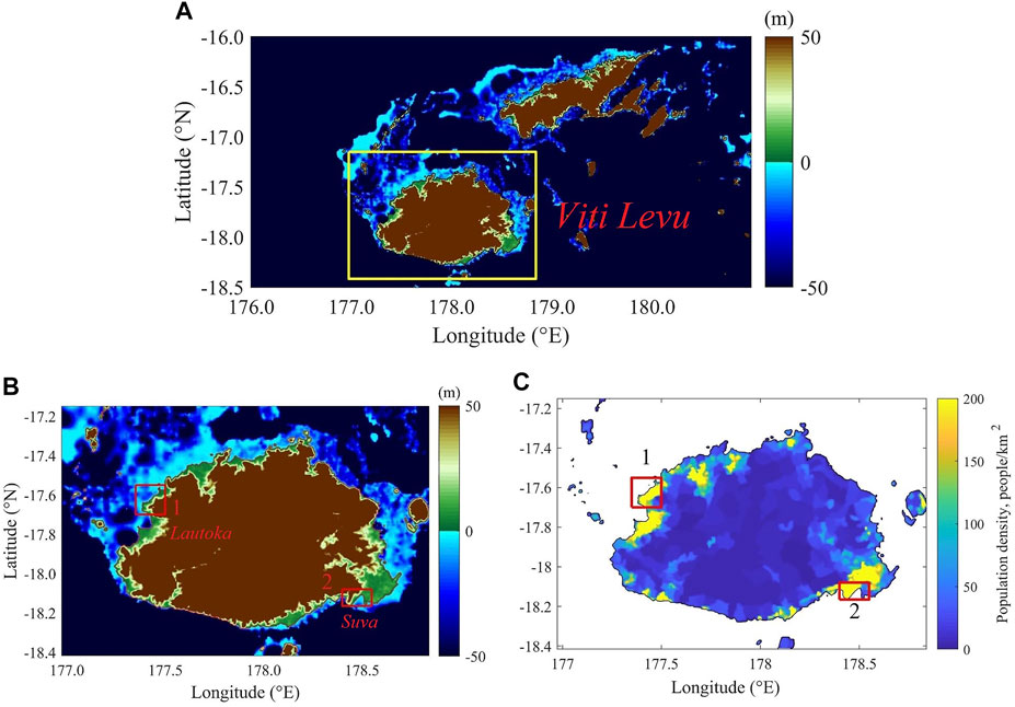
FIGURE 1. Bathymetry and topography data of Fiji with Viti Levu Island selected (A) and its bathymetry and topography (B) and population density map (C) with two most populated areas (unit (C) number of people/km²) (A, B) meters above sea level).

Two low-lying and populated locations are selected for a more thorough analysis to understand the climate change impact on coastal areas with different coastal settings better:

#1. Lautoka area, located 17.62° S, 177.4° E. The number of inhabitants: 59,969.

#2. Suva area, located 18.12° S, 178.5° E. The number of inhabitants: 151,993.

Lautoka represents the northwestern coast of the island, which harbours the second and the third biggest cities in Fiji. It is also an area with a generally shallow water depth near the coast (Figure 1B). In contrast, the Suva area represents the southern coast, surrounded by a deeper ocean. A more shallow ocean creates more suitable conditions for storm surges.

Topography and Social Data

This study used real existing data for topography (landmass data) and bathymetry (ocean data) to project climate change impact on Viti Levu. As for the social input, we used population density data for the Viti Levu estimates. This study used SRTM for topography data input. The SRTM digital elevation model (DEM) provides 3 arcseconds topography data (Jarvis et al., 2008). Meanwhile, GEBCO provided ocean bathymetry data. It is based on a global bathymetric grid with 30 arc-seconds resolution (Becker et al., 2009). In addition, the Gridded Population of the World, Version 4 (GPWv4), created by NASA Socioeconomic Data and Applications Center (SEDAC), provided population density data. It is a raster data collection with an output resolution of 30 arcsec. The dataset includes the population data from the national population and housing censuses conducted between 2005 and 2014. (CIESIN, 2018). All data were interpolated into the same grid size (3 arcseconds) and used in the numerical model. The analysis is based on the records of TCs passing within a 3° radius from the central coordinate of the Viti Levu Island (17.8°S, 178°E). In addition, this study classifies TCs into three groups, depending on their track proximity to the Viti Levu Island: within a 1° radius, within a 2° radius, and within a 3° radius.

The recorded TC data was acquired from the International Best Track Archive for Climate Stewardship (IBTrACS) dataset. The IBTrACS dataset, version v04r00, released by the US National Oceanic and Atmospheric Administration (NOAA) in 2018, is used as source data for the historical TC track information. This study uses information acquired after the introduction of satellite data and updated every 6 h (i.e., starting from the 1978 season) to avoid imprecise results (Tennant, 2004). Furthermore, the TC seasonal convention commonly used in the Pacific region is used, i.e., the TC begins in November of the previous calendar year (Diamond et al., 2013). Data originates from the two datasets, New Zealand MetService and United States Agency information.

Tropical Cyclone Warning Center (TCWC) in Wellington (New Zealand MetService) data is used for the data input between 1978 and 2005. This data contains almost identical data from The WMO Regional Specialised Meteorological Center at Nadi from 1997. Meanwhile, United States Agency information comprised of National Hurricane Center (NHC), Joint Typhoon Warning Center (JTWC), Central Pacific Hurricane Center (CPHC), as well as WMO Regional Specialised Meteorological Center at Miami and Honolulu are used for the newest TCs data (2005–2021) and some TCs for 1988–1993 when the first source does not provide the data. Additionally, the Neumann Southern Hemisphere Dataset, produced by Charles J. Neumann (1925–2017), a consolidated dataset for the Southern Hemisphere, was used when the former two datasets contained no information about storm intensity (Neumann, 1999).

This study assumes that the wind direction corresponds to the direction of the approaching TC in a similar way as Mori et al. (2021) Therefore, the directions from which TCs tend to approach the island are analysed to understand TC features near Viti Levu. For this, an average wind direction (from which the wind blows) was estimated using the average approaching direction of a TC during a 48-h period (6-h intervals) prior to landfall, which was defined to occur when the TC location a was closest to a central point b in Viti Levu Island (17.8°S, 178°E). During each time interval i, the approaching TC direction ${\theta }_i$ was calculated before converting using Eq. 4.

${\theta }_i=\text{arctan}\left(\frac{{\lambda }_i-{\lambda }_{i+1}}{{\varphi }_i-{\varphi }_{i+1}}\right),(4)$

where a_i = (λ_i, φ_i) is the track location in latitude and longitude and a₁ = (λ_1, φ₁) refers to the closest point. Similarly, the average direction $\theta$ for the 48 h period prior to landfall (i.e., time at point ${\theta }_1$) was calculated by first averaging the directional components of ${\theta }_i$, as explained in Eq. 5.

$\left({\theta }_{x,ave}, {\theta }_{y,ave}\right)=\left({\displaystyle \sum }_{k=1}^{n-1}\frac{\cos {\theta }_k}{n-1},{\displaystyle \sum }_{k=1}^{n-1}\frac{\sin {\theta }_k}{n-1}\right),(5)$

Since the IBTrACS dataset usually has data for a TC track every 6 h, n is set to 8. However, if a TC was generated close to Fiji, n may lie between 2 and 7, corresponding to 12 and 42 h before the TC’s approach to the island. TCs formed 6 h or less before landfall on Viti Levu are excluded from the angle analysis, assuming they would not result in floods.

To further simplify the analysis, θ is limited to just twelve main directions ${\theta }_j$ (i.e., Δθ = 30°), with the condition that $-15°< {\theta }_j-{\theta }_i\le +15°$. This condition is essential when calculating a weighted average based on wind angle probability for future climate, as explained in Sea Level Rise Data.

Sea Level Rise Data

SLR and sea level pressure (SLP) were integrated into the model statistically and linearly. SLR values were inputted from the IPCC Special Report on the Ocean and Cryosphere in a Changing Climate (SROCC, 2019). This study projected two scenarios corresponding to mild and extreme radiative forcing values (IPCC Assessment Report 5 (AR5) RCP2.6 and RCP8.5) (IPCC, 2014). IPCC, 2021 AR5 explains the relationship between the SLR and RCPs. According to the SROCC, the projected global mean sea level fluctuates between 0.29–0.59 m and 0.61–1.1 m, depending on the future radiative forcing scenario compared to 1986–2005 (Oppenheimer et al., 2019). This study uses 43 and 84 cm for future scenarios, corresponding to the RCP2.6 and RCP8.5 average values. We chose the RCP2.6 scenario to represent future climate under the scenario, which is the most compatible with the Paris Agreement’s goal. In addition, we selected the RCP8.5 scenario as the opposite scenario, which is likely under the business-as-usual trend.

Dataset Prior to Bias Correction

For the impact assessment of inundation by storm surge and SLR, this study considered both historical records and historical and future estimates. Atmospheric analysis such as Climate Forecast System Reanalysis (CFSR) or European Center for Medium-Range Weather Forecasts Re-Analysis (ERA) product can be used for the extreme TCs estimation. However, the available reanalysis data is too short and not sufficiently accurate for TC events and related storm surges (e.g., Mori and Takemi, 2016). In contrast, synthetic TC models used to increase the number of TC events have estimated extreme TCs and storm surges (e.g., McInnes et al., 2014; Nakajo et al., 2014). These statistical approaches are straightforward approaches used to estimate the intensity and probability of extreme storm surges. However, the computational cost is relatively high due to an enormous number of computations (e.g., 10,000 years simulation). Moreover, the estimation of TCs on small islands can be regarded as a random process. Thus, constant strong winds blowing over the island were assumed to estimate the maximum storm surge heights for a given return period. This approach can estimate the hot spot of the vulnerable areas of the island; however, it neglects the inhomogeneous distribution of the wind fields of TC. Therefore as a first step, we used wind speeds and central pressure values from the d4PDF and d2PDF mega ensemble projections.

d4PDF and d2PDF are sets of large-scale ensemble climate runs, covering 60 years for historical (100 members) and warmer future climate conditions (50–90 members, Mizuta et al., 2017; Fujita et al., 2019). Therefore, the projections for the historical climate and +4K, +2K future climate integrated 6,000, 5,400, and 3,240 years, in the historical climate, d4PDF and d2PD, respectively. Future climate projections assume a constant +2K and +4K global mean atmospheric temperature rise from the pre-industrial period and roughly correspond to conditions at the end of the 21st century under the RCP2.6 and RCP8.5 scenarios. An extremely large climate dataset allows a non-parametric analysis of 50 and 100-years return value extreme events without the need for fitting the data to extreme-value functions.

The SLP reduction affects storm surge height during wind-induced storms. The SLP data was also obtained from the d2PDF and d4PDF projections and integrated into the model. Silvester has defined the relation between this anomaly and surface elevation as (Silvester, 1971):

$S_a=\frac{1013-{\mathit{P}}_{\mathit{c}}}{100}(6)$

where S_a is the surge amplitude (m), and P_c is the pressure at the storm centre, in hPa. The latter relation is often referred to as the inverse barometer effect and indicates an increase in water level by 0.01 m for a decrease by 1 hPa in atmospheric pressure. We are going to refer to the reduction of SLP as a pressure anomaly.

The estimated weakening of TCs, and a consequent decrease in the wind speed and storm surge heights in the future in the Southern hemisphere, including Fiji, was discussed by Mori et al. (2019). It is clear from the data analysis that even though the area around Fiji is known for large-pressure anomalies, a decrease is projected in future climate, particularly in the +4K case, as shown in Figure 2. The decreasing pressure anomaly in the future is related to the weaker TC intensity in the Southern hemisphere. As a result, extreme wind speeds are expected to weaken by 10.7 and 17.8% under the +2K and +4K scenarios, compared to the historical climate conditions as shown in Figure 3. However, despite the weakening trend of the wind speed, the storm speed around Fiji remains the mightiest in the region for extreme wind speeds in the Southern Pacific, with the most prominent ones located in the Coral Sea (latitudes 20°–15° S, and longitudes 150°–160° E), followed by New Caledonia and parts of Vanuatu, both located in between the Coral Sea and Fiji.

FIGURE 2

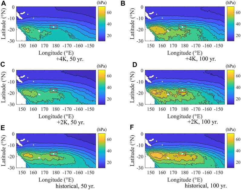
FIGURE 2. Extreme pressure anomalies before bias correction in the case of 50 (A, C, E) and 100-years-return-periods (B, D, F) events in Fiji, under the historical climate conditions (E, F), future climate +2K (C, D), and future climate +4K (a, b, unit: hPa) by the end of the 21st century. A red box indicates the location of Fiji.

FIGURE 3

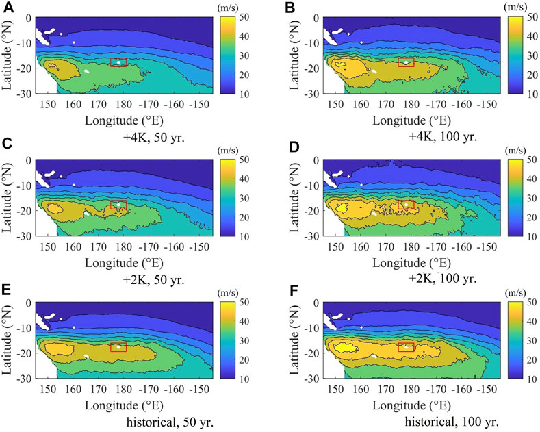
FIGURE 3. Extreme wind speeds in the case of 50 (A, C, E) and 100-years-return-periods (B, D, F) events before bias correction in Fiji, under the historical climate conditions (E, F), future climate +2K (C, D), and future climate +4K (A, B, unit: hPa) by the end of the 21st century. A red box indicates the location of Viti Levu.

Historical TC Data (IBTrACS)

Viti Levu is situated in a location frequently hit by TCs. One hundred one storms having passed within a 3-degree (∼330 km) radius from Viti Levu were tracked between the 1978 and 2021 TC seasons. 44 TCs have passed through Fiji within a 1° radius, 20 passed within a 2° radius and 37 passed within a 3° radius (Figure 4).

FIGURE 4

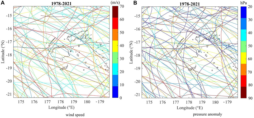
FIGURE 4. Historical TCs that have a record of having passed within a 3° radius from Viti Levu since the 1978 season with (A). maximal wind speed (U₁₀) (unit: m/s) (B). maximal pressure anomaly (unit: hPa).

The study compared storm intensity dynamics for equal periods between 1978 and 2021. The first step in the analysis compared the proximity of the recorded TCs approaching Fiji. The years 1978–1988 had the highest number of the TCs passing nearby Viti Levu, both as a whole and within a radius of 1°. More than one-third of all TCs in 1978–2021 occurred in this period. In contrast, 1989–1999 had the lowest recorded TCs number and the highest proportion of TCs approaching within a 1° radius compared to other periods. Furthermore, the most recent times (2011–2021) are noted for quite a high percentage of the TCs advancing within a 1° radius. 55% of all the recent TCs have approached Viti Levu within this range, constituting 27% of all recorded TCs (Figure 5A). Even though the total number of TCs has decreased compared to 1978–1988, the most recent period (2011–2021) exceeds the TC numbers for 1989–1999, the period noted for the smallest number TCs, more than 1.5 times. Statistically, Viti Levu has been experiencing 1 TC passing within a 1° radius annually (Figure 5B). The numbering convention used (270° (north), 0° (west), 90° (south), and 180° (east)) represents the direction from which the wind is coming. The scheme explaining Eqs 4, 5 is depicted in Figure 5.

While the directional extent is very broad due to Viti Levu’s small size, 74% of all TCs have approached the island from directions ranging between west (0°) and north (270°). Out of these, the TCs approaching the Viti Levu Island from 330° constitute almost one-third of all the recorded TCs, respectively. The number of the cyclones from these two angles exceeds the number of TCs coming from the angles between 180° and 0°, i.e., the southern half, 1.76 times. The northwestern angles are also dominant for the TCs approaching within a 1° radius from Viti Levu (57% of TCs within this range have approached from 330° to 300° angles). Meanwhile, no TC activity between 60° and 120° angles has been recorded according to the available data. Overall, very few TCs approach the island from the southern half, except for a 30° angle (Figure 5B). Instead of assuming that the TC occurrence is equally likely to occur at any point, this study considered the probability of each angle based on the historical records when calculating the averaged value.

FIGURE 5

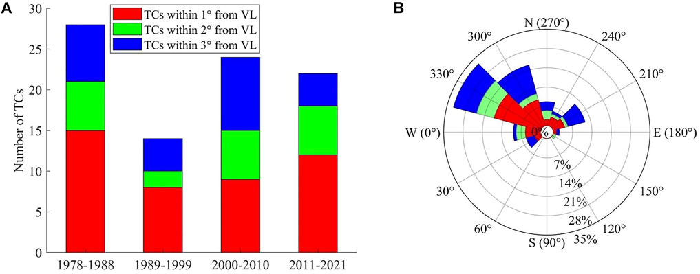
FIGURE 5. TC occurrence frequency by radial distance in Viti Levu (A) per decade, (B) percentage by the angle from which a TC approaches (270° corresponds to the direction from the north (unit: number of TCs, colour: radial distance).

There is a slight decrease in the average annual pressure anomaly, comparing the existing TC records from the 1978–1988 period. The value has fallen by 4.13 hPa, despite very intense storms occurring once in three-four years since 20 years ago (Figure 6A). In addition, the TCs from the 2011–2021 period are 0.8% less intense than the total average. It is also important to note that some missing values in 1978–1988 and 1989–1999, potentially attributable to some weaker TCs, aggravate a better comparison of the TC intensity dynamics. Nevertheless, according to the existing data, 1989–1999 was known for the most intense TCs in terms of pressure. This period has wind speeds 14% above the 2011–2021 average and 14.7% above the total average. Meanwhile, the average central pressure anomaly for 2000–2010 is the lowest, i.e., 13.47% lower than the average of all counted TCs having approached Viti Levu since 1978, considering the available pressure data (Figure 6A). A similar tendency of a decrease, compared to 1978–1988, could be observed for wind speed. The maximum annual wind speed has dropped by 15% compared to 1978 (Figure 6B). This tendency is despite all the strongest wind speeds being recorded over the past 10 years.

FIGURE 6

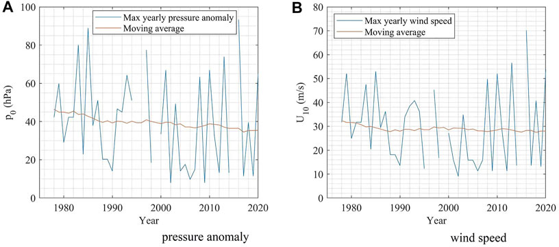
FIGURE 6. Maximum annual pressure anomaly (A) and wind speed (B) around Viti Levu, according to the IBTrACS data. The blue line indicates max yearly pressure anomaly (A) and wind (B), the red line indicates the 40-years moving average (unit (A) m/s (B): hPa).

Despite the general trend for the TCs to decrease in central pressure anomaly, the number of very intense TCs (>60 hPa anomaly) has been increasing with time (Figure 7A). When analysing the angle from where the TCs approach, the storms coming from the most visited 330° angle also tend to be the most intense. 330° and 180° angles are the only ones that have recorded storms with a pressure anomaly of over 80 hPa. When comparing the average central pressure anomaly, rather than the records of the most potent TCs, 180° and 270° angles are known for the most intense TCs on average (51.5 hPa and 43.6 hPa, respectively), despite relatively low occurrences. These numbers exceed the average pressure anomaly by 18.9 hPa and 11 hPa, respectively and the average values for the 330° angle by 13.8 hPa and 5.9 h Pa, respectively. Meanwhile, TCs coming between west and east (30°–150°) are exclusively weak, as their central pressure anomaly has not exceeded 21.2 hPa and has been 17.16 hPa on average. It is also worth noting that the most intense cyclone ever recorded near Viti Levu approached the island from the east, an angle where only 2 TCs affecting Viti Levu have been recorded (Figure 7B). Meanwhile, the least intense recorded cyclone (9.7 hPa) approached from the same eastern angle in the 2011–2021 period (Figures 7A,B).

FIGURE 7

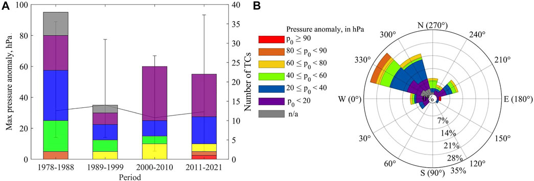
FIGURE 7. TC occurrence frequency and maximum pressure anomaly by period (A) and TC approach angle (B) for 1978–2021 near Viti Levu (bar: number of TCs, line: averaged pressure anomaly, colour: pressure anomaly, error bar: the range of pressure anomaly values for the recorded TCs (unit: hPa).

Extreme Value Analysis and Bias Correction

Extreme value analysis (EVA) is the means of characterising a hazard by estimating the intensity and the frequency of occurrence of the event. EVA is the branch of statistics investigating the extreme deviations from the mean or the median of probability distributions, thus helping to estimate the probability of a certain extreme value to occur. EVA in statistical models for estimating the extreme event frequencies has been used for over 60 years (Dalrymple, 1960; Cunnane, 1987; Hamdi et al., 2021).

EVA was conducted using the annual maximum wind speeds from the IBTrACS and d4PDF historical datasets. We generated generalised extreme value distributions of the extreme wind speed and pressure anomaly return periods, based on the latter datasets.

Before applying bias correction, the probability density function for the generalised extreme value distribution (GEV) was used for the EVA. The results were later used to estimate the distribution of the extreme wind speed, associated to different return periods. The following equation represents the probability density function of GEV with three parameters: location μ, scale σ, and shape k:

$y=f\left(x\text{|}k,\mu ,\sigma \right)=\left(\frac{1}{\sigma }\right)exp\left(-{\left(1+k\frac{(x-\mu )}{\sigma }\right)}^{-\frac{1}{k}}\right){\left(\left(1+k\frac{(x-\mu )}{\sigma }\right)\right)}^{-1-\frac{1}{k}}(7)$

for $1+k\frac{(x-\mu )}{\sigma }>0$, k $\ne 0$, where k > 0 corresponds to the Type II case and k < 0 corresponds to the Type III case. Type I requires a different equation.

Probability density functions are known to have been used to specify the likely distribution of occurrence of variables (Wilks, 2011). We developed cumulative probability functions based on the maximum yearly wind speed values and pressure anomaly values within a 3° radius of Fiji (Figures 8A–C).

FIGURE 8

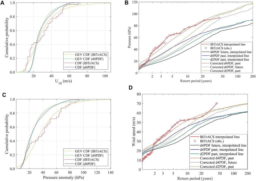
FIGURE 8. Density function and return-period-distribution line graphs of the annual maximum wind speed and pressure anomaly IBTrACS and d4PDF historical datasets: (A), (C)—cumulative distribution function graph comparison between IBTrACS (orange and green lines) and d4PDF (red and blue lines) datasets. (B), (D)—extreme value distribution of annual maximum pressure anomaly (B) and wind speed (D) before (solid lines; black: d4PDF future, blue: d4PDF historical, green: d2PDF future) and after the bias correction (dotted lines; grey: d4PDF, green: d2PDF, orange: historical) against the IBTrACS dataset [solid red line)].

The GEV probability distribution facilitates the analysis between the d4PDF past dataset and the IBTrACS observed data to correct the presumed bias between the historical data. On the other hand, the bias correction based on the GEV distribution has been reported to be complicated from the short records (Carney, 2016). As the data for the bias correction was limited to 42 years, we used a non-parametric method for both storm surge and SLP correction. All data corresponds to the Type II case. Meanwhile, a storm’s most probable wind speed differs by 1.5 m/s between the datasets. The most probable wind speed, based on the d4PDF data, is 21.5 m/s. Meanwhile, the most probable wind speed, based on the IBTrACS records, is 20 m/s. This difference between the datasets is lower than the differences between the extreme speed values between bias-corrected and default datasets. Meanwhile, the comparison of pressure brought more divergent results, i.e., 17 hPa based on the d4PDF data and 28 hPa based on the IBTrACS records.

In addition, we used the Generalised Pareto Distribution (GPD) for the extreme value distribution. The GPD enables to show that at extreme values, the cumulative probability distribution becomes asymptotic to 1, facilitating TC intensity representation (McInnes et al., 2014). The GPD analysis shows that extreme winds over 60 m/s and a pressure anomaly above 80 hPa are rare (Figure 8A and Figure 8C). As seen from Figure 8B and Figure 8D, the maximum magnitude differs slightly between the observational and estimated data. Even though hardly probable, the upper bound of wind speed can reach 100 m/s and 130 hPa of pressure anomaly, according to the IBTrACS dataset vs 75 m/s, and 110 hPa according to the d4PDF mega ensemble dataset. Due to such noticeable differences, a bias correction is needed. The bias correction was applied by shifting d4PDF and d2PDF values by a constant. This constant was derived from the 43-years average of maximum annual and pressure differences. Unlike the mega ensemble datasets, only 43 years of recorded annual maximum wind speeds data for the IBTrACS require fitting the data to extreme-value functions. The values before and after bias correction are presented in Table 1.

TABLE 1

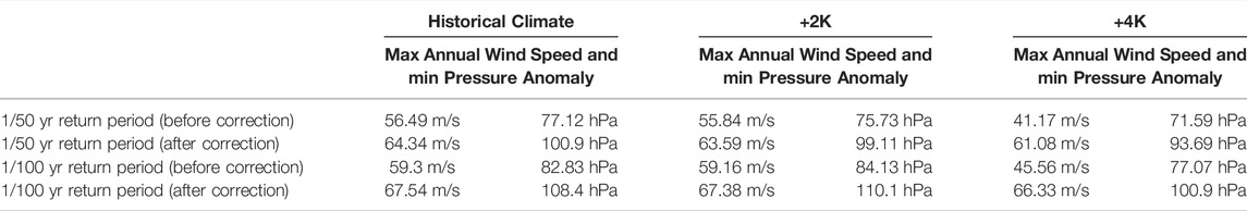
TABLE 1. Extreme wind speed and pressure anomaly value comparison between past and future climate scenarios after applying bias correction.

50-years return value storms. 50-years extreme winds have a 56–89% increase in wind speed and a 112–153% increase in pressure anomalies. Bias correction has the highest impact on the +4K scenario but is less significant for the historical climate. In contrast, the increase is less severe for 100-years return value storms, especially wind speed values. The bias correction increased extreme wind speed values by 48–71% and pressure anomalies by 100–171%. Similar tendencies of an increase with different climate scenarios are observed for 100-years return value storms.

Finally, we calculated the expected values of inundated areas and the population exposed to the inundation during the data analysis under various scenarios. Calculation of the averaged values also took the wind angle probabilities into account. For this reason, the weighted averages, ${\overline{E}}_w$, using a wind angle distribution were calculated with the maximum annual wind speeds and pressure anomalies corresponding to the 50- and 100-years return periods (Figure 2), as defined by Eq. 5:

${\overline{\mathit{E}}}_{\mathit{w}}={\displaystyle \sum }_{\mathit{i}=1}^{\mathit{n}}{\mathit{w}}_{\mathit{i}}{\mathit{E}}_{\mathit{i}}(8)$

where $w_i$ is the probability of a certain wind direction ${\theta }_i=\left(i-\frac{1}{2}\right)360/n$ from which the storm approaches, n the number of directions, and $E_i$ the expected value for the direction ${\theta }_i$. We used these weighted averages for analysing inundation, population exposed to the inundation, and surface elevation in coastal areas.

As seen from the table, bias correction has resulted in a significant increase of 100- and particularly 50-years return value wind speed and pressure values.

Results

Projected Storm Surge Heights Before and After Bias Correction

We started our analysis with the storm surge heights simulations during extreme storms. Storm surge impact from the point of view of the sea surface elevation was previously assessed by McInnes et al. (2014). However, this study also analysed the difference between non-corrected and corrected climate data in addition to the projected values for the extreme events during the current and future climate. Figure 9 compares spatial distribution before and after the bias correction. While surges near the coast rarely exceeded 3 m for the models with no bias correction, these values were more than 5 m after the bias correction. However, the most efficient way to check the differences is by selecting and comparing certain coastal points. For that reason, the two most affected locations in the northwestern and southern parts were selected.

FIGURE 9

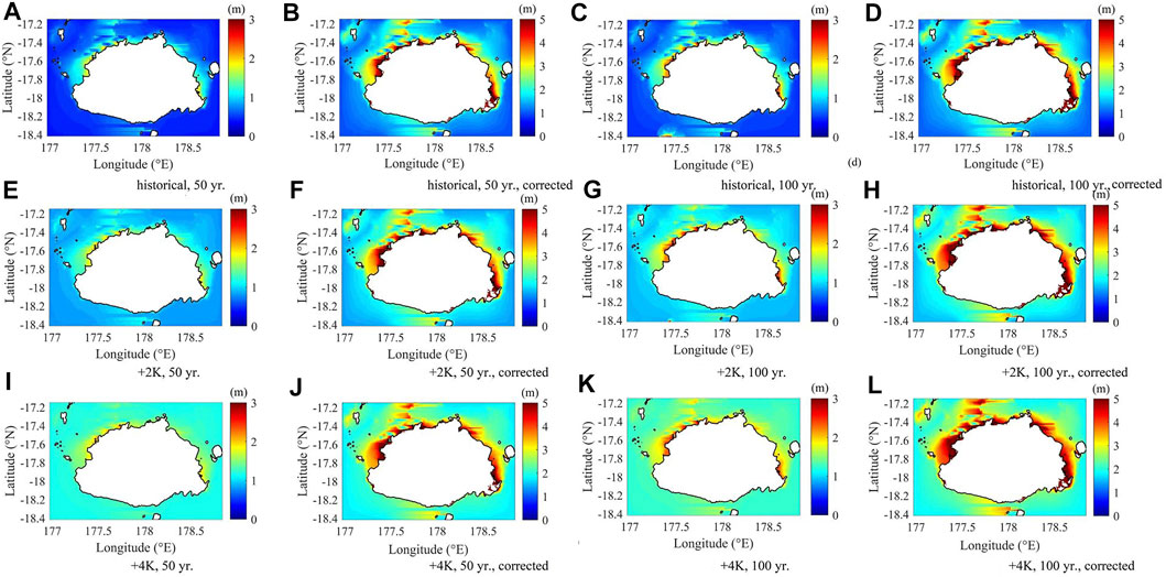
FIGURE 9. Spatial distribution of the maximum storm surge level combining different probable wind directions before (A, B, E, F, I, J) and after (C, D, G, H, K, L) bias correction for 50- and 100-years extreme wind speed scenario under historical (A, B, C, D), +2K (E, F, G, H), +4K (I, J, K, L) climate conditions (contour–shoreline under current MSL, unit–m above current MSL).

When comparing the results for the two locations, it becomes clear that bias correction makes a big difference, particularly when assessing historical climate conditions. In the case of 50-years-return value storms, the highest averaged value is 3.62 m for Location #1 and 1.8 m for Location #2. However, depending on the wind directions, storm surge heights in these areas can reach between 1.71 and 4.96 m and between 1.71 and 3.78 m, respectively. The effect is 1.5–2.28 times larger than the original values (1.59 and 1.23 m, Figure 10A). In comparison, in the case of 100-years-return value storms, the averaged value is projected to be up to 4 m for Location #1 and 1.84 m for Location #2. However, depending on the wind directions, storm surge heights in these areas can fluctuate between 1.78 and 5.81 m and between 1.78 and 4.02 m, respectively. An additional effect is 1.8–2.17 times larger after bias correction, especially for the winds under the current climate conditions, compared to the original values (1.25 and 2.22 m). Furthermore, the difference between corrected and non-corrected scenarios fluctuates for Location #2, which faces more moderate storm surges (1.44–2.5 times larger averaged values, Figure 10B). Furthermore, the ratio between 100- and 50-return periods is higher for original than for bias-corrected scenarios.

FIGURE 10

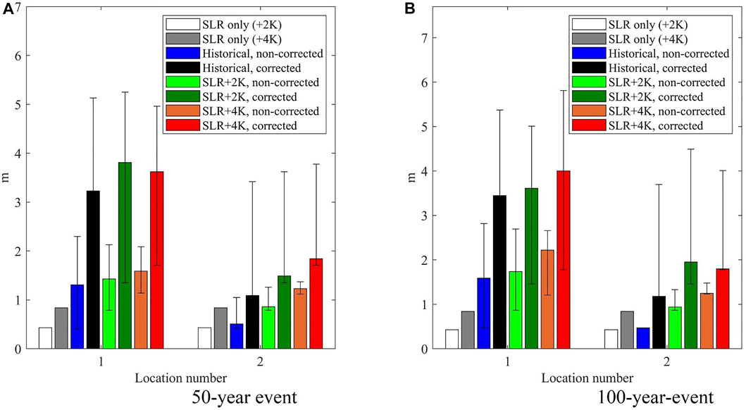
FIGURE 10. Maximum surface elevation height in coastal locations #1 and #2 for a 50- (A) and 100- year (B) extreme event (bars: weighted average surface elevation height under different SLR (white and grey) and cumulative SLR and surge (blue to red) scenarios) and spatial distribution under varying wind angles; unit: m).

Compounding Effects Impact on Inundation and Population

In the next step, we estimated the inundated area scope due to the compounding effects of SLR and storm surges. Meanwhile, the number of studies that assessed inundated areas is more limited than the projected total sea surface elevation. Firstly, the anticipated inundation scope is projected for the current and past climates, and the results are compared between different storm magnitudes and before and after bias correction. Secondly, individual effects of storm surge and sea level rise are calculated. The inundation which cannot be attributed to either component is considered residual effects. The residual effects (RE) are calculated by subtracting the compounding effects (CE), SLR, and storm surge (S) individual effects (Figure 9).

$RE=CE-SLR-S(9)$

RE is attributable to peculiarities in a coastal topography, such as spatial dependence of coastal slopes. They can also provide information about possible limitations (errors) in a model. The peculiarities of the impact of each component are further discussed in Subsection 3.4.

The largest weighted average inundation is projected for 100-years return value storms under the +4K future climate scenario (158 km², or 1.5% of the islands’ territory). Meanwhile, the weighted averages fluctuate between 147 and 158 km² between different climate scenarios. In the case of a 50-years extreme event, the weighted average inundation is 17% lower under the +4K climate (Figure 11A). The ratio of projected inundation area is 1.98–3.38 times larger between non-bias corrected and bias-corrected scenarios for 50-years events (Figure 11A). Meanwhile, bias-corrected and non-bias corrected scenarios-based inundated areas differ 2.12–3.2 times for 100-years events (Figure 11B). As one may see, there is a higher fluctuation compared to the 100-years storm bias correction (a wider gap between the extreme values).

FIGURE 11

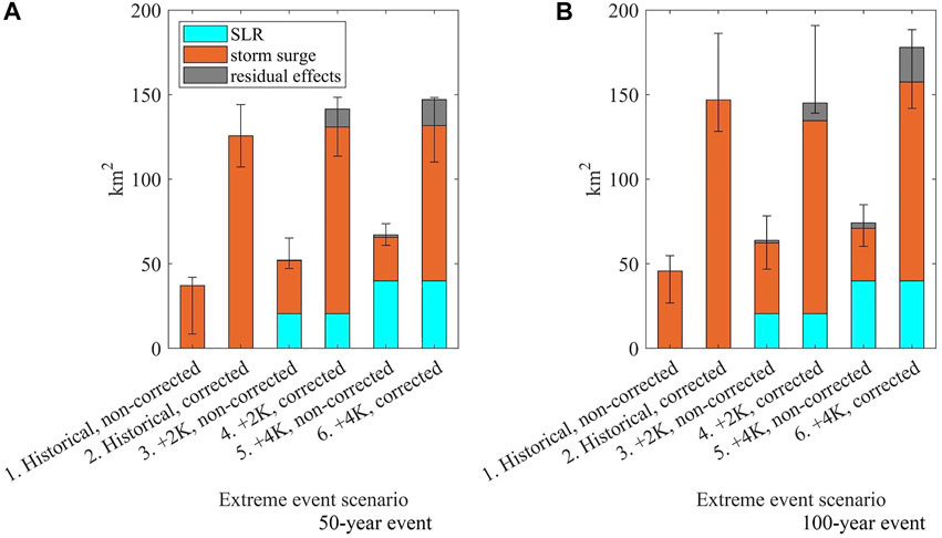
FIGURE 11. Weighted average values of inundated areas under different climate scenarios and before and after the correction (1/50 (A) and 1/100 (B) winds under the +4K, +2K, and historical climate conditions), indicating the contribution of SLR and storm surge (error bars: inundation fluctuation depending on the wind direction; unit: km²).

Next, we projected the number of exposed populations living in the inundated areas and compared the differences between original and bias-corrected projections. The largest weighted average of the exposed population for a 100-years event is projected to occur under the +2K future climate scenario (2.4% of the islands’ population). The estimates differ by only 2% between different climate scenarios. Such a slight difference contrasts to non-corrected scenarios and 50-years events where the differences are more considerable. Meanwhile, considerable differences exist depending on the wind angle–the exposed population estimates differ 2.35 times if a 100-years TC makes landfall on the western shore rather than the eastern one (Figure 11).

As we saw from the previous sections, a bias correction increases the projections more than two times. However, these changes are even more dramatic for the exposed population estimates. The exposed population estimates increase 2.62–4.47 times compared to non-corrected values. For 50-years storms, +4K correction yields the most significant results (Figure 12A). The bias-corrected and non-bias corrected scenarios-based inundated areas differ 3.2–4.97 times. The difference is the smallest for the +4K climate scenario (Figure 12B). As in the case of inundated areas projections, there is a higher fluctuation than the 100-years storm bias correction.

FIGURE 12

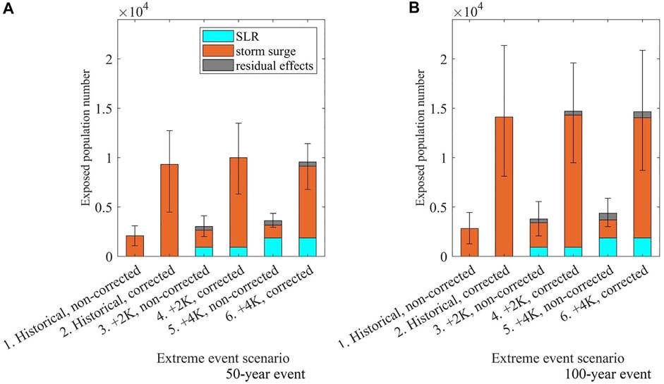
FIGURE 12. Weighted average values of the population numbers exposed to inundation under different climate scenarios before and after the correction (50- (A) and 100-years (B) extreme events under the +4K, +2K, and historical climate conditions), indicating the contribution of SLR and storm surge (error bars: inundation fluctuation depending on the wind direction).

Effects of Individual Components

This section investigates the role of SLR, storm surges and residual effects in the final projection of total inundation in three climate scenarios (historical, +2K, +4K) under 1/50 and 1/100 return period wind speeds, with and without bias correction. In addition, SLP, which increases sea surface heights effect during the storm surges, is also listed separately. SLP is a crucial factor responsible for more devastating storm surge effects and worsens total sea surface elevation due to the barometer effect. The value for SLP was attributed by subtracting the total inundated area, considering the barometric effect of pressure anomaly and inundation size projected with a storm surge alone.

As seen in Figure 13 as well as Figures 11, 12, a ratio of storm surge contribution to total inundation is the most significant component for the land inundation during the most extreme events in the future climate. Depending on whether bias correction was applied or not, the proportion of the SLR and storm surge contribution differs significantly. This difference can be attributed to the increased extreme wind magnitude after bias correction, leading to a broader inundation scope. In the case of a non-bias-corrected 50-years event, the SLR contribution is more important than the storm surge contribution. Its role is less critical only for the storms without bias correction. Meanwhile, SLP is the most impactful in the +2K climate. It can be attributed to the fact that more intense storms are projected for the +2K scenario than the +4K climate; therefore, the values of storm-induced pressure are correspondingly higher. Furthermore, the contribution of SLP is the most pronounced under less intense 1/50 years return value winds (Figure 13A). It is also an essential component for the storms under historical climate even though its ratio falls as the storm increases. Meanwhile, in the case of the corrected 1/100 years return value events under the +4K climate, the SLP effects become negligible, as their contribution is lower than residual effects (the latter, however, have negative values, Figure 13B).

FIGURE 13

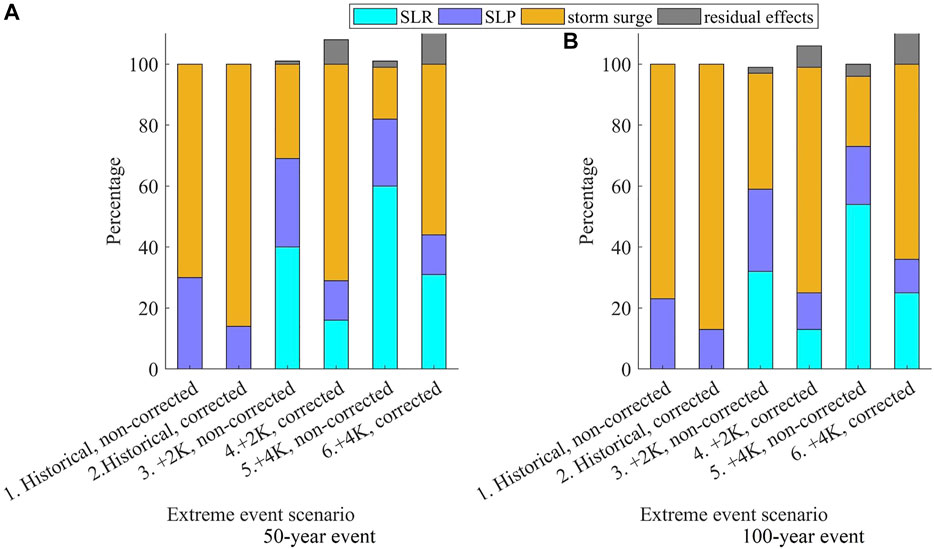
FIGURE 13. Contribution of different compounding effects factors to inundation area for a 50- (A) 100-years (B) event under the historical, +2K, and +4K climate conditions before and after the bias correction; black bar: SLR, blue bar: SLP, violet bar: storm surge effects alone, grey bar: residual values (unit: %)). Some residual values were negative; therefore, the storm under +2K and +4K bars had values beyond 100%.

In addition to general trends, exposed population number estimates were projected for two coastal locations on the island (refer to Figure 1 for the locations). 50- and 100-years return period storms are equally impactful for Location 1, irrespective of the climate scenario. 50-years return value storms can expose 3,700–3,780 or 6.15%–6.3%, 100-years return value storms can expose 3,900–4,050, or 6.5–6.75%, of the local population. Meanwhile, the differences between climate scenarios are more significant for Location 2, but even the most extreme storm is not projected to affect more than 0.5% of the local coastal population. In this location, as on the southern coast in general, SLR plays a relatively significant role as a component, accounting for 40% of the total inundation (Figure 14).

FIGURE 14

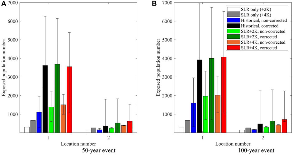
FIGURE 14. Exposed population numbers in locations #1 and #2 in the case of a 50- (A) and a 100-years (B) extreme event compared to the effect of the SLR only (bars: weighted average under various SLR (white and grey) and cumulative SLR and surge (blue to red) scenarios; error bars–inundation fluctuation depending on the wind direction).

In addition, the role of a bias correction for the projections of the two coastal locations was evaluated. The results were as follows: the exposed population for Location 1 increased 2.36–3.26 times, while for Location 2, the difference was between 1.58 and 2.33 times for a 50-years extreme event, as shown in Figure 14A. Meanwhile, estimates for the 100-years return period storm are 2–2.45 times higher for Location 1 and 1.68–2.82 times higher for Location 2 after bias correction, as Figure 14B indicates. The difference is huge for the historical climate but relatively less significant for the storms for the +4K climate. Overall, the difference is lower for Location 1 but higher for Location 2 than the 50-years storms.

Discussions

Even though a bias correction helps make more realistic projections in the case of extreme events the impact on the population is quite low and appropriate adaptive measures may prevent the population from a mass-scale displacement. On the other hand, the results after the bias correction highlight more vulnerable regions, as an increase in the inundated areas is particularly sharp for the western and northwestern part of the Viti Levu Island. While the bias correction does not affect the sea level rise projections, it also points out the significance of the storm surges in the compounding effects under the future climate due to a dramatic increase of the wind speeds for the 50- and 100-years return extreme events. In addition, the effects of 100-years extreme events are very similar irrespective of the climate scenario after the bias correction in contrast to the projections without a bias correction where the difference between different radiative forcing scenarios even for 100-years return period storms is clear.

Even though a precise comparison would require the application and recalculation of the storm surges for other islands in Fiji, the results from Viti Levu and analysis of Figures 2, 3 allows us to conclude that many other islands in Fiji and other volcanic islands in the region are susceptible to the compounding effect of sea level rise and storm surge. In addition to most islands of Fiji, Vanuatu and New Caledonia (both situated west of Fiji) are also located in cyclonically active areas and consist of either volcanic or continental islands. Historical evidence shows that these islands could also face similar consequences as Viti Levu (International Federation of Red Cross And Red Crescent Societies, 2015; European Commission’s Directorate-General for European Civil Protection and Humanitarian Aid Operations, 2021). Therefore the results of this study can build a better understanding of the situation of the volcanic islands in the South Pacific as climate change proceeds.

As documented from the past TCs, extreme events can result in huge economic loss for Fiji or other affected islands. However, the consequences of compounding effects can be limited not only to the economy. Climate change can also negatively affect biological diversity. For instance, compounding effects threaten tropical dry forests located in the western and northern parts of Viti Levu, the most vulnerable spots on the island. As such, the compounding effects may negatively affect the potentially highly endangered plant species (Cynometra falcata and Guettarda wayaensis) (Taylor and Kurmar, 2016). Other negative consequences of climate change could be traditional knowledge loss or even a negative impact on endangered languages, as biodiversity and language diversity are intertwined (Amano et al., 2014; Sabūnas et al., 2021). There are a few endangered species, which are susceptible to climate change on Viti Levu. In contrast, the main languages used in Fiji, Fijian and Fijian Hindi, are considered vital and thus are not affected by migration. The only endangered local language is Rotuman, spoken in the Rotuma Island, ∼650 km north of Viti Levu (Moseley, 2010). However, Rotuma is affected by significantly weaker TCs than Viti Levu. Therefore this study is unable to make even rough estimates of its situation.

This study used the future sea level rise estimates from the SROCC (SROCC, 2019). Meanwhile, the most recent assessment report released in 2021 projects slightly lower median values for the year 2050 and the year 2,100 in particular (−1 cm and −7 cm respectively) (IPCC, 2021). However, the differences are negligible given the fact that Viti Levu Island is a high island where storm surges play a more significant role in the compounding effects. Meanwhile, it is worth taking into account that the sea level rise projection does not consider the newest evidence regarding mass balance of the Greenland ice sheet which is not a part of the newest IPCC report but which may elevate the future sea level rise projections (Shepherd et al., 2020).

Even though other studies have applied bias correction, few studies exist to compare the impact of the bias correction on numerical models of the future climate (Carney, 2016). The bias correction can improve the model uncertainty arising due to a coarse resolution of a GCM and a method to consider a constant wind speed and direction. On the other hand, the correction cannot address the scenario uncertainty and the internal variability. Because of the bias correction application and the SLP effect consideration, the total sea surface elevation projections, inundated areas, and exposed population numbers during the extreme events were higher than projected in an earlier study by Sabūnas et al. (2020). The inundated areas were 1.8 times higher and exposed population numbers were up to 2.65 times higher than the projections without a bias correction Sabūnas et al. (2020). Meanwhile, sea surface estimates for 100-years extreme winds were higher in this study than McInnes et al. (2014). This seemingly conflicting finding could also be attributed to a bias correction method and different coastal locations between the studies.

This study applied bias correction while treating each variable independently. Despite this, we can spot a clear correlation between two variables, the wind speed and SLP, which are closely related parameters defining the TC intensity. Meanwhile, some studies have considered joint bias (precipitation and temperature) corrections in an attempt to reduce biases in the mean and variance of each variable (Li et al., 2014). However, our study did not consider a bivariate bias correction as this type of bias correction could have led to higher errors for the extreme wind speeds whose values would have increased. This would result in higher exposure estimates for both historical and future climate conditions.

Conclusion

Small island developing states, such as Fiji, contribute little to the global greenhouse gas emissions but will experience disproportionate consequences of climate change. Some coastal areas in Fiji are affected by compounding effects and could suffer tremendous economic loss, even more so in the future. On the other hand, relatively low exposure numbers mean only a limited islands’ population is threatened. Furthermore, most of the threatened population is subject to temporary displacement. Only 0.31% of the island’s population could be permanently displaced solely due to the SLR effects. Owing to such a small number and the island’s size, it is quite unlikely that climate-related events may displace a more significant number of the population out of the island. On the other hand, a future SLR acceleration will result in more devastating extreme events for Fiji coastal population.

Depending on future climate scenarios, 100-years return value storms may inundate 1.5% of the island’s territory and affect 2.4% of the island’s population. In addition, some coastal areas may exhibit surface elevation as high as 5.8 m (compared to the current MSL) during the 100-years storms in the future. However, the vulnerability is place-dependent, and most exposed people are estimated to be from the west and northwest coast of Viti Levu. In addition, there are significant differences in projections depending on whether we use bias-corrected data or not, particularly for the displaced population and for the +4 K climate scenarios. However, it is hard to draw a clear linear relation between magnitude and population displacement. For instance, Cyclone Harold is attributable to a 10-years-return period event for Viti Levu but displaced only 0.11% of the island’s population, fewer than estimated. Meanwhile, Cyclone Winston is attributable to a 100-years-return period event but displaced 6.2%, higher than the estimates. Therefore, more accurate estimates of the displacement scopes would require creating a vulnerability map to distinguish the exposed population from the displaced population.

This study concludes that despite the decrease in wind speed and an increase in the central pressure of the TCs under future climate, a faster pace of climate change means a more critical vulnerability level for Fiji. Therefore, the adaptive capacity of Fiji and success or failure not to exceed the warming by 2° globally may be the forces that would determine the impact of future TC in Fiji.

Data Availability Statement

The raw data supporting the conclusions of this article will be made available by the authors, without undue reservation.

Author Contributions

Numerical simulation, validation, analysis of the results, preparation of the manuscript, structure, revisions (AS); initial SWE storm surge model, structure, revisions (NM); d2PDF, d4PDF data input, modifications (TS); improving the SWE storm surge code (NF); model improvements (TM).

Funding

A part of this research is supported by the Integrated Research Program for Advancing Climate Models (TOUGOU) Grant Number JPMXD0717935498 by the Ministry of Education, Culture, Sports, Science, and Technology (MEXT) and the Climate Adaptation Program in NIES and JSPS Grant-in-Aid for Scientific Research (Kakenhi).

Conflict of Interest

The authors declare that the research was conducted in the absence of any commercial or financial relationships that could be construed as a potential conflict of interest.

Publisher’s Note

All claims expressed in this article are solely those of the authors and do not necessarily represent those of their affiliated organizations, or those of the publisher, the editors and the reviewers. Any product that may be evaluated in this article, or claim that may be made by its manufacturer, is not guaranteed or endorsed by the publisher.

Acknowledgments

AS would like to express utmost gratitude to the Ministry of Education, Culture, Sports, Science and Technology of Japan (MEXT) for providing with a scholarship, and the Climate Change Adaptation Research Program of NIES. The authors are also grateful to Adrean Webb for improving the angle calculating equations.

References

Amano, T., Sandel, B., Eager, H., Bulteau, E., Svenning, J.-C., Dalsgaard, B., et al. (2014). Global Distribution and Drivers of Language Extinction Risk. Proc. R. Soc. B. 281, 20141574. doi:10.1098/rspb.2014.1574

PubMed Abstract | CrossRef Full Text | Google Scholar

Becker, J. J., Sandwell, D. T., Smith, W. H. F., Braud, J., Binder, B., Depner, J., et al. (2009). Global Bathymetry and Elevation Data at 30 Arc Seconds Resolution: SRTM30_PLUS. Mar. Geodesy 32 (4), 355–371. doi:10.1080/01490410903297766

CrossRef Full Text | Google Scholar

Bettencourt, S. U., Croad, R., Freeman, P., Hay, J., Jones, R., King, P., et al. (2006). “Not if but when: Adapting to Natural Hazards in the Pacific Islands Region - a Policy Note,” in The World Bank East Asia and Pacific Region, Pacific Islands Country Management Unit. (Washington, D. C.: The World Bank).

Google Scholar

Carney, M. C. (2016). Bias Correction to GEV Shape Parameters Used to Predict Precipitation Extremes. J. Hydrol. Eng. 21 (10), 04016035. doi:10.1061/(ASCE)HE.1943-5584.0001416

CrossRef Full Text | Google Scholar

IPCC (2014). “Summary for Policymakers,” in Climate Change 2014: Impacts, Adaptation, and Vulnerability. Contribution of Working Group II to the Fifth Assessment Report of the Intergovernmental Panel on Climate Change, Vol Part A: Global and Sectoral Aspects. Editors C. B. Field, V. R. Barros, D. J. Dokken, K. J. Mach, M. D. Mastrandrea, T. E. Biliret al. (Cambridge, UK: Cambridge University Press).

Google Scholar

Center for International Earth Science Information Network (Ciesin) (2018). Documentation for the Gridded Population of the World, Version 4 (GPWv4), Revision 11 Data Sets. Palisades, NY: NASA Socioeconomic Data and Applications Center (SEDAC), Columbia University.

Google Scholar

Cunnane, C. (1987). “Review of Statistical Models for Flood Frequency Estimation,” in Hydrologic Frequency Modeling. Editor V. P. Singh (Dordrecht: Springer), 49–95. doi:10.1007/978-94-009-3953-0_4

CrossRef Full Text | Google Scholar

Dalrymple, T. (1960). Flood-frequency Analyses, Manual of Hydrology: Part 3.” in Manual of Hydrology: Flood-Flow Techniques. Washington: Geological Survey Water-Supply. doi:10.3133/wsp1543A

CrossRef Full Text | Google Scholar

Diamond, H. J., Lorrey, A. M., and Renwick, J. A. (2013). A Southwest Pacific Tropical Cyclone Climatology and Linkages to the El Niño-Southern Oscillation. J. Clim. 26 (1), 3–25. doi:10.1175/JCLI-D-12-00077.1

CrossRef Full Text | Google Scholar

European Commission's Directorate-General for European Civil Protection and Humanitarian Aid Operations (2021). New Caledonia - Tropical Cyclone NIRAN Update (GDACS, Meteo NC, FranceInfo NC, media) (ECHO Daily Flash of March 8, 2021). Available at: https://reliefweb.int/report/new-caledonia-france/new-caledonia-tropical-cyclone-niran-update-gdacs-meteo-nc-franceinfo-nc. (accessed March 7, 2022).

Google Scholar

Flather, R. A., and Tippett, L. H. C. (1984). A Numerical Model Investigation of the Storm Surge of 31 January and 1 February 1953 in the North Sea. Q.J R. Met. Soc. 110, 591–612. doi:10.1002/qj.49711046503

CrossRef Full Text | Google Scholar

Fujita, M., Mizuta, R., Ishii, M., Endo, H., Sato, T., Okada, Y., et al. (2019). Precipitation Changes in a Climate with 2‐K Surface Warming from Large Ensemble Simulations Using 60‐km Global and 20‐km Regional Atmospheric Models. Geophys. Res. Lett. 46 (1), 435–442. doi:10.1029/2018GL079885

CrossRef Full Text | Google Scholar

Hamdi, Y., Haigh, I. D., Parey, S., and Wahl, T. (2021). Preface: Advances in Extreme Value Analysis and Application to Natural Hazards. Nat. Hazards Earth Syst. Sci. 21, 1461–1465. doi:10.5194/nhess-21-1461-2021

CrossRef Full Text | Google Scholar

Holland, G. J. (1997). The Maximum Potential Intensity of Tropical Cyclones. J. Atmos. Sci. 54 (21), 2519–2541. doi:10.1175/1520-0469(1997)054<2519:tmpiot>2.0.co;2

CrossRef Full Text | Google Scholar

SROCC (2019). in Special Report on the Ocean and Cryosphere in a Changing Climate. Editors H. O. Pörtner, D. C. Roberts, V. Masson-Delmotte, P. Zhai, M. Tignor, E. Poloczanskaet al.

Google Scholar

Internal Displacement Monitoring Center (2021). Fiji. Internal Displacement Monitoring Center. Available at: https://www.internal-displacement.org/countries/fiji (accessed March 7, 2022).

Google Scholar

International Federation of Red Cross And Red Crescent Societies (2015). Pacific: Tropical Cyclone Pam (MDR55001) Emergency Plan of Action Final Report. Available at: https://reliefweb.int/sites/reliefweb.int/files/resources/MDR55001efr.pdf (accessed March 7, 2022).

Google Scholar

Jarvis, A., Reuter, H., Nelson, A., and Guevara, E. (2008). Hole-Filled Seamless SRTM Data V4. International Centre for Tropical Agriculture (CIAT). Retrieved from: http://srtm.csi.cgiar.org/.

Google Scholar

Kostaschuk, R., Terry, J., and Raj, R. (2001). Tropical Cyclones and Floods in Fiji. Hydrological Sci. J. 46 (3), 435–450. doi:10.1080/02626660109492837

CrossRef Full Text | Google Scholar

Lemos, G., Menendez, M., Semedo, A., Camus, P., Hemer, M., Dobrynin, M., et al. (2020). On the Need of Bias Correction Methods for Wave Climate Projections. Glob. Planet. Change 186, 103109. ISSN 0921-8181. doi:10.1016/j.gloplacha.2019.103109

CrossRef Full Text | Google Scholar

Li, C., Sinha, E., Horton, D. E., Diffenbaugh, N. S., and Michalak, A. M. (2014). Joint Bias Correction of Temperature and Precipitation in Climate Model Simulations. J. Geophys. Res. Atmos. 119 (2313), 153–213. doi:10.1002/2014jd022514

CrossRef Full Text | Google Scholar

Little, C. M., Horton, R. M., Kopp, R. E., Oppenheimer, M., Vecchi, G. A., and Villarini, G. (2015). Joint Projections of US East Coast Sea Level and Storm Surge. Nat. Clim Change 5, 1114–1120. doi:10.1038/nclimate2801

CrossRef Full Text | Google Scholar

Mansur, A., Doyle, J., and Ivaschenko, O. (2017). Social Protection and Humanitarian Assistance Nexus for Disaster Response: Lessons Learnt from Fiji's Tropical Cyclone Winston. Washington, DC: World Bank GroupWorld Bank. Social Protection & Labor Discussion paper; no. 1701.

Google Scholar

McInnes, K. L., Walsh, K. J. E., Hoeke, R. K., O’Grady, J. G., Colberg, F., and Hubbert, G. D. (2014). Quantifying Storm Tide Risk in Fiji Due to Climate Variability and Change. Glob. Planet. Change 116, 115–129. doi:10.1016/j.gloplacha.2014.02.004

CrossRef Full Text | Google Scholar

Mizuta, R., Murata, A., Ishii, M., Shiogama, H., Hibino, K., Mori, N., et al. (2017). Over 5,000 Years of Ensemble Future Climate Simulations by 60-km Global and 20-km Regional Atmospheric Models. Bull. Am. Meteorol. Soc. 98, 1383–1398. doi:10.1175/BAMS-D-16-0099.1

CrossRef Full Text | Google Scholar

Mori, N., Ariyoshi, N., Shimura, T., Miyashita, T., and Ninomiya, J. (2021). Future Projection of Maximum Potential Storm Surge Height at Three Major Bays in Japan Using the Maximum Potential Intensity of a Tropical Cyclone. Climatic Change 164, 25. doi:10.1007/s10584-021-02980-x

CrossRef Full Text | Google Scholar

Mori, N., Kjerland, M., Nakajo, S., Shibutani, Y., and Shimura, T. (2016). Impact Assessment of Climate Change on Coastal Hazards in Japan. Hydrological Res. Lett. 10 (3), 101–105. doi:10.3178/hrl.10.101

CrossRef Full Text | Google Scholar

Mori, N. (2012). “Projection of Future Tropical Cyclone Characteristics Based on Statistical Model,” in Cyclones Formation, Triggers and Control. Editors K. Oouchi, and H. Fudeyasu (NewYork, USA: Nova Science Publishers), 249–270.

Google Scholar

Mori, N., Shimura, T., Yoshida, K., Mizuta, R., Okada, Y., Fujita, M., et al. (2019). Future Changes in Extreme Storm Surges Based on Mega-Ensemble Projection Using 60-km Resolution Atmospheric Global Circulation Model. Coastal Eng. J. 61, 295–307. doi:10.1080/21664250.2019.1586290

CrossRef Full Text | Google Scholar

Mori, N., and Takemi, T. (2016). Impact Assessment of Coastal Hazards Due to Future Changes of Tropical Cyclones in the North Pacific Ocean. Weather Clim. Extremes 11, 53–69. doi:10.1016/j.wace.2015.09.002

CrossRef Full Text | Google Scholar

Moseley, C. (2010). Atlas of the World's Languages in Danger. 3rd edn. Paris: UNESCO Publishing. Online version Available at: http://www.unesco.org/culture/en/endangeredlanguages/atlas (accessed March 7, 2022).

Google Scholar

Muis, S., Verlaan, M., Winsemius, H. C., Aerts, J. C. J. H., and Ward, P. J. (2016). A Global Reanalysis of Storm Surges and Extreme Sea Levels. Nat. Commun. 7, 11969. doi:10.1038/ncomms11969

PubMed Abstract | CrossRef Full Text | Google Scholar

Nakajo, S., Mori, N., Yasuda, T., and Mase, H. (2014). Global Stochastic Tropical Cyclone Model Based on Principal Component Analysis and Cluster Analysis. J. Appl. Meteorology Climatology 53, 1547–1577. doi:10.1175/JAMC-D-13-08.1

CrossRef Full Text | Google Scholar

Neumann, J. C. (1999). The HURISK Model: An Adaptation for the Southern Hemisphere (A User's Manual). Miami, FL: Science Applications International Corporation, 31.

Google Scholar

Nunn, P. D., Kumar, L., Eliot, I., and McLean, R. F. (2016). Classifying Pacific Islands. Geosci. Lett. 3, 7. doi:10.1186/s40562-016-0041-8

CrossRef Full Text | Google Scholar

Oppenheimer, M., Glavovic, B. C., Hinkel, J., van de Wal, R., Magnan, A. K., Abd-Elgawad, A., et al. (2019). “Sea Level Rise and Implications for Low-Lying Islands, Coastal Areas, and Communities,” in IPCC Special Report on the Ocean and Cryosphere in a Changing Climate. Editors Pörtner, H.-O., Roberts, D. C., Masson-Delmotte, V., Zhai, P., Tignor, M., Poloczanska, E., et al. (Cambridge University Press: Cambridge, United Kingdom and New York, NY). doi:10.1017/9781009157964.006

CrossRef Full Text | Google Scholar

Price, J. F. (1981). Upper Ocean Response to a hurricane. J. Phys. Oceanogr. 11, 1532–2175. doi:10.1175/1520-0485(1981)011<0153:uortah>2.0.co;2

CrossRef Full Text | Google Scholar

Sabūnas, A., Mori, N., Fukui, N., Miyashita, T., and Shimura, T. (2020). Impact Assessment of Climate Change on Storm Surge and Sea Level Rise Around Viti Levu, Fiji. Front. Clim. 2, 19. doi:10.3389/fclim.2020.579715

CrossRef Full Text | Google Scholar

Sabūnas, A., Mori, N., Shimura, T., Fukui, N., Miyashita, T., and Webb, A. (2021). Assessing Social Impact of Storm Surge and Sea Level Rise Compound Effects in Viti Levu, Fiji, Comparing with the Historical TCs Records. J. Jpn. Soc. Civil. Eng. Ser. B2. 77, 943. doi:10.2208/kaigan.77.2I943

CrossRef Full Text | Google Scholar

Shepherd, A., Ivins, E., Rignot, E., Smith, B., van den Broeke, M., Velicogna, I., et al. (2020). Mass Balance of the Greenland Ice Sheet from 1992 to 2018. Nature 579, 233–239. doi:10.1038/s41586-019-1855-2

PubMed Abstract | CrossRef Full Text | Google Scholar

Silvester, R. (1971). “Computation of Storm Surge,” in Proceedings of the 12th Conference on Coastal Engineering (Washington, UnitedNew York, ASCE, 1, 121. doi:10.9753/icce.v12.121

CrossRef Full Text | Google Scholar

Taylor, S., and Kumar, L. (2016). Global Climate Change Impacts on Pacific Islands Terrestrial Biodiversity: A Review. Trop. Conservation Sci. 9, 203–223. doi:10.1177/194008291600900111

CrossRef Full Text | Google Scholar

Tennant, W. (2004). Considerations when Using Pre-1979 NCEP/NCAR Reanalyses in the Southern Hemisphere. Geophys. Res. Lett. 31 (11), a–n. doi:10.1029/2004GL019751

CrossRef Full Text | Google Scholar

United Nations Office for the Coordination for the Humanitarian Affairs (2020b). Fiji: Fiji: Cyclone YASA - Humanitarian Snapshot (As of December 17, 2020). Available at: https://reliefweb.int/report/fiji/fiji-cyclone-yasa-humanitarian-snapshot-17-december-2020.(accessed March 7, 2022)

Google Scholar

United Nations Office for the Coordination for the Humanitarian Affairs (2020a). Fiji: Tropical Cyclone Harold Humanitarian Snapshot (As of April 14, 2020). Available at: https://reliefweb.int/report/fiji/fiji-tropical-cyclone-harold-humanitarian-snapshot-14-april-2020.(accessed March 7, 2022)

Google Scholar

IPCC (2021). in Climate Change 2021: The Physical Science Basis. Contribution of Working Group I to the Sixth Assessment Report of the Intergovernmental Panel on Climate Change. Editors V. Masson-Delmotte, P. Zhai, A. Pirani, S. L. Connors, C. Péan, S. Bergeret al. (Cambridge University Press)

Google Scholar

Walsh, K., and Pittock, A. B. (1998). Potential Changes in Tropical Storms, Hurricanes, and Extreme Rainfall Events as a Result of Climate Change. Climatic Change 39, 199–213. doi:10.1023/A:1005387120972

CrossRef Full Text | Google Scholar

Watanabe, S., Yamada, M., Abe, S., and Hatono, M. (2020). Bias Correction of d4PDF Using a Moving Window Method and Their Uncertainty Analysis in Estimation and Projection of Design Rainfall Depth. Hydrological Res. Lett. 14 (3), 117–122. doi:10.3178/hrl.14.117

CrossRef Full Text | Google Scholar

Wilks, D. S. (2011). Statistical Methods in the Atmospheric Sciences. 3 ed. Elsevier, 704.

Google Scholar

Yang, J.-A., Kim, S., Mori, N., and Mase, H. (2017). Bias Correction of Simulated Storm Surge Height Considering Coastline Complexity. Hydrological Res. Lett. 11 (2), 121–127. doi:10.3178/hrl.11.121

CrossRef Full Text | Google Scholar