A Global Sensitivity Analysis Framework for Hybrid Simulation with Stochastic Substructures

Hybrid simulation is an experimental method used to investigate the dynamic response of a reference prototype structure by decomposing it to physically-tested and numerically-simulated substructures. The latter substructures interact with each other in a real-time feedback loop and their coupling forms the hybrid model. In this study, we extend our previous work on metamodel-based sensitivity analysis of deterministic hybrid models to the practically more relevant case of stochastic hybrid models. The aim is to cover a more realistic situation where the physical substructure response is not deterministic, as nominally identical specimens are, in practice, never actually identical. A generalized lambda surrogate model recently developed by some of the authors is proposed to surrogate the hybrid model response, and Sobol’ sensitivity indices are computed for substructure quantity of interest response quantiles. Normally, several repetitions of every single sample of the inputs parameters would be required to replicate the response of a stochastic hybrid model. In this regard, a great advantage of the proposed framework is that the generalized lambda surrogate model does not require repeated evaluations of the same sample. The effectiveness of the proposed hybrid simulation global sensitivity analysis framework is demonstrated using an experiment.

1 Introduction

Hybrid simulation (HS) is used to investigate the experimental dynamic response of a structural component or sub-assembly subjected to a realistic loading scenario, which includes the dynamic interaction with a credible yet virtual structural system. Coupled physical and numerical substructures (PS and NS) form the so-called hybrid model. Specifically, the PS is tested using servo-controlled actuators provided with force transducers, while the NS is instantiated in a structural analysis software. A time-stepping analysis algorithm computes the hybrid model response on-the-fly. This ensures displacement compatibility and force balance between NS and PS throughout the entire experiment. Additionally, HS is used to investigate the inner workings of a structural component beyond the linear regime without testing an entire structural assembly. As a result, the cost of experimentation is substantially reduced. A report by Schellenberg and co-workers provides a comprehensive review of HS methods and algorithms (Schellenberg et al. (2009)).

In earthquake engineering, HS is the only viable solution for testing large structures (e.g., Abbiati et al. (2019); Moustafa and Mosalam (2015); Bas et al. (2020)). Similarly, HS has been recently proposed to test mooring lines of offshore structures for which hydrodynamic tests with sizeable scale are prohibitive (e.g., Sauder et al. (2018); Vilsen et al. (2019)). HS is gaining popularity for component-level testing in fire engineering. The reason is that internal force redistribution occurring at the system level heavily influences the failure modes at the component level (e.g., Abbiati et al. (2020)). More recently, HS has been combined with centrifuge testing for investigating soil-structure interaction problems (Idinyang et al. (2019)).

In all the cases reviewed above, NS and related excitation are conceived as deterministic. However, in the majority of cases encountered in structural engineering, loading is stochastic, while the boundary conditions are highly uncertain. An exhaustive exploration of all possible load cases is clearly not an option given the experimental cost associated with a single hybrid model evaluation. Accordingly, Abbiati et al. (2021) proposed surrogate modeling to compute the variance-based global sensitivity analysis (GSA) of the response quantity of interest (QoI) of a given hybrid model with respect to a set of input parameters that characterize both substructures and loading excitations. In detail, polynomial chaos expansion (PCE) was used to construct a surrogate model (a.k.a. response surface) of the hybrid model response. Sobol’ sensitivity indices of the QoIs were obtained as a by-product of polynomial coefficients as explained in Sudret (2008). The goal of such an approach was to reveal what influences what within the HS: This entails uncovering the inner workings of the PS, the unknown part of the hybrid model in both epistemic and aleatory sense. In that study, the PS was treated as deterministic, that is, aleatory uncertainty was neglected by assuming that nominally identical specimens have identical responses (plus some negligible measurement noise).

This assumption, however, is still far from a realistic scenario in structural testing. Nominally identical specimens are, in practice, never actually identical. Also, some sources of loading exerted through the PS are inherently stochastic (e.g., fire or hydrodynamic loading). As a result, uncertainty, both aleatory or epistemic, always affects the PS structural behavior.

This paper extends the GSA framework for HS proposed in Abbiati et al. (2021) to the case of PSs with non-deterministic behavior. Similar to the original framework, the idea is to surrogate the hybrid model response as a function of the input parameters that can be controlled by the experimenter and originate from substructures and loading (physical and numerical). However, latent variables that do not appear in the input parameter vector make the hybrid model response stochastic. To account for the latter, the generalized lambda model recently developed by Zhu and Sudret (2020), Zhu and Sudret (2021a) is used here to directly surrogate the probability density function (PDF) of the response QoI. This is achieved by means of the family of generalized lambda distributions, which are suitable to approximate a wide class of distributions commonly found in engineering contexts (Karian and Dudewicz (2000)). The parameters of the generalized lambda distributions are cast as functions of the input parameters of the hybrid model and approximated via PCE (Xiu and Karniadakis (2002); Blatman and Sudret (2011)). Normally, several repetitions of every single sample of the inputs parameters would be required to replicate the response of a stochastic hybrid model. However, acquiring such repetitions would be impossible in a HS. Instead, by using the generalized lambda model presented in Zhu and Sudret (2021a) we can solve this problem, as the generalized lambda model can be computed in a non-intrusive manner (i.e., the model is considered as a black-box) and does not require repeated HSs for a single sample of input parameters. For these reasons, the generalized lambda model is well-suited to surrogate the response of a stochastic hybrid model. Variance-based GSA is uniquely defined for deterministic simulators (Saltelli (2008)). In the context of stochastic simulators, three alternative variants of Sobol’ sensitivity indices are discussed in Zhu and Sudret (2021b), namely classical, quantile-based and trajectory-based Sobol’ indices. In this work, quantile-based Sobol’ indices are used for the GSA of the HS response QoI. The reasoning behind this selection is twofold: firstly the quantile functions of the QoI is more of interest for the presented case study as the QoI itself is stochastic; secondly computation of the classical and the trajectory-based Sobol’ indices (but not of the quantile-based) would require control of the latent variables. However, controlling the latent variables in data obtained from physical experiments is generally not possible.

The effectiveness of the proposed framework is demonstrated for a 3-degree of freedom (DoF) hybrid model subjected to mechanical and thermal loading. Specifically, thermal loading is experimentally exerted on the PS so that temperature fluctuations (out of control of the experimenter) entail a stochastic response of the hybrid model. It should be noted that the proposed framework handles the hybrid model as a black-box, and hence it can be applied to any dynamic system investigated via HS.

This paper is organized as follows. Section 2 introduces the generalized lambda model and describes the GSA framework for stochastic hybrid models. Section 3 presents the 3-DoF hybrid model used to test the framework. Section 4 discusses the results of the GSA of the stochastic hybrid model response. Finally, Section 5 presents the overall conclusions of this study.

2 Global Sensitivity Analysis Framework

Let a random variable vector $\mathit{x}=\{x_1,\dots ,x_M\}\in {\mathcal{D}}_{\mathit{X}}\subset {\mathbb{R}}^M$, where ${\mathcal{D}}_{\mathit{X}}$ denotes the range of definition of x, represent the input parameters to a HS. Due to the random nature of the hybrid model response, for a given set of parameters x, the corresponding QoI Y(x) is a random variable rather than a deterministic value. This is because some latent variables z cannot be identified or measured in the process, which makes it impossible to include all the relevant variables in x. Therefore, a stochastic HS can be expressed as a mapping:

$\begin{array}{c}\hfill {\mathcal{M}}_s:{\mathcal{D}}_{\mathit{X}}\subset \mathbb{R}\\ \hfill \mathit{x}\mapsto {\mathcal{M}}_s(\mathit{x},\mathit{Z}).\end{array}(1)$

The latent variables z are grouped into a random vector Z. Note that with a fixed x and Z varying according to some probability distribution, the HS output Y(x) remains random.

The input parameters of the vector x are treated as random, modeled by known probability distributions and grouped into a random vector X = {X₁, … , X_M}. X is characterized by its joint distribution with the PDF denoted by f_X. Furthermore, we assume that X_i’s are mutually independent, and thus the joint PDF is the product of marginal PDFs, i.e., $f_{\mathit{X}}(\mathit{x})={\prod }_{i=1}^M{f}_{X_i}(x_i)$ with $f_{X_i}$ being the marginal PDF of the i-th variable.

For a given set of input parameters x, the QoI Y(x) is a random variable characterized by an unknown conditional probability distribution. Therefore, representing the stochastic behavior of a HS consists in estimating the response distribution for any parameters $\mathit{x}\in {\mathcal{D}}_{\mathit{X}}$. However, one simulation for x does not provide the whole probability distribution but rather a single realization of Y(x). Hence, it is usually necessary to repeatedly conduct experiments for the same x (called replications) to have enough insight into the resulting hybrid model response probability distribution. This quickly becomes intractable when the number of x’s to be investigated increases. To alleviate the burden, surrogate models can be constructed to emulate the stochastic behavior of a HS. Once a surrogate model is constructed, we can perform further analysis of the hybrid model response at a low cost, namely the GSA.

The simplest surrogate model of a stochastic HS involves additive Gaussian noise:

$Y^{\text{s}}(\mathit{x})=h(\mathit{x})+Z,Z\sim \mathcal{N}(0,{\sigma }^2).(2)$

To build such a surrogate, one needs to estimate the mean function h and the noise variance σ². In this case, PCE (Xiu and Karniadakis (2002); Berveiller et al. (2006)) and Gaussian processes (Rasmussen and Williams (2006)) with a regression setup can be directly applied. However, Eq. 2 can be rather restrictive. To cover a wider group of problems, we choose to use the recently developed statistical model called the generalized lambda model (Zhu and Sudret (2020); Zhu and Sudret (2021a)).

2.1 Generalized Lambda Models

A generalized lambda model (GLAM) assumes that the probability distribution of the hybrid model response QoI Y(x) can be approximated by a generalized lambda distribution (GLD). The latter is a highly flexible four-parameter distribution family, which is able to approximate many common distributions such as normal, lognormal, uniform and extreme value distributions (Freimer et al. (1988)). A GLD is defined by its quantile function:

$Q(u;\mathit{\lambda })={\lambda }_1+\frac{1}{{\lambda }_2}\left(\frac{u^{{\lambda }_3}-1}{{\lambda }_3}-\frac{{(1-u)}^{{\lambda }_4}-1}{{\lambda }_4}\right),(3)$

where u ∈ [0, 1] and λ = {λ_l: l = 1, … , 4} are the four distribution parameters. More precisely, λ₁ is the location parameter, λ₂ is the scaling parameter, and λ₃ and λ₄ are the shape parameters. To have valid quantile functions, λ₂ should be positive. From Eq. 3, we can derive the associated PDF:

$f_Y(y;\mathit{\lambda })=\frac{{\lambda }_2}{u^{{\lambda }_3-1}+{(1-u)}^{{\lambda }_4-1}}{\mathbb{1}}_{[\mathrm{0,1}]}(u),\text{\hspace{0.17em}with\hspace{0.17em}}u=Q^{-1}(y;\mathit{\lambda }),(4)$

where ${\mathbb{1}}_{[\mathrm{0,1}]}$ is the indicator function. From the above equation, it is clear that evaluating the PDF for a particular y requires solving numerically the equation u = Q⁻¹(y; λ).

Under this setup, varying x will lead to Y(x) following a GLD with different distribution parameters λ. In other words, λ_l’s are functions of x, which allows us to express the QoI as:

$Y(\mathit{x})\sim \text{GLD}\left({\lambda }_1(\mathit{x}),{\lambda }_2(\mathit{x}),{\lambda }_3(\mathit{x}),{\lambda }_4(\mathit{x})\right).(5)$

Recall that the input parameters x are modelled as independent random variables X with joint PDF $f_{\mathit{X}}(\mathit{x})={\prod }_{i=1}^M{f}_{X_i}(x_i)$. Under appropriate assumptions (Ernst et al. (2012)), each component of λ(x) admits a polynomial chaos (PC) representation:

$\begin{array}{c}\hfill {\lambda }_l\left(\mathit{x}\right)\approx {\lambda }_l^{PC}\left(\mathit{x};\mathit{c}\right)=\sum _{\mathit{\alpha }\in {\mathcal{A}}_l}{c}_{l,\mathit{\alpha }}{\psi }_{\mathit{\alpha }}(\mathit{x}),l=\mathrm{1,3,4},\\ \hfill {\lambda }_2\left(\mathit{x}\right)\approx {\lambda }_2^{PC}\left(\mathit{x};\mathit{c}\right)=\exp \left(\sum _{\mathit{\alpha }\in {\mathcal{A}}_2}{c}_{2,\mathit{\alpha }}{\psi }_{\mathit{\alpha }}(\mathit{x})\right),\end{array}(6)$

where $\{{\psi }_{\mathit{\alpha }}:\mathit{\alpha }\in {\mathbb{N}}^M\}$ is a basis of multivariate polynomials that are mutually orthogonal with respect to the probability measure of X, α is a multi-index that identifies the polynomial degree in each of the input variables, ${\mathcal{A}}_l\subset {\mathbb{N}}^M$ is a truncated set defining a finite set of basis functions for λ_l(x) and c = {c_1,α, … , c_l,α} denotes the associated coefficients (see Zhu and Sudret (2020) for details). Note that the polynomial chaos expansion for λ₂(x) is built on the logarithmic transform so as to ensure that ${\lambda }_2^{PC}(\mathit{x})$ is always positive. Combining Eq. 5 with Eq. 6, we define the generalized lambda surrogate model:

$Y^{\text{GLAM}}(\mathit{x})\sim \text{GLD}\left({\lambda }_1^{PC}(\mathit{x};\mathit{c}),{\lambda }_2^{PC}(\mathit{x};\mathit{c}),{\lambda }_3^{PC}(\mathit{x};\mathit{c}),{\lambda }_4^{PC}(\mathit{x};\mathit{c})\right).(7)$

To build a GLAM, we need to determine the associated coefficients c. To avoid the need for replications, which may result in a large number of experiments, we use the method developed by Zhu and Sudret (2021a). We first generate a set of realizations of the input random vector $\mathit{X}=\left\{{\mathit{x}}^{(1)},\dots ,{\mathit{x}}^{(N)}\right\}$, called the experimental design (ED). For each point of the ED, we conduct a HS and collect the corresponding QoI into $\mathit{Y}=\left\{{\mathit{y}}^{(1)},\dots ,{\mathit{y}}^{(N)}\right\}$. Note that each HS may correspond to a different realization of the latent variable Z, which does not need to be explicitly known in the analysis. In a second step, we estimate c by maximizing the conditional likelihood, i.e., minimizing the negative log-likelihood, that is:

$\widehat{\mathit{c}}=\arg \underset{\mathit{c}}{\min }\mathrm{L}\left(\mathit{c}\right)=\arg \underset{\mathit{c}}{\min }\sum _{i=1}^N-\log \left(f^{\text{GLD}}\left(y^{(i)};{\mathit{\lambda }}^{PC}\left({\mathit{x}}^{(i)};\mathit{c}\right)\right)\right),(8)$

where f^GLD is the PDF of the GLD defined in Eq. 4. To solve the optimization problem, it is necessary to determine the support of c, which is equivalent to finding the truncation set ${\mathcal{A}}_l$ for each ${\lambda }_l^{PC}$. To this end, we plug the hybrid-LAR algorithm (Blatman and Sudret (2011)) into the modified feasible generalized least-squares framework (Zhu and Sudret (2021a)). The latter fits the mean and the variance function in an alternative way. The basis functions selected for these two functions are then used to represent ${\lambda }_1^{PC}(\mathit{x})$ and ${\lambda }_2^{PC}(\mathit{x})$, respectively. As λ₃ and λ₄ mainly control the PDF shape of a GLD, which is expected not to change much when x is changed, we can pick polynomials with low degree, namely 0 or 1, for ${\lambda }_3^{PC}(\mathit{x})$ and ${\lambda }_4^{PC}(\mathit{x})$. After specifying the basis functions, we solve Eq. 4 to build the associated GLAM.

A great advantage of using the generalized lambda surrogate model presented in Zhu and Sudret (2021a) is that it does not require repeated replications of the same sample. The reason behind this feature is that GLAM works as a statistical model, imposing the shape of the response distribution and using a parametric form, namely the PCE, to represent the dependence of the distribution parameters on the input variables. The basis selection for λ₁ and λ₂ is performed in a data-driven manner (which allows us to detect potential heteroskedastic effects), whereas λ₃ and λ₄ are kept constant. If we use replications, information is rather concentrated on those replicated points. In contrast, when there are no replications, the training samples cover uniformly the design space and provide more “homogeneous” information.

2.2 Sobol’ Sensitivity Indices

Variance-based sensitivity analysis has been extensively studied and successfully developed in the context of deterministic models (Abbiati et al. (2021); Saltelli (2008)). For a random vector X with independent components, any deterministic mapping $Y={\mathcal{M}}_s(\mathit{X})$ with $\text{Var}\left[Y\right]<+\infty$ can be decomposed as (Sobol’, 1993):

$\begin{array}{cc}\hfill {\mathcal{M}}_s(\mathit{X})& ={\mathcal{M}}_0+\sum _{i=1}^M{\mathcal{M}}_i(X_i)+\sum _{1\le i<j\le M}{\mathcal{M}}_{i,j}(X_i,X_j)+\cdots +{\mathcal{M}}_{1,\dots ,M}(x_1,\dots ,x_M)\hfill \\ \hfill & ={\mathcal{M}}_0+\sum _{\begin{array}{c}\mathsf{u}\ne \varnothing \end{array}}{\mathcal{M}}_{\mathsf{u}}({\mathit{x}}_{\mathsf{u}})\hfill \end{array}(9)$

where ${\mathcal{M}}_0$ is constant and denotes the mean value of Y, $\mathsf{u}=\{i_1,\dots ,i_s\}\subset \{1,\dots ,M\}$ are index sets and ${\mathit{x}}_{\mathsf{u}}$ is a subvector of x containing only the components indexed by $\mathsf{u}$. This decomposition is unique (Sobol’, 1993), and the elementary functions ${\mathcal{M}}_{\mathsf{u}}$ are defined by conditional expectations:

${\mathcal{M}}_{\mathsf{u}}({\mathit{x}}_{\mathsf{u}})\stackrel{\text{def}}{=}\sum _{\mathsf{v}\subset \mathsf{u}}{(-1)}^{|\mathsf{u}|-|\mathsf{v}|}\mathbb{E}\left[Y\mid {\mathit{X}}_{\mathsf{v}}={\mathit{x}}_{\mathsf{v}}\right],(10)$

where $|\mathsf{u}|$ gives the cardinality of $\mathsf{u}$. Following this definition, ${\mathcal{M}}_0=\mathbb{E}\left[Y\right]$ is the expected value of Y. Moreover, the various terms ${\mathcal{M}}_{\mathsf{u}}$ are orthogonal with each other w.r.t. the inner product induced by the input PDF. Thus we can decompose the variance of Y as:

$\text{Var}\left[Y\right]=\mathbb{E}\left[{(Y-{\mathcal{M}}_0)}^2\right]=\sum _{\begin{array}{c}\mathsf{u}\subset \{1,\dots ,M\}\\ \mathsf{u}\ne \varnothing \end{array}}\text{Var}\left[{\mathcal{M}}_{\mathsf{u}}\left({\mathit{X}}_{\mathsf{u}}\right)\right].(11)$

Additionally, the definition in Eq. 10 allows for calculating the variance of ${\mathcal{M}}_{\mathsf{u}}\left({\mathit{X}}_{\mathsf{u}}\right)$ by:

$V_{\mathsf{u}}\stackrel{\text{def}}{=}\text{Var}\left[{\mathcal{M}}_{\mathsf{u}}\left({\mathit{X}}_{\mathsf{u}}\right)\right]=\sum _{\mathsf{v}\subset \mathsf{u}}{(-1)}^{|\mathsf{u}|-|\mathsf{v}|}\text{Var}\left[\mathbb{E}\left[Y\mid {\mathit{X}}_{\mathsf{v}}\right]\right].(12)$

The Sobol’ index $S_{\mathsf{u}}$ is defined as the ratio of $V_{\mathsf{u}}$ to the total variance $\text{Var}\left[Y\right]$ (Sobol’, 1993):

$S_{\mathsf{u}}\stackrel{\text{def}}{=}\frac{V_{\mathsf{u}}}{\text{Var}\left[Y\right]}.(13)$

For $|\mathsf{u}|=1$, we obtain the first-order Sobol’ indices {S_i: i = 1, … , p}, which represent the main effect of each input variable. Higher-order indices quantify the interactive effect within a given group of input variables. The total Sobol’ index $S_{T_i}$ account for all the effect related to X_i:

$S_{T_i}\stackrel{\text{def}}{=}\sum _{\mathsf{u}\ni i}{S}_{\mathsf{u}}.(14)$

Due to the random nature of stochastic simulators, decomposition similar to Eq. 9 is generally impossible. Therefore, it is necessary to represent a stochastic model by a deterministic function to obtain the associated Sobol’ indices. Based on the choice of the deterministic representation, we can have different extensions of the Sobol’ indices (Zhu and Sudret (2021b)).

The most straightforward way is to include the latent variables within the input variables (Iooss and Ribatet (2009)). This leads to the underlying (yet unknown in practice) deterministic model ${\mathcal{M}}_s$ defined in Eq. 1. Decomposing this function, we have:

$Y={\mathcal{M}}_s(\mathit{X},\mathit{Z})={\mathcal{M}}_0+\sum _{\begin{array}{c}\mathsf{u}\subset \{1,\dots ,p\}\\ \mathsf{u}\ne \varnothing \end{array}}{\mathcal{M}}_{\mathsf{u}}({\mathit{X}}_{\mathsf{u}})+{\mathcal{M}}_{\mathit{Z}}(\mathit{Z})+{\mathcal{M}}_{\mathit{X},\mathit{Z}}(\mathit{X},\mathit{Z}).(15)$

As the definition of ${\mathcal{M}}_{\mathsf{u}}$ is the same as Eq. 10, the Eq. 12 for $V_{\mathsf{u}}$ still holds. This implies that $S_{\mathsf{u}}$ can be determined by the statistical dependence between Y and ${\mathit{X}}_{\mathsf{u}}$. The definition of the total index $S_{T_i}$ requires including the interactive effect between X_i and the latent variables Z. However, interactions with Z cannot be determined by the response distribution but rather depend on the precise data generation process (i.e., how Z is present in the function ${\mathcal{M}}_s$). Since the latent variables Z are generally impossible to characterize and control in a real experiment, the total Sobol’ indices cannot be assessed.

Alternatively to Eq. 15, certain summary quantities of the response random variable Y(x) can be employed as a deterministic representation of Y(x). This is particularly helpful when the selected summary quantity itself is of interest. Typical quantities are mean $m(\mathit{x})=\mathbb{E}\left[Y(\mathit{x})\right]$, variance $v(\mathit{x})=\text{Var}\left[Y(\mathit{x})\right]$ (Iooss and Ribatet (2009)), and α-quantiles q_α(x) (Browne (2017)). As these functions are well-defined as deterministic functions of x (since the effect of the latent variables Z has been marginalized), the associated Sobol’ indices follow directly from Eq. 9.

A generalized lambda surrogate model emulates the response distribution of a stochastic model, which fully captures the statistical dependence between the input variables X and the QoI Y. Therefore, such a surrogate allows for evaluating both types of Sobol’ indices mentioned above. More precisely, we can apply either Monte Carlo simulations or polynomial chaos expansions to the easy-to-evaluate emulator (see Zhu and Sudret (2021b) for more details).

Recall that the presented GSA framework assumes that the input parameters in x are statistically independent. Nevertheless, a generalized lambda surrogate model can emulate the response of a stochastic hybrid model even in the case of dependent input parameters (Zhu and Sudret, 2021a). This holds since the dependence of Y on the input parameters are not affected by the dependence within the input variables. Nevertheless, for the case of dependent input parameters, generalized Sobol’ indices or alternative variance-based sensitivity analysis methods should be employed as described in Chastaing et al. (2015); Marelli et al. (2019).

3 Experimental Illustration of the Proposed GSA Framework

3.1 Stochastic Hybrid Model

The proposed GSA framework is illustrated using a stochastic 3-DoF hybrid model subjected to both thermal and mechanical loading, illustrated in Figure 1. As can be appreciated from Figure 1A, the hybrid model consists of a simply-supported beam provided with rotational elastic restraints. In this regard, u₁ and u₂ indicate the two rotational DoF, while u₃ is the axial DoF. Figure 1B describes the substructuring of the hybrid model into PS and NS. The NS comprises two elastic rotational restraints, an axial spring and a linear dashpot whereas the PS coincides with the beam element. Specifically, the axial spring is characterized by a constant stiffness of K₃ = 8,100 × 10³ N/m. Two lumped rotational masses are defined by J₁ = J₂ = 10 kgm² while the lumped translational mass is defined by M₃ = 5,000 kg. The linear dash-pot is characterized by C₃ = 1,129 × 10³ Ns/m. The PS consists of an aluminum plate of 0.2 × 0.002 m rectangular cross-section and length L = 0.47 m. Accordingly, the cross-section of the plate is characterized by an area A = 4 × 10⁻⁴ m² and a moment of inertia I = 66.67 × 10⁻¹² m⁴. The Young’s modulus, density and thermal expansion coefficient of aluminum are E = 69.5 GPa, ρ = 2,700 kg/m³, and α = 23 × 10⁻⁶°C⁻¹, respectively. Since HS are conducted in pseudodynamic mode using a testing time scale equal to 50, the PS mass (rotational and translational) does not contribute to the hybrid model inertia. For the sake of clarity, all equations and plots in the following refer to simulation time, which is virtual and 50 times slower than the wall-clock time.

FIGURE 1

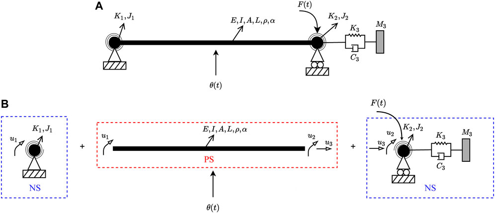
FIGURE 1. Reference structural system: (A) prototype structure and (B) its hybrid model.

Mechanical loading is supplied as a bending moment history F(t) applied to the right rotational DoF u₂, while thermal loading, applied by a heating lamp, is defined by a ramp and hold temperature history θ(t). The expressions of both read:

$F(t)=\left\{\begin{array}{c}{F}_{max}\sin \left(\frac{\pi (t-t_0)}{T}\right)\text{\hspace{0.17em},\hspace{0.17em}}{t}_0\le t\le t_0+T/2\hfill \\ 0\text{\hspace{0.17em},\hspace{0.17em}elsewhere}\hfill \end{array}\right.(16)$

$\theta (t)=\left\{\begin{array}{c}\dot{\theta }t\text{\hspace{0.17em},\hspace{0.17em}}\theta (t)<{\theta }_{max}\hfill \\ {\theta }_{max}\text{\hspace{0.17em},\hspace{0.17em}elsewhere}\hfill \end{array}\right.(17)$

where F_max and T are peak value and period of the half-side bending moment pulse applied to DoF u₂ with a time shift t₀ = 0.1 s; $\dot{\theta }=21.5$ °C/s and θ_max are temperature rate and plateau characterizing the temperature history imposed to the PS. For the sake of this example, Figure 2A depicts the bending moment history computed for F_max = 45 Nm and T = 1 s. Similarly, Figure 2B depicts the temperature history computed for θ_max = 120°C.

FIGURE 2

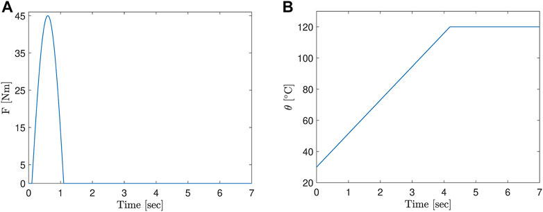
FIGURE 2. Sample time history loading: (A) bending moment history for F_max = 45 Nm and T = 1 s; (B) temperature time history for θ_max = 120°C.

Consistent with the motivations underlying the development of the GSA framework, the stiffness of the two elastic rotational springs, which play the role of boundary conditions to the PS, as well as the loading parameters, are selected as input parameters for the surrogate modeling phase. Recall that these parameters were chosen as inputs to the GSA framework, since in the majority of cases encountered in structural engineering, loading is stochastic, while the boundary conditions are highly uncertain. In line with the procedure described in Section 2, the input parameters are described by independent uniform distributions, whose bounds are summarized in Table 1.

TABLE 1

TABLE 1. Input parameters of the hybrid model.

It is important to remark that, in order to reduce the experimental effort required to validate the proposed framework, the hybrid model and loading excitation were designed such that the PS always remained in the linear response regime. As a result, HS were conducted using a single aluminum plate.

The response QoI selected for the GSA corresponds to the maximum absolute out-of-plane deflection of the tested aluminum plate, which is denoted as u_L,max.

3.2 Hybrid Simulation Setup

The 3-DoF HS test rig used to conduct HS is a stiff loading frame equipped with four electro-mechanical actuators and an infrared (IR) lamp module interfaced to an INDEL real-time computer (Abbiati et al. (2018)). The 3-DoF HS test rig is designed to test plate specimens with an approximate footprint of 200 × 500 mm and thickness varying between 1 and 3 mm. Figure 3 illustrates the architecture of the HS setup, including a close-up view of the plate specimen accommodation. Two axonometric views of the 3-DoF test rig, consisting of the main hardware components are shown in Figure 4.

FIGURE 3

FIGURE 3. Architecture of the 3-DoF HS test rig.

FIGURE 4

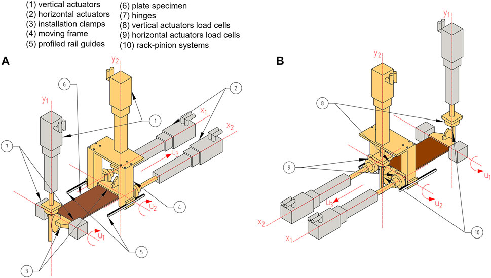
FIGURE 4. Axonometric views of the 3-DoF HS test rig with its main components (the moving parts are colored in yellow, the plate specimen is brown, while those parts fixed to the reaction frame are gray): (A) front and (B) back view perspective.

The moving parts of the test rig are colored in yellow, the plate specimen in brown and the fixed parts in gray. The latter are fixed to a reaction frame. In order to impose the u₁ and u₂ rotations, two rack-pinion systems (10) are installed along the vertical actuator y₁ and y₂ (1). The rack-pinion systems aim at transforming the commanded displacements from the actuators to rotational DoF, applied to the short edges of the plate specimen (6) through aluminum clamps (3). The two horizontal actuators x₁ and x₂ control the position of the moving frame mounted on profiled rail guides (4) and corresponding to the axial DoF u₃ of the plate specimen (6). A linear variable differential transformer (LVDT) measures the out-of-plane deflection at the mid-span of the plate specimen (labeled u_L in Figure 3). A Type K thermocouple installed at the center of the plate provides the feedback signal for the control of the IR lamp, which imposes the temperature history θ(t).

The GINLink bus connects the actuator servo-drivers INDEL stand-alone controllers (SAC4), the IR lamp and all the data acquisition (DAQ) modules to the real-time computer INDEL stand-alone master (SAM4), which executes the HS software. The latter is developed in MATLAB/SIMULINK, compiled, and downloaded to the INDEL SAM4 from the Host-PC. At each simulation time step, the HS software generates the temperature command for the IR lamp. The latter command is generated using a predefined time history temperature response (see, for example, Figure 2B). Also, at each time step of the simulation, the HS software imposes displacements u₁, u₂, and u₃ to the plate specimen, the PS. The latter displacements are computed as the response of the NS to the imposed bending moment time history response (see, for example, Figure 2A). Using force transducers the HS software reads the corresponding restoring forces r₁, r₂, and r₃, due to the imposed displacements and temperature commands, and uses them to solve the coupled equation of motion of the hybrid model. A comprehensive description of the time integration scheme used for HS is reported in Abbiati et al. (2019).

Forces were manually set to zero before starting the HS. An electric fan cools down the PS at the end of each test. Room temperature was quite stable and equal to 30°C, namely θ(0) = 30°C in Eq. 17, for the entire testing campaign.

4 Results and Discussion

The response of the hybrid model described in Section 3.1 was evaluated using the HS setup described in Section 3.2 on 200 samples of the input parameter vector generated using Latin hypercube sampling (Mckay et al. (2000)). The resulting ED X, Y was used for computing surrogate models. In a previous work of some of the authors (Abbiati et al. (2021)), 200 samples were proven to be adequate to train PCE surrogate models with acceptably small validation error. In particular, in that work, PCE estimates converged in trustworthy values with ED size larger than 50 samples. In this regard, 200 samples of the input parameter space were used in this study as well, as an initial estimate. Results presented later on demonstrate that this number of samples was sufficient to train the generalized lambda surrogate model.

Figure 5 reports out-of-plane and axial displacement histories obtained via HS for a single sample of input parameters, where u_L,max, u_3,max, u_L,0, and u_3,0 scalar quantities are highlighted. Specifically, u_L,max corresponds to the QoI (see Eq. 18) and u_3,max to the absolute maximum axial displacement while u_L,0 and u_3,0 indicate the initial position of the out-of-plane displacement and axial axes respectively, relative to the value measured during the first HS. Figure 6 describes the evolution of u_L,0 and u_3,0 scalar quantities over the entire experimental campaign.

FIGURE 5

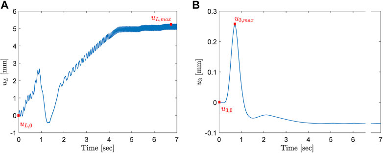
FIGURE 5. Time history response of the hybrid model with K₁ = 224.454 Nm/rad, K₂ = 118.235 Nm/rad, F_max = 48 Nm, T = 0.618 s and θ_max = 116.73°C: (A) out-of-plane displacement and (B) axial displacement.

FIGURE 6

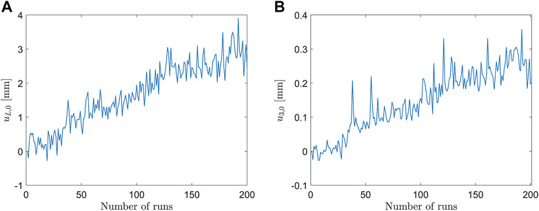
FIGURE 6. Drift in the hybrid model response: (A) u_L and (B) u₃.

4.1 Drift Observed in Measurement Data

From Figure 6 it is clear that both u_L,0 and u_3,0 quantities have a constant drift, which results in a total accumulated out-of-plane and axial displacements of 3.0 and 0.3 mm, respectively. Such a drift can be reasonably ascribed to the cumulative slippage of plate fixtures produced by heating/cooling cycles. This drift occurs regardless of the type of analysis that the HS setup was used for, and since the source of the drift is clear, it should be removed from the acquired raw data before any further post-processing. Accordingly, prior to the calculation of surrogate models, the effect of drift on u_L,max was eliminated via linear detrending with respect to u_L,0. The detrended QoI is referred to as ${\widehat{u}}_{L,max}$ and compared to original values in Figure 7. Notably, u_L,0 is independent of the parameters of the hybrid model since the initial position of the PS was set by zeroing actuator forces.

FIGURE 7

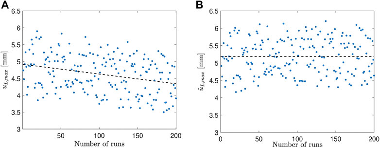
FIGURE 7. Effect of detrending on the QoI: (A) original values (u_L,max) and (B) values after detrending (${\widehat{u}}_{L,max}$). Dashed lines indicate a linear trend of data.

Consistent with the notation introduced in Section 2, surrogate modeling was performed considering the following input parameter vector and response QoI:

$\begin{array}{c}\hfill \mathit{X}=\{K_1,K_2,F_{max},T,{\theta }_{max}\}\hfill \\ \hfill \mathit{Y}=\{{\widehat{u}}_{L,max}\}\hfill \end{array}(18)$

4.2 Global Sensitivity Analysis Framework Results

A GLAM of the hybrid model dynamic response QoI was computed as explained in Section 2. In this study, we set the candidate degrees up to 5 for ${\lambda }_1^{PC}$ and 3 for ${\lambda }_2^{PC}$. In order to validate the GLAM, 10 repeated HS were performed for two validation ED points, namely 58 and 157, associated with different regions of the input parameter space and characterized by appreciably different QoI values. For each validation ED point, Figure 8 compares the GLAM prediction to the empirical distribution of the 10 related repetitions. It is observed that the GLAM correctly captures the empirical distribution of the QoI for both points. It is interesting to note that the computed GLAM model converged to zero-order polynomials for ${\lambda }_2^{PC}$, and that the two PDFs of Figure 8 are similar in shape, thus suggesting an homoscedastic stochasticity of the hybrid model, which was further verified using a PCE surrogate model. Specifically, a residual analysis was performed on the difference between the measured QoI and its PCE.

FIGURE 8

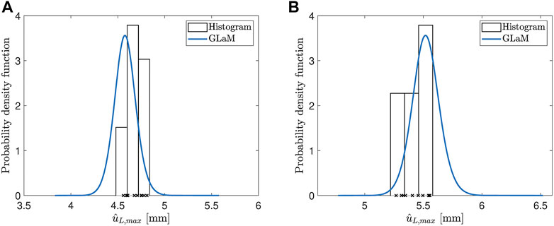
FIGURE 8. PDF of ${\widehat{u}}_{L,max}$ predicted by the GLAM versus empirical distributions for ED points: (A) 58 and (B) 157. Cross markers denote the 10 related repetitions for each point.

As highlighted by Torre et al. (2019), in presence of noisy data, PCE is a powerful denoiser, which naturally provides a surrogate of the average model response ${\mathbb{E}}_Z\left[Y|\mathit{x}\right]$. In this regard, the Tukey-Anscombe plot (Anscombe and Tukey (1963)) of Figure 9A compares the PCE output to the corresponding residual for each sample of the ED. The Q-Q plot of Figure 9B compares the empirical quantiles of the residuals normalized to unit standard deviation to the theoretical values of a standard normal distribution $\mathcal{N}(\mathrm{0,1})$. The zero-average uniform scattering of residuals highlighted by the Tukey-Anscombe plot and the fairly good agreement between empirical and theoretical quantiles highlighted by the Q-Q plot confirms that the hybrid model response was affected by a Gaussian homoscedastic additive noise.

FIGURE 9

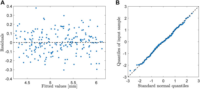
FIGURE 9. Analysis of QoI residuals with respect to PCE: (A) Tukey-Anscombe plot and (B) Q-Q plot.

As reported in Section 2.2, only first- and higher-order Sobol’ indices but not total Sobol’ indices can be obtained from the GLAM of the QoI. Instead, first and total Sobol’ indices can be computed for the QoI quantiles. Accordingly, Figure 10 provides first and total Sobol’ indices of the 5, 50 and 95% quantiles of ${\widehat{u}}_{L,max}$. The results of the GSA indicate that the temperature plateau value θ_max is the most sensitive input parameter for the selected QoI. Additionally, the equal Sobol’ indices values for each quantile unveil the homoscedastic response of the stochastic surrogate.

FIGURE 10

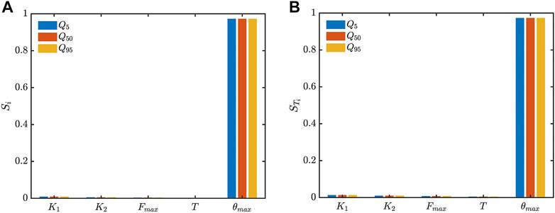
FIGURE 10. Sobol’ indices of 5, 50, and 95% quantiles of ${\widehat{u}}_{L,max}$: (A) first order and (B) total.

The development and implementation of the surrogate modeling, as well as the GSA, was performed using the UQLab software framework developed by the Chair of Risk, Safety and Uncertainty Quantification in ETH Zurich (Marelli and Sudret (2014)).

5 Conclusion

This paper described a framework for global sensitivity analysis of stochastic hybrid models. A generalized lambda surrogate modeling technique is used to compute the Sobol’ sensitivity indices for the quantiles of a response quantity of interest. The idea of using surrogate modeling to enable global sensitivity studies with few expensive-to-evaluate hybrid simulations was already presented in a previous work of the authors. However, in that work the physical substructure of the hybrid model was treated as deterministic, namely the associated aleatory uncertainties were neglected by assuming that nominally identical specimens have identical responses. Nevertheless, this assumption is still far from a realistic scenario in structural testing, as nominally identical specimens are, in practice, never actually identical. Therefore, the novelty of this work lies in the extension of global sensitivity analysis to the case of stochastic hybrid models, covering the more realistic situation where the hybrid model response for two nominally identical physical substructures is not repeatable. A great advantage of the proposed framework is that the generalized lambda surrogate model does not require repeated evaluations of the same sample. On the other hand, an assumption of the framework is that the response distribution of the stochastic hybrid model can be approximated by the generalized lambda distribution. The main limitation of the generalized lambda surrogate model is that the generalized lambda distribution is flexible but cannot represent multimodal distributions. Nevertheless, one can use a mixture of generalized lambda models to bypass this limit. In addition, a generalized lambda surrogate model can emulate the response of a stochastic model even in the case of dependent input parameters. However, for the latter case, generalized Sobol’ indices should be employed instead.

The effectiveness of the proposed framework is demonstrated in an experimental application consisting of a hybrid model with five parameters and subjected to mechanical and thermal loading. The results of the demonstration study highlight that the stochasticity of the particular hybrid model under consideration is homoscedastic with respect to the hybrid model parameters. Accordingly, both the first-order and total Sobol’ sensitivity indices of 5, 50, and 95% quantiles are almost identical. Moreover, the temperature plateau value of the thermal loading is the most sensitive parameter for the selected response quantity of interest. The outcome of the experiment demonstrates the effectiveness of the proposed global sensitivity analysis framework in revealing the inner workings of the hybrid model.

Global sensitivity analysis for stochastic hybrid models advances the current practices of hybrid simulation and establishes it as a tool capable to investigate the dynamic response of structural systems taking into account aleatory and epistemic uncertainties originating not only from numerical substructures and respective loading but also from physical specimens. The latter feature is of significant importance since the internal stochasticity of physical specimens is in general unknown and difficult to control.

Future research will address the issue of adaptive sampling of the parameter space of the stochastic hybrid model to minimize the experimental cost necessary to compute an accurate surrogate model for global sensitivity analysis.

Data Availability Statement

The raw data supporting the conclusions of this article will be made available by the authors, without undue reservation.

Author Contributions

NT: conceptualization, methodology, software, validation, writing. XZ: conceptualization, software, writing. GA: conceptualization, methodology, software, writing. SM: conceptualization, writing. BS: supervision, writing. BS: supervision, funding acquisition, writing.

Funding

This project has received funding from the European Union’s Horizon 2020 research and innovation programme under the Marie Skłodowska-Curie grant agreement No. 764547. The sole responsibility of this publication lies with the author(s). The European Union is not responsible for any use that may be made of the information contained herein. The realization of the test rig work was funded by the Swiss Secretariat of Education Research and Innovation (SERI)–Swiss Space Office (SSO) (THERMICS MdP2016 Project (Thermo-Mechanical Virtualization of Hybrid Flax/Carbon Fiber Composite for Spacecraft Structures), grant number REF-1131-61001).

Conflict of Interest

The authors declare that the research was conducted in the absence of any commercial or financial relationships that could be construed as a potential conflict of interest.

Publisher’s Note

All claims expressed in this article are solely those of the authors and do not necessarily represent those of their affiliated organizations, or those of the publisher, the editors and the reviewers. Any product that may be evaluated in this article, or claim that may be made by its manufacturer, is not guaranteed or endorsed by the publisher.

References

Abbiati, G., Covi, P., Tondini, N., Bursi, O. S., and Stojadinović, B. (2020). A Real-Time Hybrid Fire Simulation Method Based on Dynamic Relaxation and Partitioned Time Integration. J. Eng. Mech. 146, 04020104. ZSCC: NoCitationData[s0]. doi:10.1061/(asce)em.1943-7889.0001826

CrossRef Full Text | Google Scholar

Abbiati, G., Hey, V., Rion, J., and Stojadinovic, B. (2018). Thermo-Mechanical Virtualization of Hybrid Flax/Carbon Fiber Composite for Spacecraft Structures. Thermics Project, Final Report. Tech. rep., ETH Zurich.

Google Scholar

Abbiati, G., Lanese, I., Cazzador, E., Bursi, O. S., and Pavese, A. (2019). A Computational Framework for Fast-Time Hybrid Simulation Based on Partitioned Time Integration and State-Space Modeling. Struct. Control. Health Monit. 26, 1–28. doi:10.1002/stc.2419

CrossRef Full Text | Google Scholar

Abbiati, G., Marelli, S., Tsokanas, N., Sudret, B., and Stojadinović, B. (2021). A Global Sensitivity Analysis Framework for Hybrid Simulation. Mech. Syst. Signal Process. 146. doi:10.1016/j.ymssp.2020.106997

CrossRef Full Text | Google Scholar

Anscombe, F. J., and Tukey, J. W. (1963). The Examination and Analysis of Residuals. Technometrics 5, 141–160. doi:10.1080/00401706.1963.10490071

CrossRef Full Text | Google Scholar

A. Saltelli (Editor) (2008). Global Sensitivity Analysis: The Primer (Chichester, England; Hoboken, NJ: John Wiley).

Google Scholar

Bas, E. E., Moustafa, M. A., and Pekcan, G. (2020). Compact Hybrid Simulation System: Validation and Applications for Braced Frames Seismic Testing. J. Earthquake Eng. 0, 1–30. doi:10.1080/13632469.2020.1733138

CrossRef Full Text | Google Scholar

Berveiller, M., Sudret, B., and Lemaire, M. (2006). Stochastic Finite Element: a Non Intrusive Approach by Regression. Eur. J. Comput. Mech. 15, 81–92. doi:10.3166/remn.15.81-92

CrossRef Full Text | Google Scholar

Blatman, G., and Sudret, B. (2011). Adaptive Sparse Polynomial Chaos Expansion Based on Least Angle Regression. J. Comput. Phys. 230, 2345–2367. doi:10.1016/j.jcp.2010.12.021

CrossRef Full Text | Google Scholar

Browne, T. (2017). Regression Models and Sensitivity Analysis for Stochastic Simulators: Applications to Non-destructive Examination. Paris: Ph.D. thesis, Université of Paris Descartes.

Google Scholar

Chastaing, G., Gamboa, F., and Prieur, C. (2015). Generalized Sobol Sensitivity Indices for Dependent Variables: Numerical Methods. J. Stat. Comput. Simulation 85, 1306–1333. doi:10.1080/00949655.2014.960415

CrossRef Full Text | Google Scholar

Ernst, O. G., Mugler, A., Starkloff, H.-J., and Ullmann, E. (2012). On the Convergence of Generalized Polynomial Chaos Expansions. Esaim: M2an 46, 317–339. doi:10.1051/m2an/2011045

CrossRef Full Text | Google Scholar

Freimer, M., Kollia, G., Mudholkar, G. S., and Lin, C. T. (1988). A Study of the Generalized Tukey Lambda Family. Commun. Stat. - Theor. Methods 17, 3547–3567. doi:10.1080/03610928808829820

CrossRef Full Text | Google Scholar

Idinyang, S., Franza, A., Heron, C. M., and Marshall, A. M. (2019). Real-time Data Coupling for Hybrid Testing in a Geotechnical Centrifuge. Int. J. Phys. Model. Geotechnics 19, 208–220. doi:10.1680/jphmg.17.00063

CrossRef Full Text | Google Scholar

Iooss, B., and Ribatet, M. (2009). Global Sensitivity Analysis of Computer Models with Functional Inputs. Reliability Eng. Syst. Saf. 94, 1194–1204. doi:10.1016/j.ress.2008.09.010

CrossRef Full Text | Google Scholar

Karian, Z. A., and Dudewicz, E. J. (2000). Fitting Statistical Distributions: The Generalized Lambda Distribution and Generalized Bootstrap Methods. New York: Chapman and Hall/CRC Press.

Google Scholar

Marelli, S., Lamas, C., Konakli, K., Mylonas, C., Wiederkehr, P., and Sudret, B. (2019). “UQLab User Manual – Sensitivity Analysis,” in Tech. Rep. # UQLab-V1.3-106, Chair of Risk, Safety and Uncertainty Quantification (Switzerland: ETH Zurich).

Google Scholar

Marelli, S., and Sudret, B. (2014). “UQLab: A Framework for Uncertainty Quantification in Matlab,” in Proc. 2nd Int. Conf. on Vulnerability, Risk Analysis and Management (ICVRAM2014), Liverpool, United Kingdom, 2554–2563. doi:10.1061/9780784413609.257

CrossRef Full Text | Google Scholar

Mckay, M. D., Beckman, R. J., and Conover, W. J. (2000). A Comparison of Three Methods for Selecting Values of Input Variables in the Analysis of Output from a Computer Code. Technometrics 42, 55–61. doi:10.1080/00401706.2000.10485979

CrossRef Full Text | Google Scholar

Moustafa, M., and Mosalam, K. (2015). “Development of Hybrid Simulation System for Multi-Degree- of-Freedom Large-Scale Testing,” in 6th International Conference on Advances in Experimental Structural Engineering, Urbana-Champaign, United States (): University of Illinois).

Google Scholar

Rasmussen, C. E., and Williams, C. K. I. (2006). Gaussian Processes for Machine Learning. Adaptive Computation and Machine Learning. Cambridge, Mass: MIT Press.

Google Scholar

Sauder, T., Marelli, S., Larsen, K., and Sørensen, A. J. (2018). Active Truncation of Slender marine Structures: Influence of the Control System on Fidelity. Appl. Ocean Res. 74, 154–169. doi:10.1016/j.apor.2018.02.023

CrossRef Full Text | Google Scholar

Schellenberg, A. H., Mahin, S. A., and Fenves, G. L. (2009). “Advanced Implementation of Hybrid Simulation,” in Tech. Rep. PEER 2009/104, Pacific Earthquake Engineering Research Center (Berkeley: University of California).

Google Scholar

Sobol’, I. M. (1993). Sensitivity Estimates for Nonlinear Mathematical Models. Math. Model. Comp. Exp. 1, 407–414.

Google Scholar

Sudret, B. (2008). Global Sensitivity Analysis Using Polynomial Chaos Expansions. Reliability Eng. Syst. Saf. 93, 964–979. doi:10.1016/j.ress.2007.04.002

CrossRef Full Text | Google Scholar

Torre, E., Marelli, S., Embrechts, P., and Sudret, B. (2019). Data-driven Polynomial Chaos Expansion for Machine Learning Regression. J. Comput. Phys. 388, 601–623. doi:10.1016/j.jcp.2019.03.039

CrossRef Full Text | Google Scholar

Vilsen, S. A., Sauder, T., Sørensen, A. J., and Føre, M. (2019). Method for Real-Time Hybrid Model Testing of Ocean Structures: Case Study on Horizontal Mooring Systems. Ocean Eng. 172, 46–58. doi:10.1016/j.oceaneng.2018.10.042

CrossRef Full Text | Google Scholar

Xiu, D., and Karniadakis, G. E. (2002). The Wiener--Askey Polynomial Chaos for Stochastic Differential Equations. SIAM J. Sci. Comput. 24 (2), 619–644. doi:10.1137/S1064827501387826

CrossRef Full Text | Google Scholar

Zhu, X., and Sudret, B. (2021a). Emulation of Stochastic Simulators Using Generalized Lambda Models. Siam/asa J. Uncertainty Quantification 9, 1345–1380. doi:10.1137/20m1337302

CrossRef Full Text | Google Scholar

Zhu, X., and Sudret, B. (2021b). Global Sensitivity Analysis for Stochastic Simulators Based on Generalized Lambda Surrogate Models. Reliability Eng. Syst. Saf. 10. doi:10.1016/j.ress.2021.107815

CrossRef Full Text | Google Scholar

Zhu, X., and Sudret, B. (2020). Replication-based Emulation of the Response Distribution of Stochastic Simulators Using Generalized Lambda Distributions. Int. J. Uncertaintyquantification 10, 249–275. doi:10.1615/int.j.uncertaintyquantification.2020033029

CrossRef Full Text | Google Scholar