Analysis of the Duration of High Winds During Landfalling Hurricanes

The duration of wind storms over a threshold wind speed value is known to be an important parameter in determining damage and losses, with losses tending to increase with the duration. This is because peak pressures tend to increase with longer duration, many building components and cladding systems are vulnerable to different types of fatigue mechanisms, and the yielding of linear elastic materials in the plastic range depends on the number of load cycles. A hurricane model was used to examine the duration of high winds in the United States at Miami, Galveston, and Charleston with the goal of establishing duration statistics for hurricanes as a function of peak wind speed. It was found that the duration of high winds, defined as the time that the 10 min wind speeds are within 30% of the peak 10 min wind speed, had a significant variation with a range from tens of minutes to more than 20 h, depending on location. The median duration ranged from 1.5 to 4 h at the three locations, depending on location and the design wind speed level (i.e., the risk Category of the building). These results were used to establish a simple normalized model for wind speed as a function of time, which could be used together with the design wind speed to establish load cycles for design.

Introduction

The duration of storms, which is determined by the combination of the storm size and translation speed, is known to be an important parameter in determining damage and losses, for several reasons. First, the statistics for gust wind speeds and peak aerodynamic (i.e., pressure) loads yield larger magnitudes with longer durations, all else being equal (Cook and Mayne, 1979). Second, many building components are susceptible to fatigue issues such as metal roof decks with fixed, pierced fasteners (e.g., screws), which are susceptible to low cycle fatigue (Mahendran, 1995; Xu, 1995; Kumar and Stathopoulos, 1998), and glazing and windows, which are susceptible to static fatigue (Charles, 1958; Minor, 1981). Many components also have significant non-linear yield characteristics. One example is nailed connections used in wood-frame construction, that can be modeled as bi-linear with extensive yielding (i.e., pull-out), which is strongly dependent on the number of peak pressure cycles for complete withdrawal (Morrison and Kopp, 2011) and, therefore, on the storm duration (Guha and Kopp, 2014). Third, rainwater penetration contributes significantly to losses (Sparks et al., 1994; Standohar-Alfano et al., 2017).

Loss models such as HAZUS (Vickery et al., 2006) indirectly account for storm duration by modeling the passage of storms through a region and, in particular, the probability of failure in each segment of time (e.g., each 10 min interval). In contrast, most design for wind effects considers the duration of strong winds to be 1 h (Cook and Mayne, 1979; Kopp and Morrison, 2018), which appears to be related to the concept of the spectral gap. The spectral gap is a point in the wind speed spectrum with low energy levels that separates the wavelengths with high energy due to microscale turbulence from those due to synoptic-scale and mesoscale fluctuations. Wind speed fluctuations below an hour are assumed to be stochastic and dependent on terrain roughness, i.e., these fluctuations are turbulence, due to the spectral gap. Boundary layer wind tunnel testing is based on this assumption. In contrast, tornadoes and, more generally, thunderstorms, tend to have much shorter durations of high winds at any particular location. Tropical cyclones, such as hurricanes, are much larger scale and measurements have shown that they could be considered to be statistically stationary over tens of minutes (Masters et al., 2010). However, tropical cyclones do have considerable variation in size and translation speed, and, therefore, duration, which has not generally been considered in design.

One situation where duration has been explicitly considered was for the development of the “low-high-low” test standard for low cycle fatigue (Jancauskas et al., 1994; Mahendran, 1995). This was a result of the devastation caused by Tropical Cyclone (TC) Tracy, where the failure of metal roof decking, caused by low cycle fatigue, was ubiquitous. As a result, a new test standard for such roof cladding was developed based on the concept of the design cyclone. Jancauskas et al. (1994) based the design cyclone on the wind speed time history observed for TC Tracy and other destructive tropical cyclones, which had an estimated maximum, 15 min mean wind speed of 42 m/s (Henderson et al., 2009) and wind speeds within 30% of this maximum over a 5 h duration. The change in wind direction over this period was about 100°. Details of their approach can also be found in Kopp et al. (2012).

The objective of this study is to examine the variation of duration for hurricanes near their design wind speeds. The approach will be to use the hurricane model of Li and Hong (2014) with a particular focus on three locations, viz., Miami-Dade (FL), Galveston (TX), and Charleston (NC). This analysis will inform an assessment of design cyclones considering the statistical variations of duration and wind speed, but also allow the assessment of appropriate durations for peak pressures and for load cycles. These three locations were chosen to represent three distinct locations along the Atlantic and Gulf Coasts in order to get a sense of the variability of these effects.

Methodology

Data Set for Hurricane Wind Speeds and Duration

The numerical model employed in this study is the same as that developed in Li and Hong (2014), which includes both a wind field model and a full track model. The calculated wind fields using this model compare favourably to the reconstructed wind field from H*Wind (Powell et al., 1998). The HURDAT/HURDAT2 best-track dataset (Landsea and Franklin. 2013) was used to develop the track model, the performance of which was validated by comparing the statistics of the key hurricane parameters calculated from simulated tracks to those from the HURDAT dataset. In addition, Li and Hong (2014) concluded that the estimated return period hurricane wind speed contour maps based on the developed track model, adopted wind field model and equations for defining the wind field parameters result in the comparable wind hazard contour maps to those given in Vickery et al. (2009a). The functional form of the empirical track model is essentially the same as that in Vickery et al. (2000), and similar to that in Vickery et al. (2009a). By using the full track model, storm tracks originating in the North Atlantic basin are simulated from genesis to lysis.

Each simulated track contains the basic information, consisting of latitude and longitude of the storm, heading, translation velocity, and central pressure difference of the storm. These key parameters are obtained for each 6 h time interval and are then linearly interpolated to every 15 min. The information from the interpolated tracks is then used to calculate the wind speed at the particular sites. To simplify the calculation for the 100,000 years of hurricanes activities, and since we are interested primarily in design-level events, only those storms within a radius of 250 km from the site are considered. Parameters defining the wind field, such as the radius to the maximum wind speed (R_max) and the Holland parameter B are calculated from the formulas found in the literature (Vickery et al., 2009a; Vickery et al., 2009b). The final samples of the wind speed duration are 10 min mean wind speeds at the height of 10 m. Figure 1 provides results from Li and Hong (2014), which shows the tracks in the Atlantic basin and the 700 years wind speeds on the Gulf and Atlantic coasts of the United States A comparison of the estimated design level wind speeds based on this model and those recommended in ASCE 7–16 will be presented in Analysis of Conditional Duration Statistics.

FIGURE 1

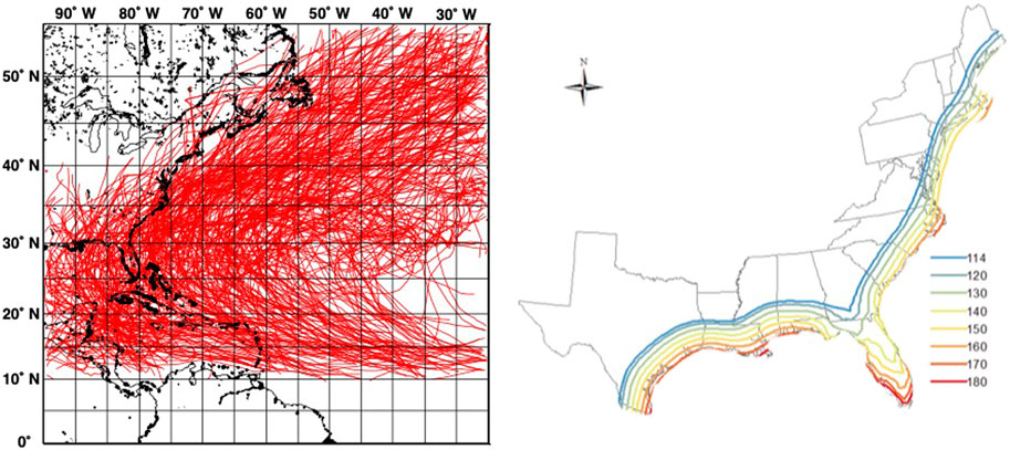
FIGURE 1. Results of the hurricane model showing tracks in the Atlantic basin (left) and the 700-yr design wind speed (mph) contours (right) from the data of Li and Hong (2014).

Definition of the Hurricane Time History Parameters

In this section, the hurricane wind speed at particular sites is developed and presented as a normalized or standardized function of time. Two typical cases of the wind speed time history are considered: 1) when the eyewall passes over a site, leading to a double peak in the wind speed time history at that site, and 2) when the eyewall misses the site, leading to a wind speed time history with a single peak. In other words, a single peak is formed when the closest distance from the center of the storm to the site is greater than R_max; if the distance is less than R_max, two peaks are formed. Examples of data from the simulation are shown in Figure 2. Samples of wind speed duration are obtained from the simulation results for 10 min mean wind speeds greater than a minimum threshold wind speed, V_min = 18 m/s, which is close to 70% of the lowest value of sustained (1 min mean) wind speed for Category I hurricanes (118 km/h), as defined by the National Hurricane Center. The rationale for the 70% value is discussed below.

FIGURE 2

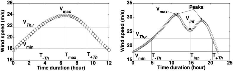
FIGURE 2. Typical wind speed duration of the simulated storm passing by specific site with single peak (left) and double peak (right).

The lowest wind speed that is of interest in terms of applying a damaging wind load to the structure is defined as the threshold wind speed, V_T,r. This can be expressed in terms of the proportion of the maximum storm wind speed, V_max, by,

$r=\frac{V_{T,r}}{V_{\max }},(1)$

where r is the ratio of the threshold to maximum wind speed. The choice for the ratio, r, is discussed further below and in reference to Figure 2.

For the double-peak case, the minimum speed between the two peaks is denoted as V_int. The times corresponding to the threshold wind speeds to the left (i.e., earlier) and right (i.e., later) side of the peak wind speed, V_max, are denoted as T_−Th and T_+Th, respectively. The time corresponding to V_max and V_int are denoted as, T_max and T_int, respectively.

In order to develop a statistically based design cyclone, the wind speed time history is normalized, considering both the maximum wind speed and the duration. For the single peak case, the wind speeds are normalized by the maximum wind speed, V_max, such that,

$V_s=\frac{V}{V_{max}}.(2)$

At the threshold wind speed, V_T,r, the normalized speed, V_s = r. The time duration is normalized according to the following equation, such that the normalized time, T_s = ±1 when V_s = r, i.e.,

$T_s=\frac{T-T_{max}}{\left|T_{max}-T_{\pm Th}\right|}.(3)$

It should be noted that, since the durations on either side of the maximum wind speed can differ, the normalizations on either side of the maximum are different. The effective total duration of the hurricane, T_tot, occurs over the time that V_s ≥ V_min/V_max.

For the double-peak cases, additional considerations are required. For simplicity in practical situations (such as the development of cycle counts and loads for a low-cycle fatigue test standard), it is useful to map the double-peak cases as equivalent single peak cases. If the V_int (defined in Figure 2) of a double-peak case is lower than threshold wind speed, the double-peak case is divided into two single peak cases. For double-peak cases for which V_int is greater than the threshold wind speed, to obtain the total duration of the event, T_tot, above the minimum wind speed, V_min, the velocity and time can be normalized using Eq. 2 and Eq. 3 provided V_s ≥ V_min/V_max and the T_Th values are obtained for the extreme time values when V_s = r. To obtain the duration of time when V_s ≥ r, the interval of time when V_s ≤ r is removed, as is the case when the statistics of T_Th are considered in the next section.

The threshold wind speed value also needs discussion. In the design cyclone of Jancauskas et al. (1994), r = 0.7. This yields a wind load that is nominally about half the maximum. It was reported by Gavanski et al. (2016), from an analysis of wind tunnel records, that the range from the lower to the upper bounds of the extreme values of pressure coefficient, Cp, for durations of 10 min, i.e., the ratio of the range of peak pressure coefficients associated with 10 min mean wind speeds is about 0.5. Given this possibility, the reasonable range of wind speeds to consider for the peak loads is over the duration when V_s > ∼0.7. This range would also be appropriate for glazing and glass since static fatigue under wind load is controlled by the peak pressures (Gavanski and Kopp, 2011).

Results

Analysis of Effective Total Durations of Hurricanes

To study the effective total duration of the hurricane wind speeds, the design wind speeds for the ASCE seven Risk Category II for three stations, Miami, Galveston, and Charleston, are used as baseline reference wind speeds. The design wind speeds for Risk Category II buildings based ASCE 7–16 are 3 s gust wind speeds of 75 m/s (168 mph) for Miami, 67 m/s (150 mph) for Galveston, and 65 m/s (146 mph) for Charleston. These correspond to 10 min mean wind speed of 51 m/s for Miami, 46 m/s for Galveston and, 45 m/s for Charleston. For the conversion, a factor of 1.47, calculated based on ESDU (Vickery et al., 2006) is used to convert 3 s gust wind speed to 10 min mean wind speed.

There are four target wind speeds that are selected as V_T,r values. They are wind speeds within 5, 10, 20, and 30% of the design wind speeds for each station. In other words, given the design wind speed, the wind speeds considered in this exercise must be greater than 95, 90, 80 and 70% of the design (peak) wind speed, respectively. Consequently, four threshold 10 min mean wind speeds selected for Miami are 49, 46, 41, and 36 m/s, respectively; for Galveston are 43, 41, 37, and 32 m/s, respectively; and for Charleston are 43, 40, 36, and 31 m/s, respectively. The distribution of the time duration for each of these is shown in Figure 3, along with a fit using the GEV distribution. Four different probabilistic distributions, namely the Lognormal distribution, Gamma distribution, Weibull distribution and Generalized extreme value (GEV) distributions, were fit to the empirical Cumulative Distribution Functions (CDF) in Figure 3. In general, the GEV distribution provides the better fit, based on the AIC criterion (Akaike, 1974).

FIGURE 3

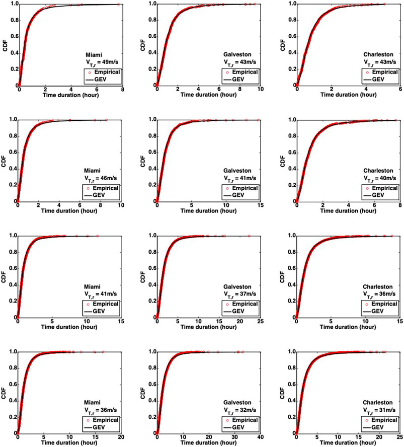
FIGURE 3. Time duration of wind speeds above the threshold speed.

Figure 3 presents the CDFs for the three locations for the range of threshold wind speeds. Several observations can be made. First, the effective duration ranges from close to zero (i.e., a single 10-min segment) to over 30 hours, depending on the location and threshold speed. Clearly, as the threshold wind speed decreases, the duration increases. Interestingly, the duration of winds for a threshold of 95% of the design speed can be up to 8 hours. However, median values are typically about 2 hours or less for the thresholds examined, while 80th percentile values for the 70% threshold speed are in the range of 2 to 3 hours at the three locations. The threshold wind speed equal to 70% of the design wind speed is the primary focus of the remainder of the analysis in order to develop a statistical basis for cyclone design consideration, based on the rationale provided earlier.

For the development of the statistically based design cyclone, the symmetry of duration about the maximum speeds is investigated to see if there is a bias to one side or the other. The relation of the total time duration is defined as ΔT = T_+Th−T_−Th, while the time duration prior to the maximum wind speed is defined as ΔT_L = T_max−T_−Th. The relationship of these two terms is investigated for each of three stations by adopting the 70% of the design wind speed as the threshold speed (i.e., V_s = 0.7). Using a lower cutoff threshold wind speed of 30 m/s, the correlation coefficient of ΔT_L and ΔT is about 0.92 for Miami, 0.93 for Galveston, and 0.94 for Charleston. This indicates that ΔT and ΔT_L may be adequately described by a linear relationship. The best linear fit between ΔT and ΔT_L for each of three stations is shown in Figure 4, where the coefficient of determination (R²) for each fit is greater than 0.85, indicating that the linear model performs adequately. The slope of these linear models ranges from 1.87 to 1.97, which is close to 2.0. For both simplicity and practicality, $T_{max}=\Delta T/2$ could be used since, by adopting such an approximation, the mean wind time history becomes symmetric with respect to $T_{max}$. With this, the modeling of the duration of high winds becomes the assignment of a preferred probability distribution model for ΔT and finding the distribution parameters.

FIGURE 4

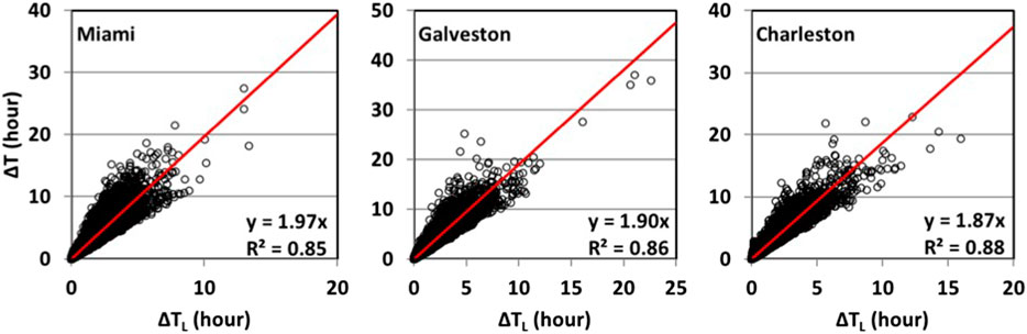
FIGURE 4. Relation of ΔT_L and ΔT for three stations.

Analysis of Normalized Hurricane Wind Speed Versus Duration Curve

As discussed previously, the double peak samples can be reasonably converted into an equivalent single peak sample. The time duration of a single peak wind speed time series can then be normalized by using Eqs. 2, 3. The threshold wind speed of 0.7V_max is used (which results in all samples being greater than 30 m/s. The normalized storm passages can then be fit into one curve. It was found that a fourth-order polynomial could be used to represent $V_s\left(T_s\right)$ adequately, provided that three constraints are applied. This results in:

$V_s\left(T_s\right)=a_0+a_1{T}_s+a_2{T}_s^2+a_3{T}_s^3+a_4{T}_s^4,(4)$

where a_i are the parameters estimated via fitting using the least-square method. The three constraints for Eq. 4 are V_s (0) = 1, V_s (−1) = 0.7 and V_s (1) = 0.7. The first constraint results in a₀ = 1. The summation of the latter two constraints results in a₂ + a₄ = −0.3. The subtraction of the latter two constraints results in a₁ = −a₃. This reduces the number of variables in Eq. 5 to two, which can be re-expressed as,

$V_s\left(T_s\right)=1+a_1{T}_s+a_2{T}_s^2-a_1{T}_s^3-\left(0.3+a_2\right)T_s^4.(5)$

The normalized samples for three stations are fit into Eq. 5. The samples, as well as, the fitted curve are plotted in Figure 5. The R² value for the fit is about 0.97, which indicates the fourth-order polynomial formula is a reasonable model. In Figure 5, the estimated value a₁ = 0.0038, and a₂ = −0.46, which indicates that, on average, the normalized duration can be approximated by a quadratic formula. However, Figure 5 also indicates that there are some relatively large variations of the normalized hurricane wind speed duration, as can be seen in the relatively wide band of the normalized curve. To study the uncertainty in a₁ and a₂, each curve based on a sample hurricane is fit to Eq. 5, following which, the samples of a₁ and a₂ are fit into several probabilistic models, including the Logistic distribution, Normal distribution, GEV distribution, and Gumbel distribution. Based on AIC criterion, it was found that the Logistic distribution fit the samples the best. The Logistic distribution can be expressed as,

$f\left(a_i;\mu ,s\right)=e^{\frac{a_i-\mu }{s}}/\left(s{\left(1+e^{\frac{a_i-\mu }{s}}\right)}^2\right),(6)$

where $a_i$ is the random variable, µ and s are distribution parameters that are estimated by using the maximum likelihood method in the present study. The histogram of the obtained values of a₁, a₂, and the fitted PDFs are shown in Figure 6, illustrating the adequacy of the Logistic distribution fit. Plots of the value of a₁, a₂, and its corresponding maximum wind speed of the storm are also presented in Figure 6 for each sampled hurricane. The R² and correlation coefficients shown in the plots indicate that the coefficient, a₁, a₂, and maximum wind speed of the storm could be assumed to be uncorrelated. It should be noted that the number of available samples of a_i decreases as the maximum wind speed of the cyclone increases.

FIGURE 5

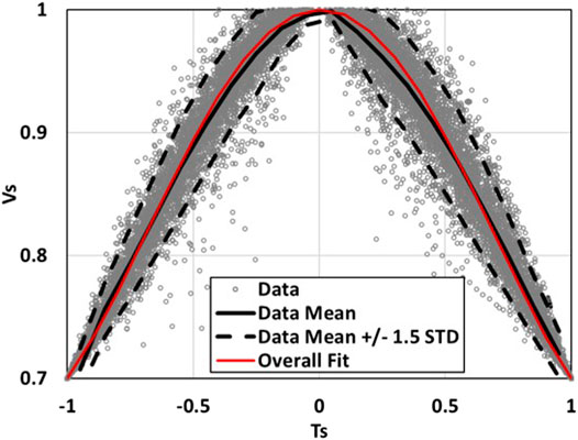
FIGURE 5. Fitted normalized hurricane wind duration for three stations.

FIGURE 6

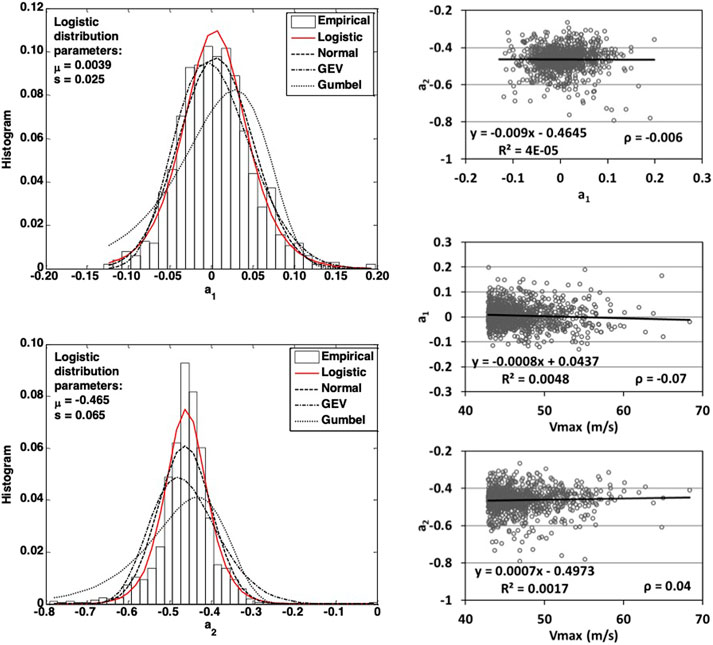
FIGURE 6. PDF of coefficient a1, a2 and relation of a1, a2, and the corresponding peak wind speeds.

Analysis of Conditional Duration Statistics

Design wind speeds from ASCE 7–16 for different risk categories for the three selected locations are listed in Table 1, where the design wind speeds are given in terms of the 3 s gust wind speed (in mph). The predicted 700 years return period values of the hurricane wind speeds by using the model in Li and Hong (2014) are also listed in Table 1. In general, the difference between the estimated 700 years return period values of the hurricane wind speed is within about 3% of the design wind speed in ASCE 7–16 for these three stations based on 100,000 years of simulated hurricanes. This implies that the simulated hurricane wind time series are comparable statistically to those used to derive the design wind speeds for ASCE 7–16.

TABLE 1

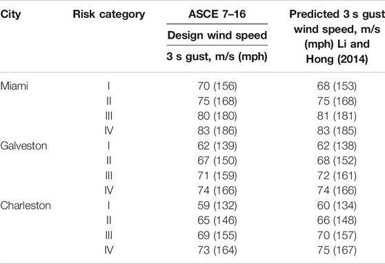
TABLE 1. Design wind speeds for Miami, Galveston, and Charleston.

For the statistical analysis of the effective wind duration for a₁ and a₂, given a specified maximum wind speed, it is assumed that the samples from each of the simulated hurricanes with the maximum wind speed within +/− 1 m/s of the specified maximum wind speed can be grouped together. For example, samples of the wind duration for peak wind speed within 50 m/s and 52 m/s can be grouped to represent the samples for a specified wind speed of 51 m/s.

For the probabilistic analysis of the wind duration, three specified wind speeds are selected for each of the considered cities to cover the design wind speed for the different risk categories. The samples of wind duration are fit into four different probabilistic distributions, namely the Lognormal, Gamma, Weibull, and GEV distributions. Based on AIC criterion and the maximum likelihood method, the preferred distribution is the GEV distribution. The empirical cumulative probabilistic distribution and fitted GEV distribution are presented Figure 7.

FIGURE 7

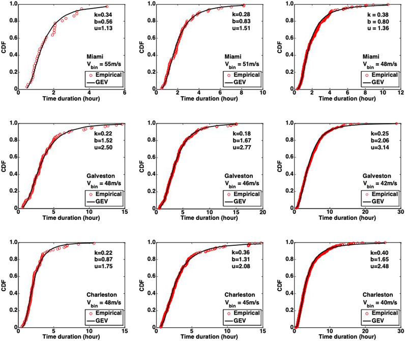
FIGURE 7. Empirical distribution and fitted probabilistic distribution for wind duration in each peak wind speed bin for each city.

Practically, for the purposes of developing a design cyclone, one may be more interested in the average storm duration, given the maximum wind speed of a storm. For this purpose, the percentiles of the duration of different maximum storm wind speeds are presented in Figure 8. An exponential model is used to fit the 50-percentile of the duration for each of the three stations. It can be seen from the R² values provided in the figure that the exponential model fits the data well. Considering the range of design wind speeds from Category I to IV, the median values of the duration are about 1.5–2 h for Miami, 2.5–4 h for Galveston, and 2–3 h for Charleston. The 80th percentile of the duration ranges from two to 3.5 h for Miami, 5–7 h for Galveston, and 3–5 h for Charleston. Such long-duration storms would tend to be more destructive for fatigue sensitive structures and structural components due to the greater number of load cycles and the greater likelihood of larger peak pressures.

FIGURE 8

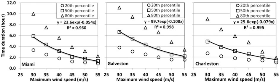
FIGURE 8. Time durations conditional on maximum hurricane wind speeds for three stations.

Discussion

Based on the statistical analysis of hurricane passage data at the three locations, Eq. 5 provides a model of the normalized wind speed time history for the design cyclone, which can be made dimensional using the design wind speed, such as those from ASCE 7–16 in Table 1, with the duration from Figure 8. Although the methodology developed in the study could be applied to other sites, here, we discuss how the durations of high winds for these design-level hurricanes may affect existing design provisions for the peak loads and for building systems that depend on the load cycles.

The typical duration of high winds for establishing peak pressures is 1 h (e.g., Cook and Mayne, 1979; Gavanski et al., 2016; Li et al., 2020). Cook and Mayne (1979) showed that the effects of duration for peak pressure coefficients that follow the Gumbel distribution is proportional to ln(T/t), where the cumulative distribution function for the Gumbel distribution is

$F_g\left(Cp\right)=exp\left\{-exp\left[-\alpha \left(Cp-U\right)\right]\right\},(7)$

and α and U are shape parameters that depend on the observed peak values. The changes of distribution parameters due to the change in duration are estimated via conversion of the shape parameters such that

${\alpha }_T={\alpha }_t,(8)$

$U_T=U_t+ln\left(T/t\right)/{\alpha }_t,(9)$

where T and t are the new and original durations. The design cyclone represented by Eq. 5 indicates that the proportion of time that the 10-min wind speed is within 5% of the maximum is about 41% of the total duration. Using the median durations from Figure 8 and the Category one design wind speeds in Table 1 indicate that the average duration from the three sites is about 3 h, which leads to durations of wind speeds within 5% of the maximum of about 1.2 h. This is close to the usual design duration of t = 60 min. Thus, using this average indicates that the design values do not need to change, although the variation across regions implies regionally dependent risk. In contrast, hurricanes of longer duration such as those of the 80th percentile duration in Figure 8, indicate that the average duration across the three sites for the Category I design wind speed increases to just above 5 h, or a 70% increase in duration. Gavanski et al. (2016) and Li et al. (2020), who were examining the effects of sampling duration and data handling on the estimates of peak pressure coefficients from wind tunnel data for low-rise buildings and mid-range high-rise buildings, respectively, provide some indication as to how changes in duration affect the peak coefficients. The data presented by these authors indicate that a doubling of the duration increases the peak coefficients in the range of about 10%, which is also roughly the measurement uncertainty for wind tunnel pressure coefficients.

For cyclic loads, the design cyclone can be combined with aerodynamic time series data for the class of building or cladding system under consideration to obtain the load amplitudes and cycle counts, as done by Henderson et al. (2009) for low-cycle fatigue of screw-fastened metal roof decking and Gavanski and Kopp (2011) for glazing. Both of these considered 5 hour-long design cyclones in their analyses. The current data indicates that a 5 h duration is consistent with approximately an 80th percentile duration for Category I buildings (when averaged across the three locations). For higher Category buildings, or for the median durations, the durations are shorter so that the cycle counts compared to a 5 h duration would be reduced proportionately and test or design standards based on 5 h may be viewed as conservative. However, for glazing, the detailed conclusions of Gavanski and Kopp (2011) are worth reviewing since they did find some issues with the choice of the probabilities associated with peak pressures as they relate to glazing design and failures under static fatigue. In particular, these authors recommended that, for glazing, the probability of non-exceedance of the pressure coefficients should be 90th-percentile hourly peaks, rather than median or even 78th-percentile peaks. This can be understood by considering Brown’s integral (Brown, 1974; Minor, 1981), whereby the equivalent peak pressure for a prescribed loading duration, t_ref, is represented by

$p_{eq}\left(t_{ref}\right)={\left[\underset{0}{\overset{T}{{\displaystyle \int }}}{p}^s\left(t\right)dt/t_{ref}\right]}^{1/s},(10)$

where p_eq is the equivalent pressure for t_ref = 3 s, the equivalent static loading duration, T = 5 h is the storm duration, p(t) is the pressure time history on the glazing element over the duration of the storm, and s is an exponent related to the damage accumulation mechanism, which is typically in the range of 10–15 (e.g., Gavanski and Kopp, 2011, used s = 13). The damage accumulation model, when considering the nature of fluctuating wind loads, can be viewed as a summing up of the effects of all of the large peak pressures into an equivalent static load (p_eq) for the equivalent duration (t_ref). While ASCE seven is silent on the interpretation of the peak pressures for glazing design, it is generally assumed to be that p_eq is the wind-induced pressure as set out in the standard, which is formed from an instantaneous pressure coefficient referenced to a 3 s long peak gust speed, and that all of the peaks occurring in the storm should add up to an equivalent static duration, t_ref = 3 s, that is the same as the gust speed duration. The shorter durations found in Figure 8, presuming median storm durations are used for design, indicate that the 90th-percentile peak may not be required and the 78th-percentile hourly peak recommended by Cook and Mayne (1979) and used by Kopp and Morrison (2018) is adequate.

Conclusions

A hurricane model was used to examine the statistics of the duration of high winds at the three locations (Miami, Galveston, Charleston) with the goal of developing a model for design hurricanes. First, it was found that a simple polynomial function could be used to represent the normalized wind speed vs. time relationship, with normalizing parameters of the maximum 10 min wind speed during the passage of the hurricane and the total time duration that the wind speed was above a threshold value. For hurricanes where the eyewall passed over the location leading to a double peak in the wind speed, combining the two parts into the simple polynomial function with a single peak was sufficiently accurate. Second, the duration of high winds, with 10 min wind speeds within 30% of the peak 10 min wind speed, had a significant variation with a range from tens of minutes to more than 20 h, depending on location, for peak wind speeds in the design-level range. Median total durations for peak storm wind speeds similar to or greater than the corresponding 300 years return period design wind speeds ranged from 1.5 to 4 h, depending on location and the risk Category of the building.

Data Availability Statement

The raw data supporting the conclusions of this article will be made available by the authors, without undue reservation.

Author Contributions

All authors contributed to the data analysis and writing of the manuscript. SHL and HH developed the hurricane model.

Funding

This work was funded by the Natural Sciences and Engineering Research Council (NSERC) of Canada under the Collaborative Research and Development program, with support from the Institute for Catastrophic Loss Reduction (ICLR).

Conflict of Interest

The authors declare that the research was conducted in the absence of any commercial or financial relationships that could be construed as a potential conflict of interest.

References

Akaike, H. (1974). A New Look at the Statistical Model Identification. IEEE Trans. Automat. Contr. 19 (6), 716–723. doi:10.1109/tac.1974.1100705

CrossRef Full Text | Google Scholar

Brown, W. G. (1974). A Practicable Formulation for the Strength of Glass and its Special Application to Large platesPub. No. NRC 14372. Ottawa, Canada: National Research Council.

Charles, R. J. (1958). Static Fatigue of Glass. I. J. Appl. Phys. 29 (11), 1549–1553. doi:10.1063/1.1722991

CrossRef Full Text | Google Scholar

Cook, N. J., and Mayne, J. R. (1979). A Novel Working Approach to the Assessment of Wind Loads for Equivalent Static Design. J. Wind Eng. Ind. Aerodyn. 4 (2), 149–164. doi:10.1016/0167-6105(79)90043-6

CrossRef Full Text | Google Scholar

Gavanski, E., and Kopp, G. A. (2011). Storm and Gust Duration Effects on Design Wind Loads for Glass. J. Struct. Eng. 137 (12), 1603–1610. doi:10.1061/(asce)st.1943-541x.0000397

CrossRef Full Text | Google Scholar

Gavanski, E., Gurley, K. R., and Kopp, G. A. (2016). Uncertainties in the Estimation of Local Peak Pressures on Low-Rise Buildings by Gumbel-Fitting Approach. J. Struct. Eng. 142 (11), 100001556–100011061. doi:10.1061/(asce)st.1943-541x.0001556

CrossRef Full Text | Google Scholar

Guha, T. K., and Kopp, G. A. (2014). Storm Duration Effects on Roof-To-Wall-Connection Failures of a Residential, Wood-Frame, Gable Roof. J. Wind Eng. Ind. Aerodyn. 133, 101–109. doi:10.1016/j.jweia.2014.08.005

CrossRef Full Text | Google Scholar

Jancauskas, E. D., Mahendran, M., and Walker, G. R. (1994). Computer Simulation of the Fatigue Behaviour of Roof Cladding during the Passage of a Tropical Cyclone. J. Wind Eng. Ind. Aerodyn. 51, 215–227. doi:10.1016/0167-6105(94)90005-1

CrossRef Full Text | Google Scholar

Kopp, G. A., and Morrison, M. J. (2018). Component and Cladding Wind Loads for Low-Slope Roofs on Low-Rise Buildings. J. Struct. Eng. 144 (4), 04018019. doi:10.1061/10.1061/(asce)st.1943-541x.0001989

CrossRef Full Text | Google Scholar

Kopp, G. A., Morrison, M. J., and Henderson, D. J. (2012). Full-scale Testing of Low-Rise, Residential Buildings with Realistic Wind Loads. J. Wind Eng. Ind. Aerodyn. 104-106, 25–39. doi:10.1016/j.jweia.2012.01.004

CrossRef Full Text | Google Scholar

Kumar, K. S., and Stathopoulos, T. (1998). Fatigue Analysis of Roof Cladding under Simulated Wind Loading. J. Wind Eng. Ind. Aerodyn. 77–78, 171–183.

Google Scholar

Landsea, C. W., and Franklin, J. L. (2013). Atlantic Hurricane Database Uncertainty and Presentation of a New Database Format. Mon. Wea. Rev. 141, 3576–3592. doi:10.1175/mwr-d-12-00254.1

CrossRef Full Text | Google Scholar

Li, S. H., and Hong, H. P. (2014). Observations on a Hurricane Wind Hazard Model Used to Map Extreme Hurricane Wind Speed. J. Struct. Eng. 10, 04014238. doi:10.1061/(ASCE)ST.1943–541X.0001217

CrossRef Full Text | Google Scholar

Li, S. H., Kilpatrick, J., Browne, M. T. L., Yakymyk, W., and Refan, M. (2020). Uncertainties in Prediction of Local Peak Wind Pressures on Mid- and High-Rise Buildings by Considering Gumbel Distributed Pressure Coefficients. J. Wind Eng. Ind. Aerodyn. 206, 104364. doi:10.1016/j.jweia.2020.104364

CrossRef Full Text | Google Scholar

Mahendran, M. (1995). Towards an Appropriate Fatigue Loading Sequence for Roof Claddings in Cyclone Prone Areas. Eng. Struct. 17, 476–484. doi:10.1016/0141-0296(95)00049-d

CrossRef Full Text | Google Scholar

Masters, F. J., Tieleman, H. W., and Balderrama, J. A. (2010). Surface Wind Measurements in Three Gulf Coast Hurricanes of 2005. J. Wind Eng. Ind. Aerodyn. 98, 533–547. doi:10.1016/j.jweia.2010.04.003

CrossRef Full Text | Google Scholar

Minor, J. E. (1981). Wind Glass Design Practices: A Review. J. Struct. Div. 107 (ST1), 1–12. doi:10.1061/jsdeag.0005616

CrossRef Full Text | Google Scholar

Morrison, M. J., and Kopp, G. A. (2011). Performance of Toe-Nail Connections under Realistic Wind Loading. Eng. Struct. 33, 69–76. doi:10.1016/j.engstruct.2010.09.019

CrossRef Full Text | Google Scholar

Powell, M. D., Houston, S. H., Amat, L. R., and Morisseau-Leroy, N. (1998). The HRD Real-Time Hurricane Wind Analysis System. J. Wind Eng. Ind. Aerodyn. 77–78, 53–64. doi:10.1016/s0167-6105(98)00131-7

CrossRef Full Text | Google Scholar

Sparks, P. R., Schiff, S. D., and Reinhold, T. A. (1994). Wind Damage to Envelopes of Houses and Consequent Insurance Losses. J. Wind Eng. Ind. Aerodyn. 53 (1–2), 145–155. doi:10.1016/0167-6105(94)90023-X

CrossRef Full Text | Google Scholar

Standohar-Alfano, C. D., Estes, H., Johnston, T., Morrison, M. J., and Brown-Giammanco, T. M. (2017). Reducing Losses from Wind-Related Natural Perils: Research at the IBHS Research Center. Front. Built Environ. 3 (9). doi:10.3389/fbuil.2017.00009

CrossRef Full Text | Google Scholar

Vickery, P. J., Skerlj, P. F., and Twisdale, L. A. (2000). Simulation of Hurricane Risk in the U.S. Using Empirical Track Model. J. Struct. Eng. 126 (10), 1222–1237. doi:10.1061/(asce)0733-9445(2000)126:10(1222)

CrossRef Full Text | Google Scholar

Vickery, P. J., Lin, J., Skerlj, P. F., Twisdale, L. A., and Huang, K. (2006). HAZUS-MH Hurricane Model Methodology. I: Hurricane Hazard, Terrain, and Wind Load Modeling. Nat. Hazards Rev. 7, 82–93. doi:10.1061/(asce)1527-6988(2006)7:2(82)

CrossRef Full Text | Google Scholar

Vickery, P. J., WadheraTwisdale, D. L. A., Twisdale, L. A., and Lavelle, F. M. (2009a). U.S. Hurricane Wind Speed Risk and Uncertainty. J. Struct. Eng. 135 (3), 301–320. doi:10.1061/(asce)0733-9445(2009)135:3(301)

CrossRef Full Text | Google Scholar

Vickery, P. J., WadheraPowell, D. M. D., Powell, M. D., and Chen, Y. (2009b). A Hurricane Boundary Layer and Wind Field Model for Use in Engineering Applications. J. Appl. Meteorol. 48, 381–405. doi:10.1175/2008jamc1841.1

CrossRef Full Text | Google Scholar

Xu, Y. L. (1995). Fatigue Performance of Screw-Fastened Light-Gauge-Steel Roofing Sheets. J. Struct. Eng. 121, 389–398. doi:10.1061/(asce)0733-9445(1995)121:3(389)

CrossRef Full Text | Google Scholar