Review on Statistical Modeling of Travel Time Variability for Road-Based Public Transport

Accurately modeling the travel time of road-based public transport can help directly improve current passenger service and operating efficiency. Moreover, it paves the way for control of future high technology automated vehicles, which will share the same characteristics of sharing the road infrastructure with other vehicles; carrying multiple passengers; having a non-negligible dwell process; and run not completely demand-responsive, but in general following a schedule or a target frequency. Recent advances in sensor and communications technology, leading eventually to comprehensive vehicle connectivity, have significantly increased the amount and quality of travel time data available, making it possible to better model distributions of current buses' travel time. We assume that the choice of those distributions with regards to transport performance will hold also in the near future. This paper explains definitions of travel time components and explains how they contribute to variability. It focuses on the description of day-to-day variability, and systematically reviews the current state-of-the-art for statistically modeling bus travel, running, and dwell time distributions. It considers statistical distributions developed based on empirical data from the research literature. Statistical distributions are powerful tools, as they can describe the inherent variability in data with a limited number of parameters. The review finds that both spatial and temporal data aggregation have an important influence on the statistics as well as the choice of the most appropriate probability distribution. This influence is still not well-understood and remains a question for further studies. Furthermore, the review finds that mixture distributions provide good fitting performance. However, it is important to improve the description of components in such distributions to get meaningful and understandable distributions. The methodologies for fitting distributions, for proving if a distribution is suited, and for identifying best fitting, robust, and reproducible distribution should be reconsidered. Such a distribution will enable reporting, controlling operations, and disseminating information to operators and travelers. Finally, this review proposes directions for further work.

Introduction

The observed travel time of road-based public transport vehicles, as well as its components (i.e., dwell time and running time), are subject to variability, caused by the stochastic nature of various factors, including traffic congestion. Travel time variability causes uncertainty, thus increasing costs for travelers and operators (Li et al., 2010). For passengers, not knowing the precise arrival time of a planned public transport service and the expected travel time complicates their decisions regarding departure time, route choice, or even mode choice. Research has shown that reducing travel time variability is even more valuable to passengers than reducing travel time (Bates et al., 2001). For public transport operators, this variability reduces on-time performance and increases operating costs, for example by requiring the addition of recovery times to schedules. Many strategic and operational decisions are also affected by variability and impact the cost of service.

Understanding variation in travel times for public transport vehicles is also critical for transport modeling and simulation. Stochastic simulations, which reproduce the inherent variability of realistic situations, require detailed information about the distribution of travel times. Moreover, travel time distributions are used for arrival time predictions and discrete choice modeling in route selection (Mazloumi et al., 2010). By applying meaningful statistical distribution models, public transport operators can improve the performance of probabilistic delay forecasting and can better inform passengers about their planned journey.

The ease in collecting and processing large sets of travel time data, helped by the implementation of automated vehicle location (AVL) systems and accessibility to data via open data platforms, have strongly increased the potential for studying travel times performance. However, recent findings are strongly influenced by the type and the aggregation level of the tested data, as well as by the assumptions used.

This work aims to collect, compare, and contrast previous research on travel time distributions for public transport systems in terms of the data and methods used, levels of aggregation, and the proposed distributions. With an eye on road-based future transport systems such as autonomous cars, we focus on public buses only, i.e., buses running on roads, which can be shared or not with other traffic. The underlying assumptions are that the dynamic of roads will remain as an invariant for a long time, through the evolution of technology and automation, and penetration rate of automated transport systems. We assume the following dynamics will remain: peak phenomena and recurrent congestion at peak hours, dwell time characteristics of vehicles carrying a substantial amount of passengers, and internal interference from closely spaced successive services, related to bunching phenomena.

The first step of this paper is to report on an extensive review of the relevant literature on statistical modeling of bus travel time variability. This search only considered publications that propose statistical distributions of bus travel time components based on empirical findings from case studies. In addition, we make empirically based considerations with the goal of determining recommendations for future research. Those considerations aim to be universal, regardless of the precise vehicle technology used.

The remainder of the paper is structured as follows: section Definition of bus travel time variability describes the variability of travel time of bus operations. Section components of travel times and their variability defines travel time components and explains how they contribute to variability. Section literature Analysis presents the results of the literature review on distributions for characterizing the day-to-day variability. Section Discussion presents a discussion of results. Section Recommendations for further research presents conclusions and recommendations for further research.

Definition of Bus Travel Time Variability

The variability of travel times can be viewed from three different perspectives: the day-to-day variability, the variability over the course of a day, and the vehicle-to-vehicle variability (Noland and Polak, 2002). These perspectives were initially developed for automobile traffic, but can be adapted for public transport travel times (Kieu et al., 2014).

The day-to-day (or inter-day) variability describes the variability between similar trips within the same time period on different days. Figure 1A illustrates day-to-day variation, which shows the travel time of the same bus trip at different working days in a density curve. Day-to-day variation can be caused by travel demand fluctuations, driving behavior, incidents, and weather conditions.

FIGURE 1

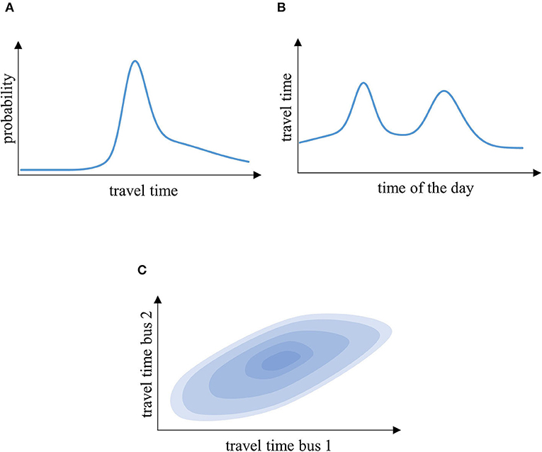
Figure 1. Typical representation explaining (A) day-to-day variability, (B) variability over the course of a day, and (C) vehicle-to-vehicle variability.

The second type of variability, variability over the course of the day (also known as inter-period or period-to-period variability), describes variability between vehicles making similar trips at different times on the same day. As shown in Figure 1B, bus travel times are usually longer for a given trip during peak periods compared with off-peak periods. The variability over the course of the day can be caused by short-term changes in congestion, incidents, or weather conditions.

Finally, the third type of variability, vehicle-to-vehicle (or inter-vehicle) variability, describes the variability between travel times experienced by different vehicles traveling at similar times over the same route. For example, Figure 1C compares the travel times of two subsequent vehicles. Vehicle-to-vehicle variability is mainly caused by different delay times at traffic signals, conflicts with pedestrians, or differences in driving behavior. It can also be used as an indicator for detecting bus bunching.

Most studies considering variability of travel times focus exclusively on the day-to-day variability. The reason for this is that commuters travel with a specific service at a specific time on multiple days. Also for operators, the day-to-day variability is of key interest, as it shows the performance on multiple days and represents the starting point for schedule optimizations and allocating slack times.

The reliability of public transport service is a very important factor in passenger satisfaction and is closely linked with travel time variability. While there is no commonly accepted definition of reliability (Carrion and Levinson, 2012), it is generally used in the transport literature to describe the stability, certainty, and predictability of travel conditions (Mattsson and Jenelius, 2015). Four specific measures for bus reliability are travel time variability, headway variability, passenger wait time variability, and punctuality (Sorratini et al., 2008). From the passengers' point of view, the regularity is an important measure of reliability. Especially in the context of high-frequency services, passengers typically arrive randomly at stops without consulting the timetable (Cats, 2014). Continuous statistical distributions are attractive because their statistical parameters are simple, and can describe elegantly the shape and extent of the travel time distribution, and reproduce it for prediction and control purposes.

Travel time variability regarding bus travel can be assessed using empirical standard deviations (Abkowitz and Engelstein, 1983; Mazloumi et al., 2010). This feature cannot comprehensively represent the stochastic features of travel times, since some features (e.g., skewness and multimodality), are missing (see the example for cars in Van Lint et al., 2008). Therefore, Kieu et al. (2014) proposed two public transport-oriented definitions of travel time variability, one for a corridor-level and the second at a service-level. They suggest the use of lognormal distributions to calculate the proposed indicators of variability.

Components of Travel Times and Their Variability

This section defines the spatial and time components of a public transport route that are used in this review. The spatial definitions of a bus route are illustrated in Figure 2. As shown, a bus travels from an origin terminal to a destination terminal passing through a set of bus stops along the way. The link between two consecutive stops is called a section. All sections from an origin to a destination form a route. A segment consists of several consecutive sections.

FIGURE 2

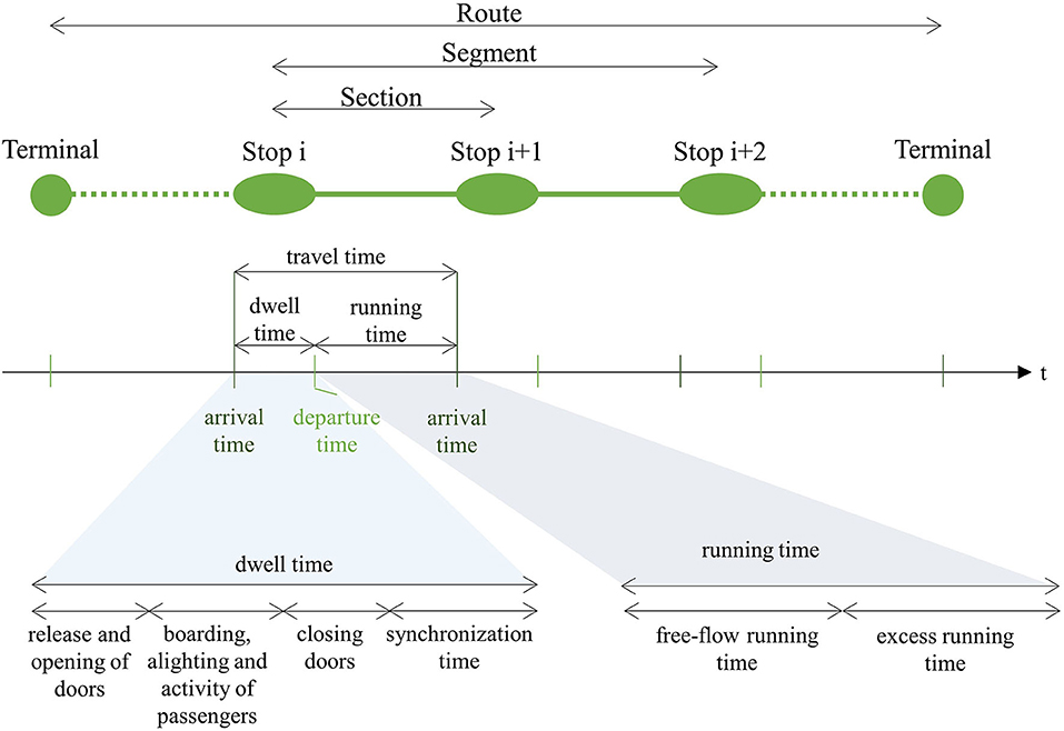
Figure 2. Spatial definitions of a bus line, and components of travel, dwell, and running times.

The aforementioned definitions of travel time are seen from an operator's perspective. From a passenger's perspective, the trip travel time also includes the access time, the waiting time, and the transferring time. Modeling all passenger trip time components is, however, beyond the scope of this review, which focuses only on the operational times. While travel time and its components are durations, points in time are also interesting from a passenger and an operational point of view, namely the arrival time and the departure time at bus stops. These times can be directly calculated by summing up travel time components if one point in time is given.

The operating times can be expressed on a section, segment, or route level. The temporal definitions used in this review are illustrated in Figure 2. We take on this review only the view from the operator and neglect the view of passengers, which would also include access, egress, transfer time, route, and departure time choice. The travel time consists of the dwell time (the time a bus spends stopped at a planned stop) and the running time (the time a bus is not stopped at a stop). The travel time in a segment corresponds to the sum of the running and dwell times of a bus in the segment under consideration.

As shown in Figure 2, the dwell time can be subdivided into four subprocess components: time spent on opening the doors, boarding, alighting, and other passenger activities such as fare payment, closing the doors, and synchronization time. Synchronization time is the time early-arriving vehicles spend waiting at control points to return to their schedule. Running time can be subdivided into two categories: the free-flow running time (i.e., the minimum time a bus needs to travel from one bus stop to the next) and the excess running time caused by traffic conditions or traffic signals along the route.

Dwell times are highly dependent on the number of passengers served. Additional factors influencing dwell time are the number of passengers on board, vehicle characteristics such as number of doors, passenger behavior, driver behavior, fare collection methods, and bus lift operations (Dueker et al., 2004).

Running times, on the other hand, depend on the infrastructure configuration (e.g., dedicated bus lanes or signal priority) and traffic conditions. Additional factors influencing running time are driver behavior, weather, and schedule quality (Abkowitz and Engelstein, 1983; Levison, 1983). All the factors influencing dwell time and running time are stochastic in nature and challenging to quantify (e.g., separating driver behavior from road traffic context).

As dwell times and running times are affected by different factors, it is meaningful to investigate them separately (see Wong and Khani, 2018). Mazloumi et al. (2010) explain this in a practical example: Early running buses wait at timing points until their predefined scheduled departure time. This leads to a longer left tail in the travel time distributions compared with the running time distribution. Hence, separating running and dwell times helps to understand the reasons for the variation of these random variables. Investigating travel time distributions has the advantage that the data does not have to be available at the running and dwell time level. Furthermore, passengers are specifically interested in segment-based travel times (the time they spend in the bus; Xue et al., 2011), whereas the split in dwell and running times is more of interest for operators.

In this study, we review papers that interpret the variability as a whole. The individual contribution of the influencing factors toward the distribution of travel times is not in the scope of this study. A variety of studies aim to identify and model these factors, as they are vital for describing and predicting travel times. Parametric statistical approaches (e.g., hazard-based approaches) are a comprehensive approach to model these factors (Anastasopoulos et al., 2017).

Literature Analysis

Methodology

This systematic literature review aims to report the state of the field of modeling statistical distributions to bus travel time and components of bus travel time observations. In this section, we report the steps of the systematic literature review.

To identify relevant publications, we performed a snowball search in the following databases: ScienceDirect, Web of Science, SCOPUS, and Google Scholar. We used multiple databases in order to identify a greater diversity of papers. A combination of keywords to state the model (keywords: “public transport” and “bus”), the considered observation (keywords: “travel time,” “running time,” and “dwell time”), and the model (keywords: “variability,” “reliability,” “distributions,” and “statistical modeling”) was used. Furthermore, common alterations of the keywords were considered, e.g., “transport” and “transportation.” This search for the chosen keywords was directed in the databases, if possible, for the title, abstract, and keywords. We considered snowballing by means of the reference list of the found papers. Since this topic is relevant for public transport systems throughout the world, consequently, a specific geographical constraint was not applied.

Any study included in this review needs to fulfill the following criteria: it needs to be a journal article or conference proceeding published in English that proposed statistical distributions based on empirical findings from case studies. The found papers were reviewed manually to strictly conform to the inclusion criteria.

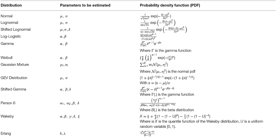
To standardize the literature information, this paper adopts the matrix method to extract key factors, by which the publications differ or accord. In the following, we first look at the studies that investigate the travel time as a whole. In the subsequent sections, we look at the studies that investigate only the travel time components, i.e., the dwell time and the running time. Various statistical distributions are proposed. For the readers' convenience, we listed the proposed statistical distributions in Appendix A.

Travel Time

In an early work, Taylor (1982) manually collected travel time data from 15 successive daily home to work trips commencing at 8:15 a.m. each day. The research has intensified in the last decade as data has become easier to collect and analyze. Recent studies incorporate larger data sets to analyze and model bus operations: for example, Mazloumi et al. (2010) consider 3,351 bus runs and Dai et al. (2019) consider 2,932 bus runs.

While most data was originally collected by hand (Taylor, 1982), today data can be collected using AVL and GPS systems, which provide precise time and position information for vehicles at stops or in-motion. Still, the massive amount of data is often reduced to the arrival and the departure time. Another method for collecting bus position information is transit signal priority data (Kieu et al., 2014), which provide bus position information at certain locations.

Similar to car traffic, bus travel times vary over the course of a day. Typically, running and dwell times and the variations in these times are higher during peak periods. Given this variation, most of the studies reviewed for this research only consider one period or treat periods of the day separately (Xue et al., 2011; Cats et al., 2014; Kieu et al., 2014; Durán-Hormazabal and Tirachini, 2016; Ma et al., 2016; Yan et al., 2016; Chen and Sun, 2017; Chepuri et al., 2018; Rahman et al., 2018; Wong and Khani, 2018). Some studies further aggregate travel time observations into departure time windows (DTW). Another approach is to only consider specific buses (Taylor, 1982; Kieu et al., 2014). Out of all the considered studies, only Dai et al. (2019) aggregated all measured data for the entire day rather than focusing on a specific time period or DTW.

The distributions of travel times are investigated on different spatial aggregation levels. Whereas, Kieu et al. (2014) investigated section travel times, others such as Chen and Sun (2017) focus on segment travel times; other studies, e.g., Mazloumi et al. (2010), consider route travel times.

The studies tested numerous different distributions for estimating travel time variability and made different recommendations for the best distribution. The normal, lognormal, or log-logistic were frequently proposed to be the best distribution for conventional distributions.

Recent automobile traffic research suggests the use of mixture distributions for fitting travel time distributions (Guo et al., 2010; Susilawati et al., 2013). This is because Van Lint and Van Zuylen (2005) identified for private vehicles four phases (free-flow conditions, congestion onset, congestion, and congestion dissolve) that yielded distinctively different shapes of travel time variability. Ma et al. (2016) adapted this approach to bus travel times. They used Gaussian mixture models with up to three components, namely free-flow, recurrent, and non-recurrent traffic state for describing the probability distributions. Similarly, Chen and Sun (2017) fitted mixture distributions to travel time of buses to account for different traffic states. Their results showed that a four-component model worked best at representing the data during peak hours and a two-component model worked best during off-peak hours. However, it remained unclear how the observed components can be allocated to service states or phases.

Table 1 summarizes the key characteristics of the reviewed research. The characteristics shown are data collection method, study area, time of the day when the study was performed, DTW (departure time window, i.e., temporal aggregation level), and spatial aggregation (section, segment, and route). Finally, the proposed distributions and the number of component distributions are specified.

TABLE 1

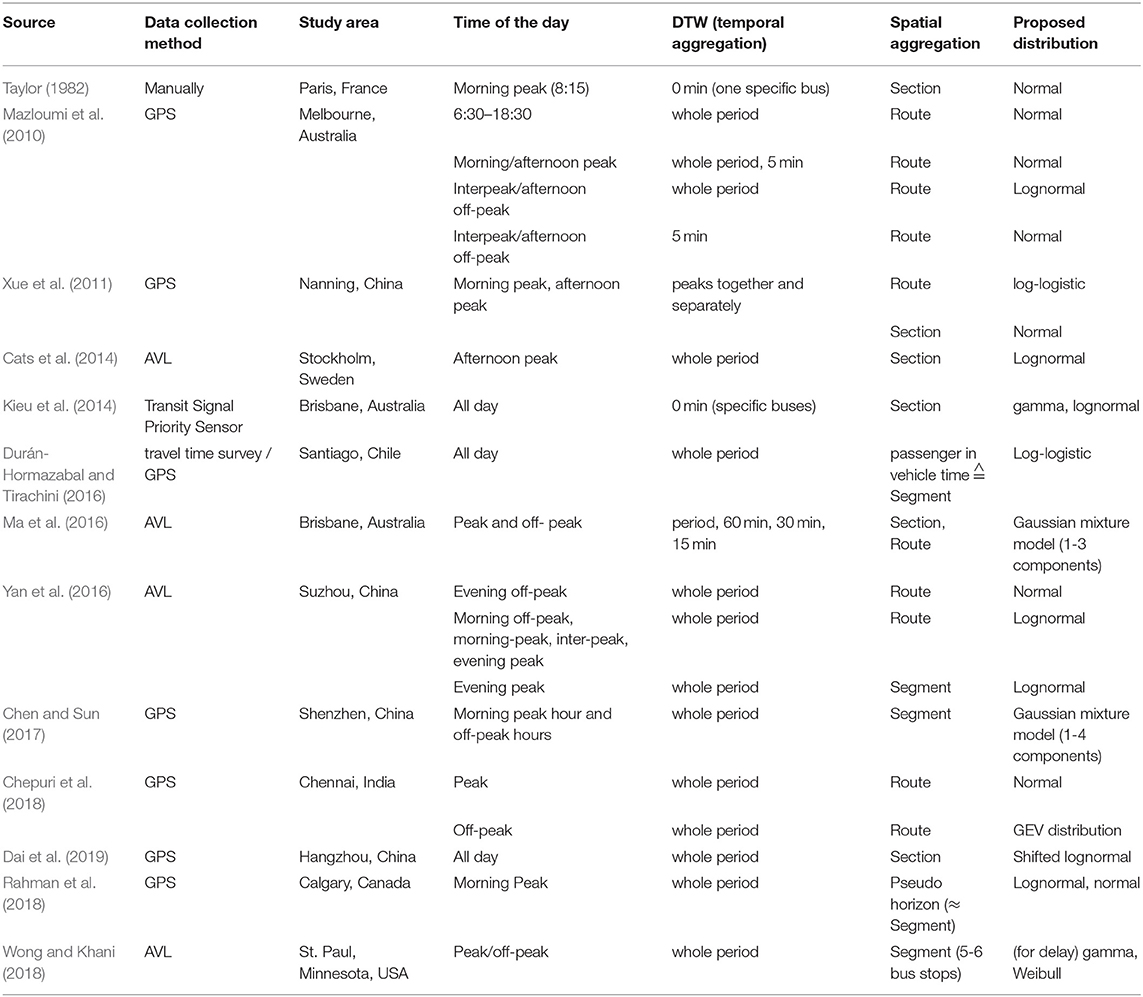
Table 1. Compilation of studies examining travel times.

Running Time

In contrast to automobile traffic, only a limited number of studies have been conducted to empirically understand which distributions are suitable for modeling bus running times. The first studies of automobile travel times proposed symmetrical continuous distributions, in particular the normal distribution, to characterize vehicle travel time on a link level. However, further research pointed out that travel time distributions are asymmetric and considerably right-skewed (Richardson and Taylor, 1978). More recent research recommends using the lognormal distribution due to its good fit and the fact that it is characterized by only two parameters (Xue et al., 2011). When buses share the same road space with automobiles and have similar characteristics (e.g., maximal speed), there is a strong similarity between automobile travel time and bus running time. Under these conditions, it is logical that the statistical modeling of both means of transport can also be similar. Therefore, most research recommends the use of lognormal distributions are proposed to statistically model running times of buses (Uno et al., 2009; Mazloumi et al., 2010; Xue et al., 2011).

However, an early study by Jordan and Turnquist (1979), which investigated the running time of buses in the morning peak in Chicago, USA, recommended using a shifted gamma distribution, where the shift equals the minimum motion time. Consequently, the gamma distribution essentially represents the delay, whereas the travel time consisted of a deterministic part (minimum motion time) and a stochastic part (excess running time). Table 2 summarizes the key characteristics of the reviewed publications considering bus running times.

TABLE 2

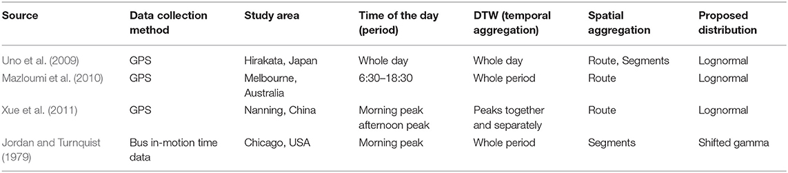
Table 2. Compilation of studies examining running times.

Dwell Time

Most of the literature models the dwell time as a function of the number of boarding and alighting passengers as well as the crowdedness (Dueker et al., 2004; Tirachini, 2013). Some works include additional factors such as the bus type. Very few studies directly address modeling statistical distributions of bus dwell times. Jiang and Yang (2014) performed video analysis of three bus stops during peak hours in Shanghai, and proposed using an Erlang distribution to fit the data. Li et al. (2012) studied the dwell times in Changzhou, and proposed using a lognormal distribution. The lognormal distribution was also proposed by Rajbhandari et al. (2003), who studied dwell times in New Jersey, USA. Koshy and Arasan (2005) proposed using a normal distribution for dwell time data from a curbside bus stop in Chennai City, India.

Khoo (2013) investigated the influence of various parameters on the dwell time distribution. They found that the Pearson 6 distributions yield the best fit to the data for both peak and off-peak conditions. They furthermore investigated the effects of platform crowding level and suggested Weibull distribution for less crowded situations and the Pearson 6 distribution for crowded situations. Rashidi and Ranjitkar (2013) investigated bus dwell time data collected by an AVL system in Auckland, New Zealand and concluded that the data is well-represented by the Wakeby distribution. In addition, they found that lognormal distribution performed satisfactorily while using a normal distribution was not suitable for estimating dwell time. Finally, Wong and Khani (2018) fitted different distributions to dwell times. However, they could not identify which yields the best fit using Cullen-Frey graphs. Table 3 summarizes the key characteristics of the reviewed publications considering bus dwell times.

TABLE 3

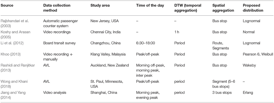
Table 3. Compilation of studies examining dwell times.

Discussion

Descriptive Analytics: Spatiotemporal Aggregation

Bus operations show remarkable variations over the course of a day, with typically larger running times and dwell times, as well as their variations, during peak conditions. Figure 3 shows a typical graph of the mean and the variation of the route travel time of buses over the course of a day. Hence, the distribution of travel time components depends on the temporal aggregation.

FIGURE 3

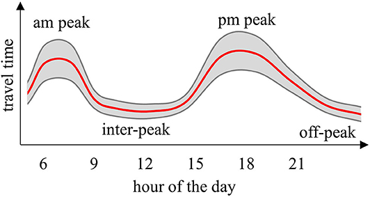
Figure 3. Typical changes of the mean (red) and the variation (gray) of route bus travel times over the course of the day.

Mazloumi et al. (2010) investigated the effects of the temporal aggregation of bus travel time data by aggregating the data into departure time windows (DTWs). This allowed them to examine the travel time distributions for DTWs at different times of the day. Their study showed that for narrow DTWs, travel time distributions are best characterized by normal distributions, while for wide DTWs, peak-hour travel times are well-represented by normal distributions, and off-peak travel times seem to follow lognormal distributions. Ma et al. (2016) also concluded that increasing the temporal aggregation of travel times tends to make distributions more asymmetric and to decrease the normality of distributions. In fact, as the temporal aggregation attribute is increased, some of the variability within the course of a day is incorporated into the day-to-day variability.

The spatial aggregation also significantly influences the distribution of travel time components. For example, Ma et al. (2016) investigated section level and route level distributions. They found that section level travel times are often multi-modal, whereas route travel times seem to be rather unimodal. In other words, the multi-modality of the distribution on a section level seems to be eliminated when the data is aggregated on a route level. This can be explained by the ability of the driver to speed up in successive sections to catch up with the timetable, especially if buses have the exclusive right of way, where drivers can precisely control speed.

Rahman et al. (2018) used a slightly different approach to show the influence of spatial aggregation. They worked with GPS-data and defined the term pseudo horizon as the distance from a GPS point to an upstream GPS point on the same route. Then, they analyzed the changes in bus travel time characteristics as the pseudo horizon varies. They found that at a range of 8 km (a boundary probably depending on the topology of the network and operations), there is a significant change in bus travel time characteristics. The travel time distributions of buses converge from a rightly skewed distribution to a more symmetrical distribution from shorter to longer pseudo horizons. They recommend lognormal distributions for pseudo-horizons of under 8 km and normal distributions for longer pseudo-horizons. Xue et al. (2011) contradict this finding by stating that the kurtosis and skewness of the distribution become larger for longer segments, but do not provide an explanation for this behavior. However, generally, with the exception of Xue et al. (2011), studies agree that smaller spatial aggregation leads to higher skewness values and more variability.

The combination of section travel times into route travel time needs to incorporate correlation effects into successive sections. Spatial regression models have been used for this purpose for automobile traffic, e.g., Hackney et al. (2007). Additionally, it is also interesting to study how the knowledge of a distribution is affected given some additional information over time (the approach in Corman and Kecman, 2018).

Figure 4 illustrates the spatial and temporal aggregation levels of the studies reviewed in this research, which target different spatial and time aggregations, and are therefore hard to compare directly. Studies that systematically investigate either the influence of the temporal or the spatial aggregation are shown with dotted borders. Since none of the studies investigated spatial and temporal aggregation at the same time, it is unknown which type of aggregation has greater effects on the travel time variability and choice of distribution model. Figure 4 furthermore points to a research gap in studying subsequent buses, i.e., descriptive analytics for studying bus bunching.

FIGURE 4

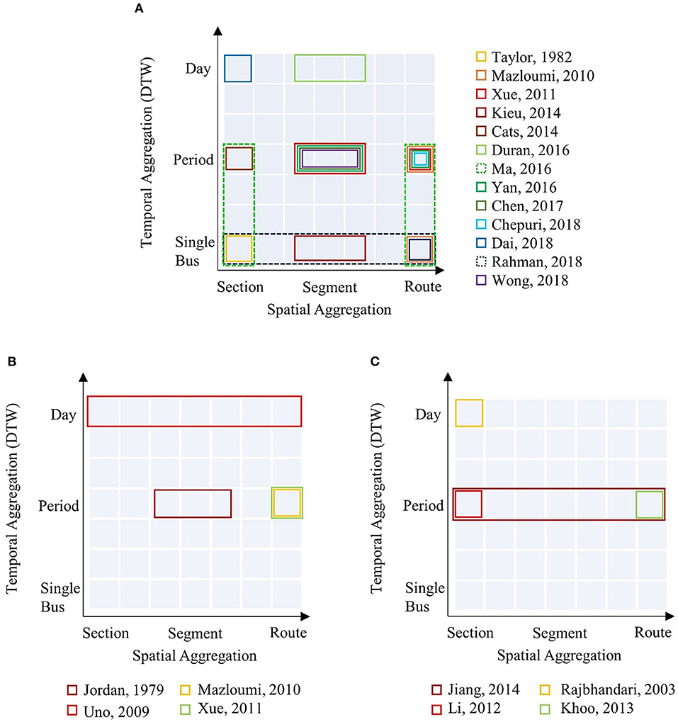
Figure 4. Representations of spatial and temporal aggregation of (A) travel time, (B) running time, and (C) dwell time.

When considering route travel times at peak period, Mazloumi et al. (2010) and Chepuri et al. (2018) propose normal distributions, while Ma et al. (2016) and Chen and Sun (2017) propose Gaussian mixture models, and Yan et al. (2016) propose lognormal distributions (see Figure 4A). For short segments, skewed distributions such as log-logistic (Durán-Hormazabal and Tirachini, 2016) or lognormal (Kieu et al., 2014; Rahman et al., 2018) perform better than normal distributions.

Figure 4B presents studies of running times. Only Uno et al. (2009) conducted analysis on different levels of spatial aggregation, demonstrating that the lognormal distribution always provides the best fit. Figure 4C presents studies of dwell times. In this case, however, no systematic study on the influence of temporal or spatial aggregation has been conducted.

The main reasons for investigating the different aggregation level come from the differing interests of passengers and operators. Passengers are interested in the time they will spend on a bus, hence, they are interested in segment travel times (Xue et al., 2011). Operators, on the other side, are interested in all spatial aggregation levels. Also, concerning the temporal aggregation of travel times, the interest of operators and passengers differs. Passengers are mostly interested in short departure time windows to understand the travel times at a specific hour of the day (e.g., Yan et al., 2016) or even of a specific bus (e.g., Taylor, 1982). Operators might be interested, depending on their analyses, in period-level or single bus aggregation (e.g., Ma et al., 2016). Temporal aggregation on the level of whole days can be used as a benchmark for networkwide analyses (e.g., Durán-Hormazabal and Tirachini, 2016) and for reporting to funding agencies.

Descriptive Analytics: Type and Modality of Distributions

Unfortunately, it is not common for the authors to give clear reasons why they test and choose a certain statistical distribution. However, they often clearly state that the distributions can never perfectly model observed distributions, but only approximate them.

A first consideration in identifying an appropriate distribution is to decide whether the process being modeled has bounds. Intuitively, the running time, hence the travel time, has a minimal bound given by the maximum possible speed of a bus traveling from one stop to the next. Jordan and Turnquist (1979) applied this process by shifting their proposed (gamma) distribution by the free-flow travel time buses take to traverse the section. Dai et al. (2019) also applied shifted (lognormal) distributions. Similarly, there is the minimum bound for the dwell time, given as the process time, i.e., the time spent on opening and closing the doors. However, none of the publications investigating distributions of dwell times incorporated a lower bound greater than zero. This should suggest using right-skewed distributions rather than symmetrical (e.g., Gaussian) ones.

One of the most discussed considerations in finding a distribution is determining whether the distribution should be modeled as a single component distribution or a mixture distribution made up by multiple components. Recent publications suggest using mixture models, which are capable of linking the shape of the travel time distribution to the underlying travel time states. For example, Ma et al. (2016) modeled travel times with Gaussian mixture models, where the maximum number of components is set to be three. Unfortunately, it is not clear in this study how many components were actually used. In any case, such a model will always have an equal or even a better fit than a normal distribution. Chen and Sun (2017) further elaborated on the number of components used, related to the observed service states. However, their results showed that using threeå to four components for peak conditions and one to two components for off-peak conditions yield the best fit to the data. Finally, choosing mixture distributions does not answer the question on which particular distributions should be used.

Predictive Analytics: Distribution Fitting and Choice of Reproducible Distribution

A variety of different methodologies for identifying the most suitable statistical distribution to model the travel time and its components were used in the studies reviewed for this research. First, the parameters of candidate distributions have to be estimated. This is mostly done by the maximum likelihood estimation (MLE). Other parametric methods as method of moments or regression methods were not applied. After estimating these parameters, typical hypothesis tests such as Anderson-Darling (Ma et al., 2016), Kolmogorov-Smirnov (Mazloumi et al., 2010), or chi-squared (Khoo, 2013) are used. These tests have different limitations.

A major limitation of Kolmogorov-Smirnov and Anderson-Darling tests is that they are not valid if parameters are directly estimated from the tested data. This limitation can be resolved by using a bootstrap procedure as (presented in Stute et al., 1993, and used in Kieu et al., 2014). Another approach is to divide the measured data into a training set, used to estimate the parameters, and a testing set, which is used to test the fit.

A second major limitation is the interpretation of p-values. Here, the frequently used threshold of α = 5% is not well-founded since a conclusion is not automatically “true” on one side of the threshold nor “false” on the other side (Wasserstein and Lazar, 2016). Furthermore, since the p-value depends on the sample size, it is often possible to find a tiny difference between two results that is statistically significant, but where there is no meaning in this difference within the empirical context. This is especially problematic for bus travel time studies where huge amounts of AVL or GPS data are available. Therefore, it is important to communicate the effect size (Fritz et al., 2012). In other words, it is not most important if a candidate distribution is the “true” distribution, but rather how good the distribution is in giving information about the travel time components.

To evaluate which distribution yields the best fit to a given data, different fitted distributions can be cross-compared. This can be done by choosing the distribution that shows the highest likelihood. The problem with this approach is that distributions with more parameters generally yield a better fit in comparison to distributions with fewer parameters. To overcome this problem, various studies use the Bayesian Information Criterion (BIC) or the Akaike Information Criterion (AIC). Both criteria measure the relative quality of a fit and including the number of parameters used.

Prescriptive Analytics: Controlled Bus Operation

An important application of travel time distributions is in developing predictive applications for improving performance. This pertains to buses running to a fixed schedule, buses running on frequency, and to a certain extent also dial-a-ride services; as far as the vehicles will be relatively large, having multiple stops along their trajectory, and subject to pending traffic conditions, we expect the same dynamics will apply (e.g., Alonso-Mora et al., 2017). For example, variations in bus travel time can lead to variation in bus headway (e.g., Newell and Potts, 1964). This instability in headways can cause bus bunching since a lagging bus must collect more passengers, and therefore tends to fall further behind. Bus bunching can be analyzed by considering headway variability (Moreira-Matias et al., 2012), bus-to-bus travel or dwell time variability (see Figure 1C). Furthermore, correlations would provide meaningful insight in helping to identify potential bunching patterns. To detect and reduce bus bunching, information about subsequent buses are needed. Day-to-day travel time variability gives no direct information about bus bunching, as the reported variability might come from very high-frequency dynamics (with a period of two buses, i.e., bunching phenomena, which impacts regularity) or lower frequency dynamics (e.g., periods with high travel times followed by periods with low travel times, such as peaks).

Recommendations for Further Research

Understanding Aggregation Issues

The spatial and temporal aggregation of travel time, running time, and dwell time data have an important influence on the statistics and the choice of most suitable probability distribution. However, only a few studies have systematically investigated the influence of spatial or temporal aggregation, nor the underlying correlations structures. Conducting such a study in multiple cities with the same methodology would add significant value to the current state-of-the-art and quantify the soft or hard boundaries between states or characteristics as dependent on city structure, supply, and operations. Moreover, peak and off-peak are commonly accepted boundaries, which in reality represent a continuous transition of states. Similarly, the time and space features by which the spatial correlation of travel times reduces and Gaussian assumption start to hold are mostly a continuous phenomenon. Most of those are probably related to spatial characteristics of city structures and operations. A rigorous determination of such space and time transitions would allow for a more meaningful description of traffic dynamics.

Putting Focus on the Tail of the Distribution

The evaluated studies model the distributions at normal conditions. There is no special focus put on the tail of the distributions, representing extraordinary behavior. But as even extraordinary behavior might reoccur, that could be modeled. It is imaginable that distributions and dependencies for extraordinary events could, and possibly should, be modeled differently as for normal operations.

Meaningful Choice of Distributions

Mixture distributions appear to better fit bus travel time data compared to conventional unimodal distributions, especially during peak hours. However, it is important to ensure that the components (i.e., service states) can be fully explained, which is currently not the case. From that perspective, distributions with simply more parameters would always achieve a better fit, but not necessarily result in physically meaningful parameters. Additionally, since the literature suggests that peak travel time components are skewed, skewed distributions such as a lognormal distribution should be considered in the modeling of mixture distributions.

Reproducible and Robust Distributions

In transport analysis, there is a growing interest in using available data for predictive purposes like supply planning, demand modeling, and timetable planning. Therefore, the proposed distributions should be reproducible with additional data. A good approach to determine the best statistical distribution should be based on a training-testing approach to avoid overfitting the data.

Incorporating Control Strategies

Bus operators use various control strategies to maintain service reliability (see Ibarra-Rojas et al., 2015). Most operators set control points along a bus route where bus departure times are subject to regulation, or have specific buffer time. Buses that arrive ahead of schedule wait at these control points to return to the schedule. This reduces the variation of the departure time at the control points. This strategy has a major effect on the day-to-day variation of travel time components, as the travel process at those points includes also a possible waiting time for the scheduled departure time. Further analysis should investigate the variation of bus travel times depending on the control strategy, buffers, and holding points.

Conclusions

This article reports on the modeling of bus running, dwell, and travel time. The importance of this topic is crucial not only for the short term improvement of existing public transport services, but even more for a future of increased automation and connectivity in vehicles. We assume in fact that future road-based transport systems, regardless of them having a driver or not, will have similar operating conditions to current buses. This means that they make use of large vehicles capable of bundling the demand efficiently. They will be partially subject to prevailing traffic dynamics and congestion related to peak hours and they will be stop-based, including multiple stops along a generalized circulation to allow people boarding and alighting. They will have a range of operations from pure schedule-based, to frequency-based, to partially demand-responsive, and they might have a varying degree of reserved infrastructure. To this end, we review the current practice for statistically modeling distributions of bus travel time components, pointing to new approaches and models needed for descriptive, predictive, and prescriptive analytics purposes in the context of bus operations.

Spatial and temporal aggregation of data have an important influence on the statistics as well as on the choice of the most appropriate probability distribution. A graphical summary of the findings from the previous section is reported in Figure 5, addressing descriptive analytics (left; how to model what) and predictive and prescriptive analytics (right: how to ensure predictive power of future operations; and how to support decision making). This calls for flexible models, which can be used and adapted for different locations and times, are able to give the information on non-stationary probability distributions, and remain with good performance through expected and unexpected technological changes.

FIGURE 5

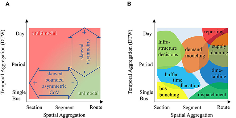
Figure 5. Graphical summary of results from the literature and recommended research Partlabels: (A) Descriptive Analytics, (B) Prescriptive/Predictive Analytics.

The parameters of the model should be relevant and should explain the conditions of the transport network; in addition, overfitting should be prevented. In general, simple models are better, as the required parameters are then easier to understand. Using mixture distributions for modeling distributions of the travel time and its components is a promising path. However, it is important that the components remain meaningful. The determination regarding the best-fitting distribution could be made using training and testing approaches. These approaches need to be further developed but are especially promising because the most important quality for a distribution is its reproducibility. It is important to seize the opportunity that the era of big data provides us in terms of transport analysis, since data is the best resource we get to approximate the truth.

Author Contributions

BB and FC contributed to the analysis of the current state of the research, discussion of results, and the writing of the manuscript.

Conflict of Interest

The authors declare that the research was conducted in the absence of any commercial or financial relationships that could be construed as a potential conflict of interest.

References

Abkowitz, M. D., and Engelstein, I. (1983). Factors affecting running time on transit routes. Transport. Res. Part A, 17, 107–113. doi: 10.1016/0191-2607(83)90064-X

CrossRef Full Text | Google Scholar

Alonso-Mora, J., Samaranayake, S., Wallar, A., Frazzoli, E., and Rus, D. (2017). On-demand high-capacity ride-sharing via dynamic trip-vehicle assignment. Proc. Natl. Acad. Sci. U.S.A. 114, 462–467. doi: 10.1073/pnas.1611675114

PubMed Abstract | CrossRef Full Text | Google Scholar

Anastasopoulos, P. C., Fountas, G., Sarwar, M. T., Karlaftis, M. G., and Sadek, A. W. (2017). Transport habits of travelers using new energy type modes: a random parameters hazard-based approach of travel distance. Transportation Res. Part C 77, 516–528. doi: 10.1016/j.trc.2017.01.017

CrossRef Full Text | Google Scholar

Bates, J., Polak, J., Jones, P., and Cook, A. (2001). The valuation of reliability for personal travel. Transport. Res. Part E, 37, 191–229. doi: 10.1016/S1366-5545(00)00011-9

CrossRef Full Text | Google Scholar

Carrion, C., and Levinson, D. (2012). Value of travel time reliability: a review of current evidence. Transport. Res. Part A 46, 720–741. doi: 10.1016/j.tra.2012.01.003

CrossRef Full Text | Google Scholar

Cats, O. (2014). Regularity-driven bus operation: principles, implementation and business models. Transport Policy 36, 223–230. doi: 10.1016/j.tranpol.2014.09.002

CrossRef Full Text | Google Scholar

Cats, O., Ru, F. M., and Koutsopoulos, H. N. (2014). Optimizing the number and location of time point stops. Public Transport 6, 215–235. doi: 10.1007/s12469-014-0092-1

CrossRef Full Text | Google Scholar

Chen, S., and Sun, D. (2017). A multistate-based travel time schedule model for fixed transit route. Transport. Lett. 1–10. doi: 10.1080/19427867.2016.1271546

CrossRef Full Text | Google Scholar

Chepuri, A., Ramakrishnan, J., Arkatkar, S., Joshi, G., and Pulugurtha, S. S. (2018). Examining travel time reliability-based performance indicators for bus routes using GPS-based bus trajectory data in India. J. Transport. Eng. 144:04018012. doi: 10.1061/JTEPBS.0000109

CrossRef Full Text | Google Scholar

Corman, F., and Kecman, P. (2018). Stochastic prediction of train delays in real-time using Bayesian networks. Transport. Res. 95, 599–615 doi: 10.1016/j.trc.2018.08.003

CrossRef Full Text | Google Scholar

Dai, Z., Ma, X., and Chen, X. (2019). Bus travel time modelling using GPS probe and smart card data: a probabilistic approach considering link travel time and station dwell time. J. Intell. Transport. Syst. 23, 175–190. doi: 10.1080/15472450.2018.1470932

CrossRef Full Text | Google Scholar

Dueker, K., Kimpel, T., Strathman, J., and Callas, S. (2004). Determinants of bus dwell time. J. Public Transport. 7, 21–40. doi: 10.5038/2375-0901.7.1.2

CrossRef Full Text | Google Scholar

Durán-Hormazabal, E., and Tirachini, A. (2016). Estimation of travel time variability for cars, buses, metro and door-to-door public transport trips in Santiago, Chile. Res. Transport. Econ. 59, 26–39. doi: 10.1016/j.retrec.2016.06.002

CrossRef Full Text | Google Scholar

Fritz, C. O., Morris, P. E., and Richler, J. J. (2012). Effect size estimates: current use, calculations, and interpretation. J. Exp. Psychol. 141, 2–18. doi: 10.1037/a0024338

PubMed Abstract | CrossRef Full Text | Google Scholar

Guo, F., Rakha, H., and Park, S. (2010). Multistate model for travel time reliability. Transport. Res. Record 2188, 46–54. doi: 10.3141/2188-06

CrossRef Full Text | Google Scholar

Hackney, J. K., Bernard, M., Bindra, S., and Axhausen, K. W. (2007). Predicting road system speeds using spatial structure variables and network characteristics. J. Geogr. Syst. 9, 397–417. doi: 10.1007/s10109-007-0050-4

CrossRef Full Text | Google Scholar

Ibarra-Rojas, O. J., Delgado, F., Giesen, R., and Muñoz, J. C. (2015). Planning, operation, and control of bus transport systems: a literature review. Transport. Res. Part B 77, 38–75. doi: 10.1016/j.trb.2015.03.002

CrossRef Full Text | Google Scholar

Jiang, X., and Yang, X. (2014). “Regression-based models for bus dwell time,” in Intelligent Transportation Systems (ITSC), 2014 IEEE 17th International Conference on. IEEE. 2858–2863.

Google Scholar

Jordan, W. C., and Turnquist, M. (1979). Zone scheduling of bus routes to improve service reliability. Transport. Sci. 13, 242–268. doi: 10.1287/trsc.13.3.242

CrossRef Full Text | Google Scholar

Khoo, H. L. (2013). Statistical modeling of bus dwell time at stops. J. Eastern Asia Soc. Transport. Stud. 10. 1489–1500. doi: 10.11175/easts.10.1489

CrossRef Full Text | Google Scholar

Kieu, L.-M., Bhaskar, A., and Chung, E. (2014). Public transport travel-time variability definitions and monitoring. J. Transport. Eng. 141:04014068. doi: 10.1061/(ASCE)TE.1943-5436.0000724

CrossRef Full Text | Google Scholar

Koshy, R. Z., and Arasan, V. T. (2005). Influence of bus stops on flow characteristics of mixed traffic. J. Transport. Eng. 131, 640–643. doi: 10.1061/(ASCE)0733-947X(2005)131:8(640)

CrossRef Full Text | Google Scholar

Levison, H. (1983). Analyzing transit travel time performance. Transportation Research Record 915.

Google Scholar

Li, F., Duan, Z., and Yang, D. (2012). Dwell time estimation models for bus rapid transit stations. J. Modern Transport. 20, 168–177. doi: 10.1007/BF03325795

CrossRef Full Text | Google Scholar

Li, Z., Hensher, D. A., and Rose, J. M. (2010). Willingness to pay for travel time reliability in passenger transport: a review and some new empirical evidence. Transport. Res. Part E 46, 384–403. doi: 10.1016/j.tre.2009.12.005

CrossRef Full Text | Google Scholar

Ma, Z., Ferreira, L., Mesbah, M., and Zhu, S. (2016). Modeling distributions of travel time variability for bus operations: bus travel time distribution model. J. Adv. Transport. 50, 6–24. doi: 10.1002/atr.1314

CrossRef Full Text | Google Scholar

Mattsson, L. G., and Jenelius, E. (2015). Vulnerability and resilience of transport systems–a discussion of recent research. Transport. Res. Part A 81, 16–34. doi: 10.1016/j.tra.2015.06.002

CrossRef Full Text | Google Scholar

Mazloumi, E., Currie, G., and Rose, G. (2010). Using GPS data to gain insight into public transport travel time variability. J. Transport. Eng. 136, 623–631. doi: 10.1061/(ASCE)TE.1943-5436.0000126

CrossRef Full Text | Google Scholar

Moreira-Matias, L., Ferreira, C., Gama, J., Mendes-Moreira, J., and de Sousa, J. F. (2012). Bus bunching detection by mining sequences of headway deviations. Adv. Data Mining 7377, 77–91. doi: 10.1007/978-3-642-31488-9_7

CrossRef Full Text | Google Scholar

Newell, G. F., and Potts, R. B. (1964). “Maintaining a bus schedule,” in Australian Road Research Board (ARRB) Conference, 2nd, 1964, Melbourne (Vol. 2, No. 1).

Google Scholar

Noland, R. B., and Polak, J. W. (2002). Travel time variability: a review of theoretical and empirical issues. Transport Rev. 22, 39–54. doi: 10.1080/01441640010022456

CrossRef Full Text | Google Scholar

Rahman, M. M., Wirasinghe, S., and Kattan, L. (2018). Analysis of bus travel time distributions for varying horizons and real-time applications. Transport. Res. Part C 86, 453–466. doi: 10.1016/j.trc.2017.11.023

CrossRef Full Text | Google Scholar

Rajbhandari, R., Chien, S., and Daniel, J. (2003). Estimation of bus dwell times with automatic passenger counter information. Transport. Res. Record 120–127. doi: 10.3141/1841-13

CrossRef Full Text | Google Scholar

Rashidi, S., and Ranjitkar, P. (2013). Approximation and short-term prediction of bus dwell time using AVL data. J. Eastern Asia Soc. Transportation Stud. 10, 1281–1291. doi: 10.11175/easts.10.1281

CrossRef Full Text | Google Scholar

Richardson, A., and Taylor, M. (1978). Travel time variability on commuter journeys. High Speed Ground Transport. J. 12, 77–99. Available online at: https://trid.trb.org/view/80100

Google Scholar

Sorratini, J., Liu, R., and Sinha, S. (2008). Assessing bus transport reliability using micro-simulation. Transport. Plann. Technol. 31, 303–324. doi: 10.1080/03081060802086512

CrossRef Full Text | Google Scholar

Stute, W., Manteiga, W. G., and Quindimil, M. P. (1993). Bootstrap based goodness-of-fit-tests. Metrika 40, 243–256. doi: 10.1007/BF02613687

CrossRef Full Text | Google Scholar

Susilawati, S., Taylor, M., and Somenahalli, S. V. (2013). Distributions of travel time variability on urban roads. J. Adv. Transport. 47, 720–736. doi: 10.1002/atr.192

CrossRef Full Text | Google Scholar

Taylor, M. (1982). Travel time variability—the case of two public modes. Transport. Sci. 16, 507–521. doi: 10.1287/trsc.16.4.507

CrossRef Full Text | Google Scholar

Tirachini, A. (2013). Bus dwell time: the effect of different fare collection systems, bus floor level and age of passengers. Transportmetrica A 9, 28–49. doi: 10.1080/18128602.2010.520277

CrossRef Full Text | Google Scholar

Uno, N., Kurauchi, F., Tamura, H., and Iida, Y. (2009). Using bus probe data for analysis of travel time variability. J. Intell. Transport. Syst. 13, 2–15. doi: 10.1080/15472450802644439

CrossRef Full Text | Google Scholar

Van Lint, J., and Van Zuylen, H. (2005). Monitoring and predicting freeway travel time reliability: using width and skew of day-to-day travel time distribution. Transport. Res. Record 1917, 54–62. doi: 10.1177/0361198105191700107

CrossRef Full Text | Google Scholar

Van Lint, J. W. C., Van Zuylen, H. J., and Tu, H. (2008). Travel time unreliability on freeways: why measures based on variance tell only half the story. Transport. Res. Part A 42, 258–277. doi: 10.1016/j.tra.2007.08.008

CrossRef Full Text | Google Scholar

Wasserstein, R. L., and Lazar, N. A. (2016). The ASA's statement on p -values: context, process, and purpose. Am. Statist. 70, 129–133. doi: 10.1080/00031305.2016.1154108

CrossRef Full Text | Google Scholar

Wong, E., and Khani, A. (2018). Transit delay estimation using stop-level automated passenger count data. J. Transport. Eng. 144:04018005. doi: 10.1061/JTEPBS.0000118

CrossRef Full Text | Google Scholar

Xue, Y., Jin, J., Lai, J., Ran, B., and Yang, D. (2011). “Empirical characteristics of transit travel time distribution for commuting routes,” in Transportation Research Board 90th Annual Meeting (Washington, DC). Available online at: https://trid.trb.org/view/1092692

Google Scholar

Yan, Y., Liu, Z., and Bie, Y. (2016). Performance evaluation of bus routes using automatic vehicle location data. J. Transport. Eng. 142:04016029. doi: 10.1061/(ASCE)TE.1943-5436.0000857

CrossRef Full Text | Google Scholar

Appendix A