 George C. Tsiatas
 Antonis G. Siokas
 Evangelos J. Sapountzakis
- 1Department of Mathematics, University of Patras, Rio, Greece
- 2School of Civil Engineering, National Technical University of Athens, Athens, Greece
- 3School of Civil Engineering, National Technical University of Athens, Athens, Greece
This work aims to introduce a new layered approach to the nonlinear analysis of initially straight Euler-Bernoulli beams by the Boundary Element Method (BEM). The beam is studied in the context of both geometrical and material nonlinearity. The governing differential equations, derived by applying the principle of minimum total potential energy, are coupled and nonlinear, while the boundary conditions are the most general and may include elastic support or restraint. The boundary value problem, regarding the axial and transverse displacements, is solved using the Analog Equation Method (AEM), a BEM based method, together with an iterative procedure. Although a direct solution to the geometrical nonlinear problem has already been presented, in this work an alternative layered analysis is proposed. The discretization is applied in both the longitudinal direction and the cross-sectional plane, and an iterative process is commenced. First, initial fictitious load distributions are assumed at beam's each cross-section, and the displacements, as well as their derivatives, are computed using the AEM. Second, the two stress resultants, i.e., the axial force and bending moment, are evaluated by appropriate integration over the cross-section. In the end, the derivatives of the stress resultants are evaluated, and the equilibrium of the governing equations is checked. If the equilibrium is satisfied, the process is terminated. Otherwise, the fictitious load distributions are updated, and the procedure starts over again. Several representative examples are studied, and the results are compared with those presented in the literature, validating the reliability and effectiveness of the proposed method.
Introduction
Beam elements have historically found applications in the process of structural modeling and analysis in a wide range of engineering disciplines, from civil (e.g., buildings, bridges) to mechanical (e.g., shafts, wind turbine parts, nuclear reactor components) to aeronautical (e.g., aircraft wings, spacecraft parts) (Hodges, 2006) to name only a few. For this reason, considerable research has been directed at studying the static and dynamic structural behavior of beams. Over the years, the exponential growth in computational power in conjunction with significant advances in numerical methods have led to more sophisticated simulations; the initially simplifying modeling assumptions have been gradually diminished, and more realistic nonlinear formulations are employed.
In general, two conventional sources of nonlinearity may affect the response of structural elements: material and geometrical (Reddy, 2005a). On the one hand, material nonlinearity stems from the inherent nonlinear constitutive behavior of several materials. In this case, the stress-strain relation may be a function of the combined or individual stress, strain or strain rate and may also be path dependent about the load history. Nonlinear material behavior in solid mechanics can be rate-independent or rate-dependent (Taylor, 1996). On the other hand, the geometrical nonlinearity results from maintaining the square of the slope in the strain-displacement relations (Katsikadelis and Tsiatas, 2003). In this case, the transverse deflection affects the axial force, and the resulting governing equations are coupled nonlinear with variable coefficients.
An analytical solution to the mathematical model describing the behavior of the beam cannot be obtained when general boundary conditions are imposed at its ends; therefore, a numerical approach should be adopted (Katsikadelis and Tsiatas, 2003). The most widely used numerical methods in Computational Mechanics are the Finite Element Method (FEM), the Boundary Element Method (BEM), and the Finite Difference Method (FDM) (Banerjee and Butterfield, 1981; Becker, 1992). Firstly, FDM can be applied to any system of differential equations by substituting the differential operators with algebraic ones at representative nodes after the problem domain discretization. It is the simplest of the three methods and relatively easy to program. However, it is not suitable for problems with irregular domain geometries and rapidly changing variables, due to the difficulty of establishing a non-uniform grid of nodes. Secondly, according to FEM, the domain of the solution is decomposed into a finite number of smaller subdomains, called finite elements. On each subdomain the behavior of the whole body is approximated, and then continuity and balance rules are applied at the boundaries of the elements to obtain the solution for the entire domain (Plevris and Tsiatas, 2018). FEM is appropriate for problems with geometrical complex solution domains. However, discretizing the whole body results in a large number of finite elements leading to significant computational cost. Lastly, BEM, applying the concept of the Fundamental Theorem of Calculus, transforms the governing differential equations into equivalent integral ones, thus transferring the solution domain to its boundary, where a discretization scheme is then established. In this respect, the dimension of the problem is reduced by one order while the number of unknowns is also significantly reduced (Plevris and Tsiatas, 2018). Moreover, the BEM allows the evaluation of the derivatives of the solution at any point of the original solution domain (before the initial integration), whereas it is suitable for the analysis of structures with complex boundaries and geometric peculiarities, such as cracks (Katsikadelis, 2016).
To the problem at hand, FEM has been adopted by many researchers for the materially and/or geometrical nonlinear analysis of beams. In particular, Mondkar and Powell (1977), examined structures accounting for large displacements with finite strains and formulated the incremental equations of motion using the principle of virtual displacements. Argyris et al. (1978a,b, 1979), to circumvent the complications emerging from the noncommutative nature of rotations about fixed distinct axes, presented the concept of semi-tangential rotation in the matrix displacement analysis of geometrically nonlinear structures. Bathe and Bolourchi (1979) studied the behavior of a beam element undergoing large displacements and large rotations formulating a total Lagrangian and an updated Lagrangian approach. Yang and McGuire (1986) presented a nonlinear analysis of beams with a doubly symmetric cross-section employing an updated Lagrangian finite element formulation. Cai et al. (2009) performed a large deformations-large rotations finite element analysis of a three-dimensional frame with members of arbitrary cross-sections by the nonlinear Von Karman theory of deformation.
Furthermore, linear and nonlinear analysis of beams has also been performed employing BEM. Banerjee and Butterfield (1981) and Providakis and Beskos (1986) employed BEM in order to solve the static and dynamic problems of Euler-Bernoulli beams, respectively. Further, the Analog Equation Method (AEM), a numerical technique based on BEM, was applied to the nonlinear static (Katsikadelis and Tsiatas, 2003) and dynamic (Katsikadelis and Tsiatas, 2004) flexural analysis of beams with variable cross-section. Sapountzakis and Mokos (2008) and Sapountzakis and Panagos (2008) studied the nonlinear flexural behavior of beams of doubly symmetric constant and variable cross-section using BEM and adopting the assumptions of the Timoshenko beam theory. Tsiatas (2010) examined the nonlinear problem of non-uniform beams resting on a nonlinear elastic foundation presenting a boundary integral equation solution. Sapountzakis and Dourakopoulos (2010) formulated a BEM solution to the moderate large deflections flexural-torsional analysis of Timoshenko beams of a constant cross-section of arbitrary shape under general boundary conditions. Sapountzakis and Dikaros (2011) adopted a BEM methodology to examine the effects of warping and rotary inertia to the moderate large deflections and twisting rotations flexural-torsional dynamic analysis of beams.
In formulating a one-dimensional element for the linear or nonlinear analysis of beams, two considerations have to be made: First, the prediction of the cross-sectional response. Second, the integration of the cross-sectional response over the length of the element to obtain its response regarding the available degrees of freedom (Izzuddin et al., 2002). Although the latter consideration has been extensively presented in the previous works, an open issue remains regarding the former consideration.
As far as cross-sectional response is concerned, three main approaches have been widely adopted (Izzuddin et al., 2002): According to the first one, explicit expressions for cross-sectional response parameters (e.g., stress-strain functions) are provided. The second one utilizes interaction relationships based mainly on principles of plasticity. The third approach, known as the fiber approach, utilizes a cross-sectional decomposition into a finite number of subdomains adequately small to readily evaluate stresses and strains at representative points. The fiber approach is the most general, as it can be applied even in cases where the stress-strain relation is not a priori known, or even if a mathematical function can not explicitly describe it, but only by sets of experimental data.
In this respect, the fiber model has been extensively applied in the analysis and design of beams. Kaba and Mahin (1984) first introduced a beam element divided into fibers for the analysis of reinforced concrete or steel members assuming that plane sections remain plane. They used both force and displacement shape functions to compute the element flexibility and the element-resisting forces, respectively. Filippou et al. (1991) presented a FEM solution for the problem of reinforced concrete members under cyclic loading conditions that induce biaxial bending and axial force. Zbiciak (2010) presented a formulation of an initial-boundary-value problem for the Euler-Bernoulli beam made of pseudoelastic shape memory alloy (SMA). A 2D finite difference discretization scheme was established in the longitudinal sense and on the cross-sectional plane dividing the cross-section into layers of constant thickness. More recently, Sapountzakis and Kampitsis (2017) developed a hybrid domain BEM formulation for the geometrical nonlinear analysis of inelastic Euler-Bernoulli beams resting on viscous inelastic Winkler foundation, employing an inelastic redistribution modeled through a fiber approach. Finally, Tsiatas et al. (2018) presented a first step toward the solution of the problem presented in this work, employing a fiber approach to the large deflections analysis of beams by BEM. In this solution, the material nonlinearity of the beam was not considered.
In this work, a layered approach to the nonlinear analysis of initially straight Euler-Bernoulli beams by BEM is presented. The beam is studied in the context of both geometrical and material nonlinearity. It must be noted that in the current analysis, the cross-sections under consideration are rectangular. In this case, the fiber model can be reduced to a layered model; more specifically, fibers can be substituted by layers of constant thickness. The formulation of the problem is based on the displacements, and the equations of equilibrium, derived from the principle of minimum total potential energy, are coupled and nonlinear. The solution to the system of those equations is achieved using AEM according to which the obtained equations of equilibrium are substituted by the same number of uncoupled linear equations (Analog Equations) of the same order of differentiation for each displacement component, i.e., a second order for the axial deformation and fourth order for the transverse deformation respectively. It is worth noting that, from a physical point of view, each substitute linear equation describe the response of a beam with unit stiffness, for the axial and bending problem respectively, subjected to unknown fictitious loads (Katsikadelis and Tsiatas, 2003). Although a direct solution to the problem at hand has already been presented by Katsikadelis and Tsiatas (2003), in this work, an alternative layered analysis is proposed. In this case, a discretization is applied in both the longitudinal direction and the cross-sectional plane, and an iterative numerical process is commenced. First, initial fictitious load distributions are assumed at beam's each cross-section and the displacements and their derivatives are computed using AEM. Consequently, the stress resultants are evaluated by appropriate integration over the cross-section. In the end, the derivatives of the stress resultants are evaluated, and the equilibrium of the governing equations is checked. If the equilibrium is satisfied, the process is terminated. Otherwise, the fictitious load distributions are updated, and the procedure starts over again. Several representative examples are examined considering not only geometrical nonlinearity but material nonlinearity as well. The reliability and effectiveness of the proposed method are validated by comparing the obtained results with those presented in the literature or produced by other Finite Element models.
Statement of the Problem
Kinematics
An initially straight beam of length L is considered. The beam has variable axial and bending stiffness EA and EI (Figure 1), respectively, which may result from the variation of the cross-section, A = A(x) and I = I(x), and/or from the inhomogeneous nature of the linearly elastic material, E = E(x). The x axis of the beam is assumed to coincide with its neutral axis. The beam is subjected to the combined action of the distributed loads px = px(x) and pz = pz(x), along with the x and z-direction, respectively, and it is bent in its plane of symmetry xz (Katsikadelis and Tsiatas, 2003).
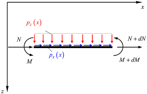
Figure 1. Forces and moments acting on the element.
The bending of the beam is studied in the context of the Euler-Bernoulli beam theory, according to which plane cross-sections of the beam perpendicular to the beam axis before deformation remain (i) plane, (ii) rigid, and (iii) perpendicular to the (deformed) axis after deformation. Following these assumptions, the displacement field is written as.
where (▪),x denotes differentiation with respect to x; are the displacements of an arbitrary point of the beam along the x, y, z axes respectively and u, w are the displacements of a point on the neutral axis.
The components of the three-dimensional Green-Lagrange strain tensor are given (Reddy, 2005a)
Assuming that the strains are small, the terms , εzz, ū,xū,z are negligible compared to u,x (Reddy, 2005a) and substituting the displacement components from Equations (1)–(3) to the strain-displacement relations (4)–(9) the only non-vanishing component of the strain tensor is
Furthermore, the only non-vanishing stress component of the second Piola-Kirchhoff stress tensor is
Governing Equations of the Problem and Boundary Conditions
To establish the equations of equilibrium of the beam, the principle of minimum total potential energy is employed. To this end, the total potential energy of the elastic beam is
where U, V are the strain energy of the beam and the potential of the external forces, respectively. The strain energy per unit volume is given by the integral
and the total strain energy of the beam is
The potential of the external forces applied to the beam is equivalent to the work done on the beam by them
The stress resultants, namely the axial force N and the bending moment M are defined as
According to the principle of minimum total potential energy, the first variation of the total potential energy of the beam must be equal to zero
Substituting Equations (14), (15) in Equation (17) and by virtue of Equations (10), (11), (16) leads to
By applying the Gauss-Green theorem (integration by parts) and collecting the coefficients δu and δw, we obtain
Since δu, δw are arbitrary and independent of each other in the interval (0, l), by virtue of the fundamental lemma of calculus of variations the governing equations become
In case the stress-strain relation is a known function, and analytical integration can be performed on Equation (16), then with respect to Equation (10) the stress resultants in terms of the displacements are written as
Using Equations (22), (23) the governing equations take the form
Examining now the boundary terms of Equation (19), we conclude that (Reddy, 2005b):
• δu, δw, δw,x are the primary variables, and their specification constitutes the essential boundary conditions of the problem.
• N, Nw,x + M,x, M are the secondary variables, and their specification constitutes the natural boundary conditions of the problem.
Among the values comprising the pairs (u, N), (w, Nw,x + M,x), (w,x, M) only one can be prescribed.
Moreover, the boundary conditions of the problem can be written as (Katsikadelis and Tsiatas, 2003)
where ακ, , βκ, , γκ, (κ = 1, 2, 3) are known constants. In Equations (26)–(31) the most general boundary conditions of the problem are described. It is worth noting that they include the case of elastic support of the beam, as well.
Equations (20), (21) in terms of stress resultants or (24), (25) in terms of displacements, along with Equations (26)–(31) constitute the boundary value problem that describes the nonlinear bending of the beam. Analytical solution of the problem is somewhat cumbersome, so a numerical scheme has to be introduced.
Numerical Formulation
The AEM Solution
A direct solution to the boundary value problem described by the coupled Equations (24) and (25) together with the boundary conditions (26)–(31) is achieved on the basis of the AEM formulation for the large deflection analysis of beams of variable stiffness as developed in Katsikadelis and Tsiatas (2003). Briefly discussed, let u = u(x) and w = w(x) be the sought solutions of the problem, having continuous derivatives up to the 2nd and 4th order respectively in (0, L). According to the analog equation principle, the two coupled nonlinear equations can be substituted by the following analog equations
applying the linear differential operators of the second and fourth order respectively to u = u(x) and w = w(x). Both operators have known fundamental solutions. It is noteworthy that Equations (32) and (33) are attributed independently to the linear response of a beam of constant unit stiffness under the fictitious loads b1 and b2 for the axial and bending problem respectively. According to the AEM, the solution of the system of Equations (24) and (25) can be achieved by solving the uncoupled system of Equations (32) and (33) under the same boundary conditions (26)–(31), after the determination of the fictitious load distributions b1, b2. Accordingly, a procedure can be developed by the integral equation method. In this sense, the integral representations of the solutions of Equations (32) and (33) take the following form
where ci (i = 1, 2, …6) are arbitrary integration constants that will be determined from the boundary conditions and
are the fundamental solutions (free space Green's functions) of Equations (32) and (33), respectively.
By direct differentiation of Equations (34) and (35) the derivatives of u and w can be obtained as
Substituting Equations (38)–(43) into Equations (24) and (25) they can be written in terms of the unknown fictitious sources b1and b2.
The next step of the AEM requires the discretization of the domain (0, L) into N elements, not necessarily equal. On each element the variation of each fictitious load b1 and b2 is approximated by a predefined law (constant, linear, parabolic, etc.). In what follows, the elements are considered equal and the constant law is adopted (constant elements).
Subsequently, the integral representation of Equations (34) and (35) can be written in matrix form as
where G1(x) and G2(x) are 1 × N known matrices obtained by integrating the kernels G1(x, ξ) and G2(x, ξ) on the constant elements, respectively; H1(x) = [x 1] and H2(x) = [x3 x2 x 1]; c1 = {c1, c2}T; c2 = {c3, c4, c5, c6}T; b1 b2 are vectors containing unknown fictitious loadings at the N nodes. Likewise, Equations (38)–(43) can be written as
where G1x(x), G2xx(x),… G2xxx(x) are 1 × N known matrices, stemming from the integration of the derivatives of the kernels G1(x, ξ), G2(x, ξ) on the elements; H1x(x) is a 1 × 2 known matrix resulting from the differentiation of H1(x), whereas H2x(x), H2xx(x), H2xxx(x) are 1 × 4 known matrices resulting from the differentiation of H2(x).
The final step of the AEM is the collocation of the Equations (24) and (25) at the N internal nodal points and the substitution of the displacements and their derivatives according to the Equations (44)–(51)
where Fi(b1, b2, c) are generalized stiffness vectors, and . Equations (52) and (53) constitute a system of 2N nonlinear algebraic equations of 2N + 6 unknowns. The additional six equations required to solve the system can be derived from the exploitation of the boundary conditions of the problem. To this end, the related derivatives are substituted into Equations (26)–(31) to give
The nonlinear Equations (52)–(53) in combination with the Equations (54) constitute a system of 2N + 6 algebraic equations with respect to the unknown vectors b1, b2 and c. The solution of the system by any numerical technique provides the values of the fictitious loads at the internal nodal points.
However, when the stress resultants and their derivatives cannot be evaluated analytically, the following layered analysis should be employed.
The Layered Analysis
As a first step to the layered analysis, an appropriate number of monitoring cross-sections is defined along the length of the beam. For convenience purposes, the position of each cross-section coincides with the nodal points of the longitudinal discretization and the two points that correspond to the ends of the beam. Consequently, each cross-section is decomposed into a number of layers of constant height. At the center of each layer, the strain is expressed in terms of the nodal displacement components. Next, given the strain expressions, stresses are computed and employing an appropriate integration scheme, stress resultants are evaluated. The discretization scheme is depicted in Figure 2.
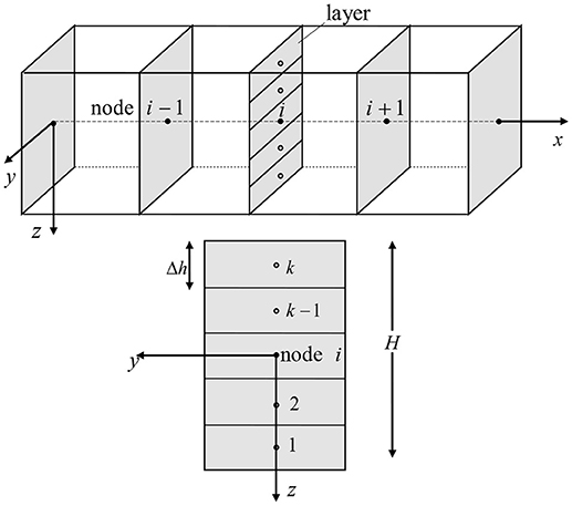
Figure 2. Discretization of the beam into monitoring cross-sections and cross-section layers.
An odd number of layers k is selected so as the center of the beam's cross-section is located at the middle of the (k + 1)/2 layer. The constant height of the layers is Δh. The z coordinate of the center of the i-th layer is written as
The axial force Ni and the bending moment Mi for each layer can be computed as
where are the stress component at the center of each layer and the area of each layer respectively. Therefore, the stress resultants can be approximated as
After evaluating the axial force and the bending moment at each nodal point, their derivatives must be computed to check if the equations of equilibrium hold. To this end, the procedure thoroughly described in Tsiatas and Charalampakis (2017) is adopted.
Having established the numerical expressions of the stress resultants and their derivatives in terms of the unknown fictitious loads, the nonlinear Equations (52)–(54) are solved iteratively. The first iteration starts with an initial guess for the unknown fictitious loads. Next, the displacements and their derivatives are evaluated at all the defined monitoring cross-sections of the beam using the respective integral representations. Subsequently, the stress resultants are computed at each layer using Equations (56), (57) and the whole cross-section by applying Equations (58), (59). Lastly, the governing Equations (20) and (21) are checked for equilibrium. In case the equilibrium is satisfied, the process is terminated. Otherwise, the fictitious load distributions are updated, and the procedure continues with further iterations.
Numerical Examples
Based on the presented numerical procedure, a computer program has been developed, and representative examples have been studied to demonstrate the accuracy and the efficiency of the proposed method of nonlinear analysis.
Example 1: Beam With Fixed Ends Under Concentrated Loading
The first example deals with the geometrical nonlinear static analysis of a fully fixed beam under concentrated loading applied at the midspan. The cross-section of the beam is rectangular b × h and its length is L. The geometrical characteristics of the beam and the cross-section are shown in Figure 3. The beam is made of a linearly elastic material. The employed data for the elastic properties of the material and the geometry of the beam are: E = 2.07 × 10⁸kN/m2, b = 0.0254 m, h = 0.003175 m, and L = 0.508 m.
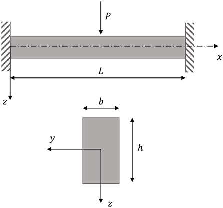
Figure 3. Fixed beam in Example 1.
The present example has been also examined in the studies of Katsikadelis and Tsiatas (2003) and Mondkar and Powell (1977). It is noted that in the study of Katsikadelis and Tsiatas (2003) a BEM scheme for the longitudinal problem is also established, but an analytical procedure to obtain the stress resultants is adopted. Furthermore, Mondkar and Powell (1977) modeled the half of the beam using five eight-node plane stress elements and applied a 2 × 2 Gauss quadrature. Results from both these works are used herein for comparison purposes.
Figures 4A,B show the profiles for the vertical and horizontal displacements respectively, corresponding to load value Pz = 3.11kN. The results of the proposed method are compared with those presented by Katsikadelis and Tsiatas (2003); it can be seen that they are in excellent agreement. In Figure 5, the variation of vertical displacements w at the middle of the beam with respect to the force Pz is presented for the layered approach as well as for both the references above; the identification of the results is noteworthy. In Table 1, deflections at the middle of the beam length are presented for several numbers of longitudinal elements and layers; it can be observed that satisfactory convergence can be achieved for a small number of layers. Finally, Figures 6A–C depict the bending, axial, and shear stress resultants respectively.
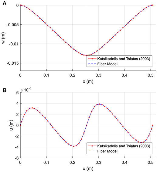
Figure 4. Profiles of the (A) deflection and (B) axial displacement in Example 1.
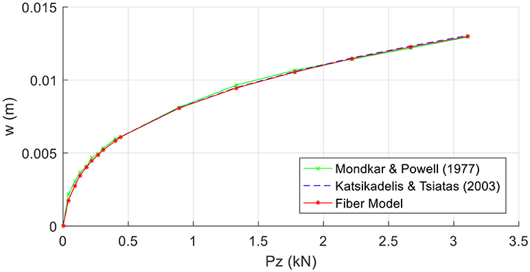
Figure 5. Deflection versus Load at the center of the beam in Example 1.
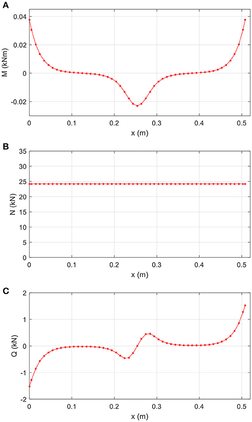
Figure 6. Profile of the (A) bending moment, (B) axial force, and (C) shear force in Example 1.
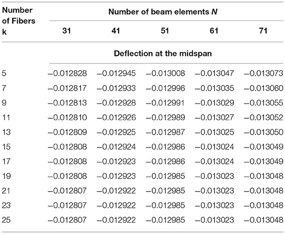
Table 1. Deflection at the midspan in Example 1.
Example 2: Simply Supported Beam Made of Nonlinear Material
For comparison reasons, in the second example an initially straight beam made of a nonlinear elastic material is examined. The cross-section of the beam is rectangular b × h and its length is L. It is pinned at its both ends and is subjected to a uniformly distributed vertical load pz. The employed geometrical data, as shown in Figure 7, is: b = 0.10 m, h = 0.50 m, L = 2.0 m. The constitutive law of the nonlinear elastic material is given by the relation
where σ0 = 410000 kPa, ε0 = 0.017143512. The stress-strain curve is depicted in Figure 8. In this example, the geometrical nonlinear effect is not considered.
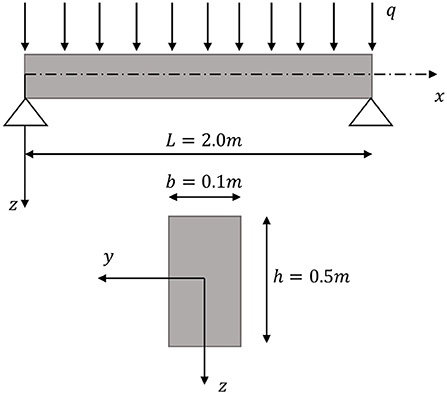
Figure 7. Simply supported beam in Example 2.
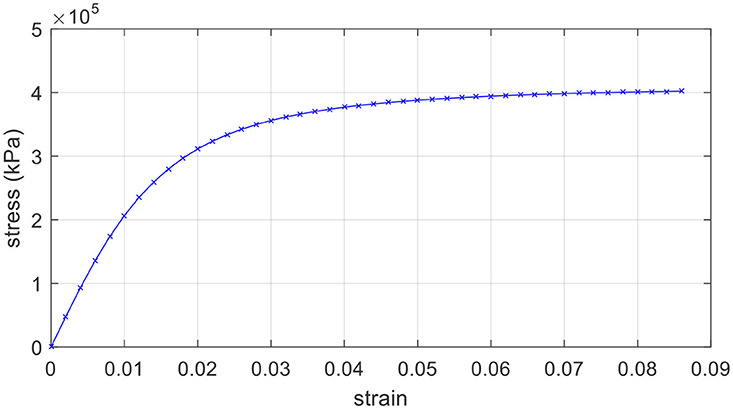
Figure 8. Stress-strain curve for the nonlinear material in Example 2.
In the context of the presented layered methodology, static geometrical linear-material nonlinear analyses are performed for several loading values. The beam length is discretized into 51 elements, and the cross-section is decomposed into 21 layers. The obtained results are compared with corresponding results obtained from two FEM models: (i) a FEM model with 51 beam elements, and (ii) a solid FEM model comprising 12500 hexahedral 8-node elements.
Figure 9 presents the vertical deflections at the middle of the beam versus the vertical load pz. It can be readily observed that the layered model satisfactorily converges to the solid FEM solution, while the beam FEM solution exhibits significant discrepancies for a relatively low value of loading. In Figure 10 the deflection profile for pz = 4541.42kN/m is shown. It is remarkable that the layered analysis yields deflections along the beam that are in excellent agreement with the ones obtained from the solid model.
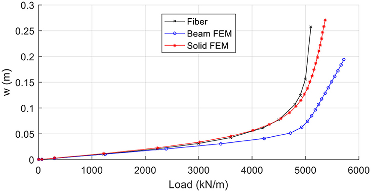
Figure 9. Deflection at the middle of the beam vs. load in Example 2.
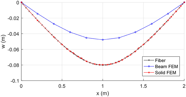
Figure 10. Profile of deflections for pz = 4541.42kN/m in Example 2.
Example 3: Shape Memory Alloy Beam Under Concentrated Loading
In order to demonstrate the range of applications of the proposed methodology of analysis, in this final example, an initially straight clamped beam made of a superelastic Shape Memory Alloy (SMA) is considered. One of the most important mechanical property of SMAs is that they can undergo large inelastic strains recoverable upon load removal (Superelasticity). The SMA's stress-strain relation adopted herein was obtained by interpolating the experimental curve presented in Charalampakis and Tsiatas (2018).
The beam under consideration has a uniform rectangular cross-section b × h, and length L, as shown in Figure 11. It is fixed at its both ends and is subjected to a concentrated vertical load Pz at the middle of its length. The geometrical data is: b = 0.50 m, h = 0.80 m, and L = 1.0 m. The beam is divided into 51 elements along its length, and the cross-section is discretized into 21 layers.
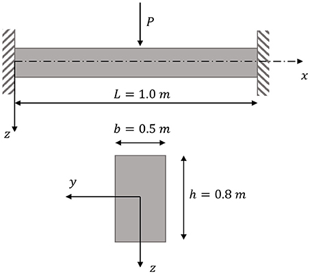
Figure 11. Fixed beam in Example 3.
In this example two cases of analysis are performed, for several loading values: (i) geometrical linear analysis, and (ii) geometrical nonlinear analysis. It is noted that material nonlinearity is taken into account in both cases, and the stress-strain relation is depicted in Figure 12. In Figure 13, the deflections at the midspan vs. the loading variation are presented for both cases of analysis. The effect of geometrical nonlinearity in the decrease of the central deflection for a specific loading range is verified. This effect can also be verified in the comparison of the stress resultants. More specifically, Figure 14A shows the bending moment profiles (Pz = 400kN) where it can be readily observed the decrease of the bending moment, in case of the geometrical nonlinear case, due to the contribution of the axial forces to the loading carriage. Finally, Figure 14B shows the axial force profile (Pz = 400kN) only for the geometrical nonlinear case since in the geometrical linear analysis the axial force is zero.
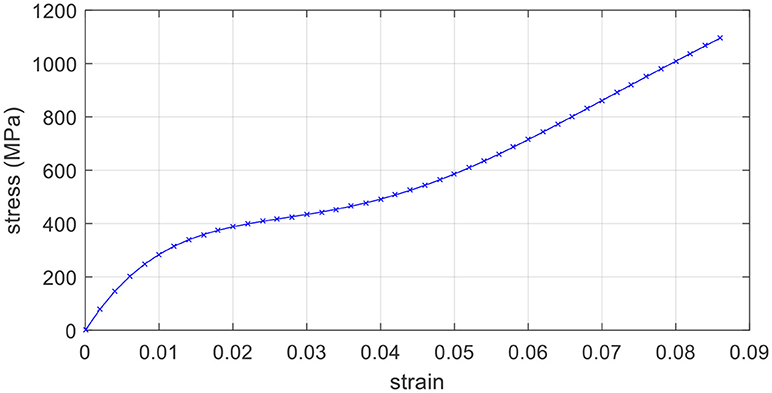
Figure 12. Stress-strain curve for the nonlinear SMA material in Example 3.
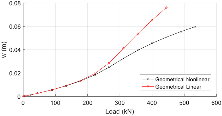
Figure 13. Deflection at the middle of the beam vs. load in Example 3.
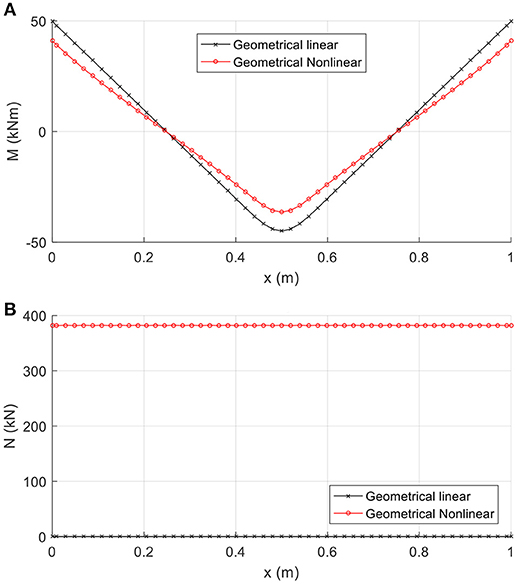
Figure 14. Profile of the (A) bending moment, and (B) axial force, for Pz = 400kN in Example 3.
Conclusions–Future Research
In this work, a layered approach to the nonlinear analysis of beams has been presented. The beam is studied considering both geometrical and material nonlinearity. The governing differential equations were obtained with a variational approach and their system was solved using the AEM in conjunction with an iterative numerical process. To this end, a discretization scheme was established in both the longitudinal sense and the cross-sectional plane. According to the presented analysis and the numerical results, the following main conclusions can be drawn:
a) The layered method has proven to be very competent and together with the AEM can be employed in the solution of difficult nonlinear coupled problems.
b) The method can treat both geometrical and material nonlinearity in a more general context, as compared to existing direct solution methods which are confined only to handling geometrical nonlinearity.
c) The numerical solution is efficient and stable, while a small number of line elements and layers are adequate to achieve significant accuracy for the displacements and the stress resultants.
d) In comparison with the FEM beam model, the layered approach model is capable of giving results that better converge to the ones obtained by a FEM solid model.
e) The proposed layered approach can be easily extended to solve problems of curved beams, as well as beams with arbitrary cross-sections.
f) Furthermore, the limitation of the number of monitoring cross-sections only in locations of high-stress concentration (e.g., beam supports) can be considered as a future application of the layered approach.
Author Contributions
GT had the research idea, contributed to the theoretical analysis, and interpretation of the results. AS drafted the article, and contributed to the derivation of the numerical examples. ES supervised the research. All the authors contributed to the writing of the manuscript.
Conflict of Interest Statement
The authors declare that the research was conducted in the absence of any commercial or financial relationships that could be construed as a potential conflict of interest.
References
Argyris, J. H., Dunne, P. C., Malejannakis, G., and Scharpf, D. W. (1978a). On large displacement - small strain analysis of structures with rotational degrees of freedom. Comput. Methods Appl. Mech. Eng. 15, 99–135. doi: 10.1016/0045-7825(78)90008-7
Argyris, J. H., Dunne, P. C., Malejannakis, G., and Scharpf, D. W. (1978b). On large displacement - small strain analysis of structures with rotational degrees of freedom. Comput. Methods Appl. Mech. Eng. 14, 401–451. doi: 10.1016/0045-7825(78)90076-2
Argyris, J. H., Hilpert, G. A., Malejannakis, G., and Scharpf, D. W. (1979). On the geometrical stiffness of a beam in space. a consistent V. W. approach. Comput. Methods Appl. Mech. Eng. 20, 105–131. doi: 10.1016/0045-7825(79)90061-6
Banerjee, P. K., and Butterfield, R. (1981). Boundary Element Methods in Engineering Sciences. London: Mc Graw - Hill.
Bathe, K. J., and Bolourchi, S. (1979). Large displacement analysis of three-dimensional beam structures. Int. J. Numer Methods Eng. 14, 961–986. doi: 10.1002/nme.1620140703
Becker, A. A. (1992). The Boundary Element Method in Engineering: A Complete Course. New York, NY: Mc Graw - Hill.
Cai, Y., Paik, J. K., and Atluri, S. N. (2009). Large deformation analyses of space - frame structures, with members of arbitrary cross-section, using explicit tangent stiffness matrices, based on a Von Karman type nonlinear theory in rotated reference frames. Comput. Model. Eng. Sci. 53, 117–145. doi: 10.3970/cmes.2009.053.123
Charalampakis, A. E., and Tsiatas, G. C. (2018). A simple rate-independent Uniaxial Shape Memory Alloy (SMA) model. Front. Built Environ. 4:46. doi: 10.3389/fbuil.2018.00046
Filippou, F. C., Taucer, F. F., and Spacone, E. (1991). A Fiber Beam Column Element for Seismic Response Analysis of Reinforced Concrete Structures. EERC Report 91/17, UC Berkeley, Earthquake Engineering Research Center.
Hodges, D. H. (2006). “Progress in astronautics and aeronautics,” in Nonlinear Composite Beam Theory (Reston, VA: AIAA). doi: 10.2514/4.866821
Izzuddin, B. A., Siyam, A. F., and Lloyd Smith, D. (2002). An efficient beam-column formulation for 3D reinforced concrete frames. Comput. Struct. 80, 659–676. doi: 10.1016/S0045-7949(02)00033-0
Kaba, S., and Mahin, S. A. (1984). Refined Modeling of Reinforced Concrete Columns for Seismic Analysis. EERC Report 84/03, UC Berkeley, Earthquake Engineering Research Center.
Katsikadelis, J. T. (2016). The Boundary Element Method for Engineers and Scientists. Oxford: Academic Press, Elsevier.
Katsikadelis, J. T., and Tsiatas, G. C. (2003). Large deflection analysis of beams with variable stiffness. Acta Mech. 164, 1–13. doi: 10.1007/s00707-003-0015-8
Katsikadelis, J. T., and Tsiatas, G. C. (2004). Nonlinear dynamic analysis of beams with variable stiffness. J. Sound Vib. 270, 847–863. doi: 10.1016/S0022-460X(03)00635-7
Mondkar, D. P., and Powell, G. H. (1977). Finite element analysis of nonlinear static and dynamic response. Int. J. Numer. Methods Eng. 11, 499–520. doi: 10.1002/nme.1620110309
Plevris, V., and Tsiatas, G. C. (2018). Computational structural engineering: past achievements and future challenges. Front. Built Environ. 4:21. doi: 10.3389/fbuil.2018.00021
Providakis, C. P., and Beskos, D. E. (1986). Dynamic analysis of beams by the boundary element methods. Comput. Struct. 22, 957–964. doi: 10.1016/0045-7949(86)90155-0
Reddy, J. N. (2005a). An Introduction to Nonlinear Finite Element Analysis. New York, NY: Oxford University Press.
Reddy, J. N. (2005b). An Introduction to the Finite Element Method, 3rd Edn. New York, NY: Mc Graw - Hill.
Sapountzakis, E. J., and Dikaros, I. C. (2011). Nonlinear Flexural-Torsional dynamic analysis of beams of arbitrary cross section by BEM. Int. J. Non Linear Mech. 46, 782–794. doi: 10.1016/j.ijnonlinmec.2011.02.012
Sapountzakis, E. J., and Dourakopoulos, J. A. (2010). Flexural-Torsional nonlinear analysis of Timoshenko beam-column of arbitrary cross section by BEM. Comput. Mater. Continua 18, 121–153. doi: 10.3970/cmc.2010.018.121
Sapountzakis, E. J., and Kampitsis, I. C. (2017). Dynamic analysis of beam-soil interaction systems with material and geometrical nonlinearities. Int. J. Non Linear Mech. 90, 82–89. doi: 10.1016/j.ijnonlinmec.2017.01.007
Sapountzakis, E. J., and Mokos, V. G. (2008). Shear deformation effect in nonlinear analysis of spatial beams. Eng. Struct. 30, 653–663. doi: 10.1016/j.engstruct.2007.05.004
Sapountzakis, E. J., and Panagos, D. G. (2008). Nonlinear analysis of beams of variable cross section including shear deformation effect. Arch. Appl. Mech. 78, 687–710. doi: 10.1007/s00419-007-0182-5
Taylor, G. A. (1996). A Vertex Based Discretization Scheme Applied to Material Non-Linearity Within a Multiphysics Finite Volume Framework. London: University of Greenwich.
Tsiatas, G. C. (2010). Nonlinear analysis of non-uniform beams on nonlinear elastic foundation. Acta Mech. 209, 141–152. doi: 10.1007/s00707-009-0174-3
Tsiatas, G. C., and Charalampakis, A. E. (2017). Optimizing the natural frequencies of axially functionally graded beams and arches. Composite Struct. 160, 256–266. doi: 10.1016/j.compstruct.2016.10.057
Tsiatas, G. C., Siokas, A. G., and Sapountzakis, E. J. (2018). “A fiber approach to the large deflections analysis of beams by BEM,” in 9th GRACM, International Congress on Computational Mechanics (Chania).
Yang, Y., and McGuire, W. (1986). Stiffness matrix for geometric nonlinear analysis. J. Struct. Eng. ASCE 112, 853–877. doi: 10.1061/(ASCE)0733-9445(1986)112:4(853)
Keywords: beams, geometrical nonlinear analysis, material nonlinear analysis, Boundary Element Method (BEM), layered analysis, shape memory alloys (SMA)
Citation: Tsiatas GC, Siokas AG and Sapountzakis EJ (2018) A Layered Boundary Element Nonlinear Analysis of Beams. Front. Built Environ. 4:52. doi: 10.3389/fbuil.2018.00052
Received: 11 July 2018; Accepted: 04 September 2018;
Published: 09 October 2018.
Edited by:
Raffaele Barretta, Università degli Studi di Napoli Federico II, ItalyReviewed by:
S. Ali Faghidian, Islamic Azad University, IranGiovanni Romano, Università degli Studi di Napoli Federico II, Italy
Copyright © 2018 Tsiatas, Siokas and Sapountzakis. This is an open-access article distributed under the terms of the Creative Commons Attribution License (CC BY). The use, distribution or reproduction in other forums is permitted, provided the original author(s) and the copyright owner(s) are credited and that the original publication in this journal is cited, in accordance with accepted academic practice. No use, distribution or reproduction is permitted which does not comply with these terms.
*Correspondence: George C. Tsiatas, Z3RzaWF0YXNAdXBhdHJhcy5ncg==