 Mohammad Miralinaghi
 Srinivas Peeta
- Lyles School of Civil Engineering/NEXTRANS Center, Purdue University, West Lafayette, IN, United States
This study focuses on a tradable credit scheme (TCS)-based multi-period equilibrium modeling framework to address the planning problem of a central authority which seeks to minimize the vehicular emissions in a traffic network over a planning horizon. In this context, the multi-period TCS equilibrium conditions consist of traffic, and market equilibrium conditions. To develop an effective TCS design in practice, this study factors the heterogeneity in travelers' value of time (VOT) to enable realism in capturing the traffic equilibrium conditions, and the interest rate to reflect market realism. The VOT is an important factor in the route choice process as travelers tradeoff the credit consumption and travel time costs of each route. Further, travelers decide between selling or transferring unused credits across periods based on the dynamic interest rates over the planning horizon as they can accrue interest by selling credits in the market. The study investigates the existence and uniqueness of multi-period equilibrium credit prices, aggregate link flows and travel demand rates. Then, the equilibrium credit prices under the multi-period TCS are analyzed and it is demonstrated that while credit price volatility increases with increasing interest rates, it can be dampened by the ability of travelers to transfer credits under the multi-period TCS. Finally, a system optimal (SO) multi-period TCS is designed to determine the TCS parameters (credit allocation and charging schemes) that minimize vehicular emissions in a traffic network over the planning horizon. The study insights suggest that the SO design of multi-period TCS provides a capability to manage network vehicular emissions over the planning horizon. Further, they suggest that if VOT is not factored, the TCS would be socially inequitable, and ignoring interest rates creates inefficiencies in achieving desired emissions levels.
Introduction
Over the past few decades, human impact on the climate has been correlated to greenhouse gas (GHG) emissions produced by human activities such as those related to the use of fossil fuels. To address this issue, there are worldwide efforts to reduce GHG emissions in different sectors. For example, the European Union has targeted at least a 40% reduction of GHG emissions by 2,030. The transportation sector contributes significantly to global GHG emissions; it accounted for ~26% of the total U.S. GHG emissions in 2014 (U. S. Environmental Protection Agency, 2016). Vehicular traffic contributes significantly to the levels of carbon monoxide (CO), nitrogen oxide (NOx), carbon dioxide (CO2), particulate matter (PM), and hydrocarbons (HC). Because of its negative effect on living and health conditions in metropolitan areas, transportation planners (referred to as “central authority (CA)” in this study) have focused on strategies to reduce GHG emissions of traffic congestion. In this context, market-based instruments can be leveraged to develop efficient strategies to manage travel demand and reduce harmful GHG emissions in metropolitan areas.
Road pricing is the most well-known market instrument to tackle traffic externalities in metropolitan areas. Congestion, pollution and noise are examples of externalities in the traffic network. Pigou (1920) developed the notion of marginal cost pricing in which the travelers are charged the external cost (as toll) that they impose on each other in the traffic network. It influences the travel choices of travelers so as to reduce traffic externalities. Studies thereafter have sought to develop the underlying economic model of road pricing (Vickrey, 1969; Yang and Huang, 2005) by focusing on the traffic congestion externality. In the context of addressing the emissions externality, Johansson (1997) employs the notion of marginal cost pricing to maximize net social benefit where travelers are charged for their emissions and the increase in the emissions of other travelers. Yin and Lawphongpanich (2006) design a pricing strategy to internalize the emissions externality in the traffic network which yields a traffic flow distribution with minimum emissions.
Although road pricing is appealing in theory, it has been sparsely implemented in practice for two reasons. First, travelers perceive toll as an indirect tax imposed by the CA. Second, it increases the potential for inequity across road users as low-income travelers are disproportionately forced to change their travel habits. To overcome these two issues, Lawphongpanich and Yin (2010) develop a class of Pareto-improving pricing scheme in which no traveler is worse off compared to the no-pricing scheme. However, even this scheme cannot preclude the transfer of wealth from the travelers to the CA.
To address issues with congestion pricing, quantity-based instruments have been proposed to increase public acceptance and address the negative traffic externalities. They have been applied in different sectors to control air quality, water pollution and land use (Tietenberg, 2004). The most well-known implementation of quantity-based instruments is the European Union (EU) Emissions Trading System (ETS) with the objective of reducing CO2 emissions, as a type of GHG emissions, to at least 80% of the 2005 emissions level by 2,050. In the EU ETS, the European power plants, factories and other companies receive a predetermined number of pollution permits by the EU. They are subject to a predetermined emissions cap and are able to trade CO2 pollution permits in the market to meet a predetermined emissions cap (Ellerman and Joskow, 2008). Quantity-based instruments have been analyzed for controlling congestion and emissions in traffic networks. Verhoef et al. (1997) investigate the use of a tradable permit scheme to manage externalities by allowing travelers to pay tolls using smart cards as well as to trade the units stored in them. This idea is further examined by Viegas (2001) to mitigate traffic congestion. Nagurney et al. (1998) propose the notion of link-based pollution permits to minimize total vehicular emissions where each link is initially allocated a certain number of permits. In other words, there is a cap on the total number of vehicles that can traverse each link.
Along this thread, a tradable credit scheme (TCS) is a strategy to achieve different system-level goals of CA such as mitigating congestion or vehicular emissions, by creating artificial markets for mobility credits. In this scheme, the CA allocates credits free of cost to travelers who then pay credits to use their vehicles on a link. Such a scheme can also foster travelers to consider less-expensive public transit systems. Further, under TCS, travelers can trade credits amongst themselves in the market. Two types of equilibrium conditions exist in the traffic network under TCS, including: (i) traffic equilibrium condition, under which travelers cannot reduce their travel costs by unilaterally switching routes, and (ii) market equilibrium condition, under which the equilibrium credit price (ECP) is positive only if there are no unused credits in the market. There is potentially less societal objection to TCS implementation in practice, for two reasons. First, there is no transfer of wealth from travelers to the CA. Second, TCS is a more equitable strategy compared to congestion pricing as low-income travelers, who typically choose less-expensive travel options, can sell unused credits and gain monetary benefits.
Yang and Wang (2011) propose a TCS to address the traffic congestion externality. It is formulated within the static user equilibrium framework and includes a credit conservation constraint. Wang et al. (2012) further consider travelers' heterogeneity in terms of value of time (VOT) in analyzing the equilibrium condition under TCS. Zhu et al. (2015) address VOT heterogeneity by adopting a continuous distribution of VOTs across travelers. Bao et al. (2014) study the effects of travelers' loss aversion behavior on their route choice decisions under TCS, where purchasing extra credits is perceived as monetary loss. Other studies deal with: (i) the assumptions of a competitive market (Nie, 2012; Shirmohammadi et al., 2013), and (ii) capturing traffic dynamics under TCS (He et al., 2013; Xiao et al., 2013). The CA's objective in the aforementioned TCS studies is to minimize the total system travel cost by using the total number of credit endowments and the subsequent link-based credit charges as control parameters. Aziz and Ukkusuri (2013) seek to address the vehicular emissions externality through SO TCS design by deriving credit allocation and charging schemes for homogeneous travelers. Miralinaghi and Peeta (2016) label the aforementioned TCS models as “single-period TCS.” In a single-period TCS, it is assumed that the traffic network supply (for example, the link travel cost functions) and travel demand functions are time-invariant during the planning horizon. Hence, the single-period TCS is not an appropriate tool to achieve long-term planning goals, such as addressing traffic congestion and emissions externalities, as it cannot capture demand and/or supply fluctuations over the planning horizon (in the order of a few years).
Miralinaghi and Peeta (2016) propose a framework, labeled “multi-period TCS” for the planning context which enables the CA to design a multi-period TCS by factoring the long-term fluctuations in travel demand and/or traffic network supply. In this framework, the planning horizon is divided into multiple periods of equal length. In each period, the CA allocates credits to travelers at a predetermined rate based on the credit allocation scheme. For each period, it also predetermines the credit rate charged per link, labeled the credit charging scheme. The credit allocation and charging schemes are referred to as “TCS parameters” hereafter. Travelers consume or transfer unused credits in the current period based on different factors, e.g., projected credit prices in future periods, current travel demand, current TCS parameters, and current traffic network supply. Hence, unlike in single-period TCS, the traffic and market equilibrium conditions under multi-period TCS depend on the projected credit prices of future periods. The multi-period TCS framework enables the CA to assess the progress toward long-term goals at the end of each period. Then, the CA adjusts the TCS parameters for future periods based on the current progress toward system-level goals and updated forecasts of future travel demands. Further, the multi-period TCS allows the CA to tradeoff credit price volatility across periods with the need to achieve long-term goals (for example, traffic network emissions over the planning horizon). Finally, a multi-period TCS can foster gradual progress toward goals (such as, reductions in vehicular emissions), enabling travelers to better adjust to the TCS in practice. For example, the EU has sought to gradually reduce the emissions cap from 97% average of the 2005 values in 2012 to 95% in 2020, and 80% in 2050 (Leggett et al., 2012). This enables European companies to better adapt to the EU ETS by investing in more efficient technologies to meet their reduced emissions caps in future years.
This study focuses on managing traffic network emissions over a long-term planning horizon in the order of several years. To do so, we seek to develop the system optimal (SO) TCS to obtain the TCS parameters (credit allocation and charging schemes) that minimize vehicular emissions over that horizon. Similar to the EU ETS, the CA should design the SO TCS so that travelers would be able to better adapt to the TCS over the planning horizon by changing locational and/or mode choices. For example, low-income travelers often choose residential locations that require longer distances to reach their workplaces (Aziz and Ukkusuri, 2013). If their travel costs increase abruptly after a TCS implementation, it can be perceived as inequitable and is not sustainable in practice. Further, travelers may change their home locations during the planning horizon to have greater accessibility to public transit to avoid paying credits. Hence, this study aims to develop a SO design of the multi-period TCS so that travelers can gradually adapt to the TCS over the planning horizon. In this context, as the goal of the CA is to minimize total vehicular emissions, the SO TCS design can entail low credit supply and high credit charges for usage of transportation facilities. This can significantly increase credit consumption costs across periods, and the travel cost of travelers because it includes credit consumption costs in addition to travel time costs. Such significant cost increases in consecutive periods is not sustainable from travelers' perspective, implying the need to bound travel cost increases across periods. To address this issue, we bound the travel cost of each user class for each O-D pair in the first period, and further bound cost increases in subsequent periods. This enables travelers to better adjust to the TCS implementation in practice.
To achieve an effective, sustainable SO multi-period TCS design, this study incorporates the VOT heterogeneity of travelers to foster realism in the traffic equilibrium condition, and interest rate to more realistically capture the market equilibrium condition. VOT reflects how travelers view travel time savings. In the route choice process, travelers tradeoff credit consumption and travel time costs using VOT. Interest rate is defined as the rate at which capital grows (Thuesen and Fabrycky, 2001). Due to the long-term nature of a multi-period TCS, interest rates are an inevitable factor in traveler decisions related to transferring credits to future periods as credits have monetary value. Interest rates are determined by several factors such as the risk of monetary loss, inflation, and opportunities for investing money with various outcomes over the long-term planning horizon. Besides transferring credits to future periods, travelers also have the option to sell credits and use earned cash toward purchasing credits in future periods while receiving interest on unspent cash. There are several ways to earn interest on capital raised by selling credits in the market. Depositing money in banks is the most common approach. In this study, the interest rate can vary during the planning horizon. Further, it is assumed that the CA uses forecasted bank interest rates as the benchmark of capital growth to determine TCS parameters through the planning horizon.
Miralinaghi and Peeta (2016) focus on analyzing the impact of the multi-period TCS on the evolution of the ECP through the planning horizon. They show that it reduces fluctuations in the ECP through the planning horizon. However, they assume the multi-period TCS is known a priori to the CA and is not necessarily SO as it is not focused on a specific goal. That is, in contrast to the current study, they do not determine the SO multi-period TCS design to reduce vehicular emissions through the planning horizon. Further, they do not consider the effects of travelers' VOT heterogeneity and interest rate. In this study, travelers are divided into multiple discrete user classes, where the average VOT of each user class is used to determine the travel cost of each path for that class. The VOT of each user class is assumed to vary across periods but is unchanged within a period. If VOT is not factored, the SO multi-period TCS design can lead to high travel costs for travelers with lower VOT. Consequently, it can be perceived as a socially inequitable policy in practice since low-income travelers often have lower VOT. When interest rate is ignored, Miralinaghi and Peeta (2016) show that credit price decreases monotonically over the planning horizon. However, this may not be realistic in practice due to several factors such as demand uncertainty, future credit price uncertainty, and market factors such as interest rate. Further, as shown through the numerical experiments in the current study, an SO multi-period TCS design that does not factor interest rate can lead to less-effective schemes to minimize vehicular emissions over the planning horizon.
This study contributes to the literature in five ways. First, it investigates equilibrium conditions under a given multi-period TCS by factoring interest rate and travelers' VOT heterogeneity. This enhances practical realism and enables the CA to better forecast the market and traveler behavior in practice. Second, it demonstrates the solution existence and uniqueness of ECP, equilibrium link flows, and travel demand rates. Uniqueness of credit price is a sign of a healthy market; otherwise, travelers would have to purchase credits with price uncertainty which can reduce travel choices as credit price increases (Miralinaghi et al., 2017). Third, it is proved that if travelers can transfer credits in a multi-period TCS, then credit price volatility reduces through the planning horizon. The stability of credit price would enhance public acceptance of a multi-period TCS because travelers can hedge against potential monetary losses associated with trading credits. Fourth, this is the first study to address the long-term emissions goal for a CA through the design of a SO TCS in terms of the TCS parameters. The proposed SO design also enables the CA to determine the trajectory of the vehicular emissions during the planning horizon given the forecast of future travel demand and traffic network supply. Fifth, the study provides key insights on the roles of interest rates and travelers' VOT heterogeneity in multi-period TCS design. Ignoring travelers' VOT heterogeneity in the SO multi-period TCS can lead to socially inequitable strategies which increase the travel costs of travelers with lower VOT. Further, if interest rate is not factored, the SO multi-period TCS design can lead to less-effective schemes to reduce vehicular emissions.
As this study focuses on the planning context of the multi-period TCS framework, it has two assumptions. First, travelers know the forecasted credit price for each period at the beginning of the planning horizon; these prices are forecasted by solving the planning problem a priori. Second, travelers know the bank interest rate for each period of the planning horizon. These assumptions would need to be addressed in an operational context through a rolling horizon approach that would factor more robust estimates for future periods as time progresses. Further, the TCS design entails the following specific assumptions. The transaction cost in the market is assumed to be negligible and is ignored in this study. Travelers are not charged for transferring credits to future periods. At the end of the planning horizon, unused credits expire without gainful value.
The remainder of the paper is organized as follows. In section 2, some notation is introduced and the TCS types are discussed. In section 3, the equilibrium condition is proposed under VOT heterogeneity and interest rate consideration for multi-period TCS. The existence and uniqueness of the equilibrium aggregate link flows, traffic network demand rates and credit price are investigated under the multi-period TCS. In section 4, the evolution of ECPs under multi-period TCS and multi single-period TCS are compared. In section 5, with factoring the interest rate and VOT heterogeneity, the SO design of multi-period TCS is obtained to minimize the vehicular emissions in a traffic network over the planning horizon. In section 6, the results of some numerical experiments are discussed. Section 7 provides concluding comments.
Preliminaries
Network
Define G(N, A) as a general traffic network where N and A denote the set of nodes and links, respectively. Let t be a time period in the planning horizon where Γ denotes the set of periods with cardinality of T. Let W denote the set of O-D pairs. Travelers are divided into discrete classes based on the VOT. Let M be the set of such user classes where the average VOT of travelers of each user class m ∈ M in each period t ∈ Γ is represented by βm,t. The travel demand and traffic network supply are assumed to be constant within each period. That is, within day or day-to-day fluctuations of traffic conditions in each period are ignored due to the planning context. The interactions between travel demand and credit supply are analyzed per unit of time (for example, an hour). The travel demand rate of user class m for O-D pair w is denoted by and is assumed to be a function of the minimum travel cost of user class m for O-D pair w in time period t. Let Rw denote the feasible route set for O-D pair w ∈ W. The relationship between flow of user class m on link a, aggregate link flow , and flow of user class m on route r of O-D pair w in period t, , can be expressed as follows:
where δa,r,w = 1, if link a is on route r of O-D pair w, and 0 otherwise. The travel cost of each class on each route includes the monetized cost of route travel time (travel time is transferred into equivalent monetary value using VOT) and the charged credit cost of that route. Let be the inverse demand function which is continuous and strictly decreasing in .
We denote the travel demand rates, route flows and link flows in vectors as , , and . Let Ω represent the feasible set of travel demand rates, route flows, and link flows, defined by:
For simplicity, the link travel time function for each link a ∈ A in period t is assumed to be nonnegative, separable, differentiable, and monotonically increasing with link flow in period t. The link travel time functions are assumed to be strictly weighted average monotone over a given set of VOT for each period t. In other words, for any and , ().
Types of Tradable Credit Schemes
single-period TCS studies focus on the equilibrium state of a traffic network in which demand and supply are assumed to be constant during the planning horizon. The credit price under the single-period TCS is referred to as the “single-period credit price” and its equilibrium state is referred to as the “single-period ECP.” In a multi-period TCS, the CA divides the planning horizon into multiple time periods such that the time required to reach the equilibrium state in each period is small compared to its length. Further, travel demand and traffic network supply are assumed constant within each period. Then, the equilibrium link/route flows and credit price for each period represent the traffic and market steady-state conditions. Under the multi-period TCS, the credit price in a period is labeled the “multi-period credit price” and its equilibrium value is referred to as the “multi-period ECP.”
Miralinaghi and Peeta (2016) investigate another scheme, called the “multi single-period TCS”, in which the CA regulates unused credits at the end of each period so that they are discarded without any gainful value. Thereby, travelers are only able to consume or sell credits in each period. The multi single-period TCS is a special case of the multi-period TCS in which travelers do not transfer credits across periods. Because the equilibrium condition in each period can be analyzed independently without considering transferred credits from other periods, the credit price in each period is identical to its single-period credit price and its equilibrium is identical to the single-period ECP.
Equilibrium Condition Under Multi-Period TCS
Model Formulation
The CA distributes credits among travelers at the rate of ξt in period t which is the average number of issued credits per unit of time. The credit allocation scheme consists of credits distributed equally among the travelers. Let denote the class-agnostic link-based credit charging scheme in period t, where denotes the number of credits that travelers pay to use link a at any time in period t. Travelers transfer unused credits in a period t′ at the rate of zt′,t to a period t > t′ without penalty, where z = {zt′,t, ∀t′, ∀t > t′} denotes the vector of the rates of credit transfer. Unused credits are discarded in the last period T at the rate of YT.
Let pt denote the multi-period credit price in period t and pt* denote the multi-period ECP in that period. p* = {pt*, ∀t} represents the vector of multi-period ECPs. The interest rate st,t+1, at which the invested cash in the bank compounds from each period t to the next period t + 1, is assumed to be positive. If travelers sell unused credits in a period t′ and deposit their monetary value in the bank, the sum of initial investment and compounded interest in period t is:
where σt′,t denotes the future monetary value of a credit from period t′ in period t, and αt′,t is the ratio of future value of bank deposits of period t′ in period t to that of its present value. αt′,t is labeled the ratio of future value to present value (RFP) in the rest of this study. σt′,t* is the future monetary value of a credit from period t′ under the equilibrium condition (which is the multi-period ECP of period t′) in period t. Let (fM*,νM*, ν*, dM*, p*, z*,YT*) be the vector of multi-period equilibrium route flows, link flows, aggregate link flows, travel demand rates, credit prices, credit transfer rates, and rate at which unused credits are discarded in the last period. The multi-period equilibrium problem can be formulated as a mathematical program with complementarity constraints (MPCC):
where is the minimum travel cost of user class m for O-D pair w. Mathematical operator ⊥ means that vectors x⊥y if and only if xTy = 0. Complementarity constraints [(5)-(7)] denote the traffic equilibrium condition. Constraint (5) states that for each time period t, the travel costs of all utilized routes for O-D pair w by travelers of class m are equal to . Constraint (6) states that if the travel demand of user class m for O-D pair w is greater than zero, then the inverse demand function is equal to the minimum travel cost of user class m for O-D pair w. Constraint (7) ensures the feasibility of travel demand rates, route flows and link flows. Constraints (8)-(12) represent market equilibrium condition. Constraint (8) states that the sum of credit transfer rates to future periods and credit consumption rate in the first period is equal to the issued credit rate in the first period. Constraint (9) states that the credit supply rate in each period, including credit transfer rates from previous periods and issued credits rate, is equal to the sum of credit consumption rate and credit transfer rates to future periods. Constraint (10) states that the sum of credit consumption rate and rate at which credits are discarded by travelers in the last period is equal to its credit supply rate. Constraint (11) states that the future monetary value of a credit from period t′ in period t is higher than the multi-period ECP of period t. Further, it states that if unused credits are transferred from period t′ to a future period t > t′, the future monetary value of a credit from period t′ in period t is equal to the multi-period ECP of period t. Credits are transferred from period t′ to a future period t with higher single-period ECP until the future monetary value of a credit from period t′ in period t is equal to the multi-period ECP of period t. Hence, the total monetary value of credits is preserved after transferring credits to period t. If travelers continue to transfer additional credits from period t′ beyond the equilibrium point, they tolerate monetary loss. Hence, travelers cannot benefit by unilaterally storing such additional credits under the equilibrium condition. Constraint (12) states that if credits are discarded in the last period T, the multi-period ECP of period T is equal to zero. It also ensures that unused credits are discarded at the end of the planning horizon without benefit for travelers. Next, the existence and uniqueness of solutions of MPCC (5)-(12), in terms of multi-period equilibrium aggregate link flows, travel demand rates and credit prices, are investigated using variational inequality (VI).
Model Properties: Solution Existence and Uniqueness
It is important to investigate the uniqueness of multi-period ECP as it signifies a healthy market. Otherwise, travelers will have to purchase credits at uncertain prices, which can reduce their travel choices as the multi-period ECP increases. To do so, we start by exploring the solution existence of MPCC (5)–(12) by formulating it as a VI problem. Then, sufficient conditions are established for the uniqueness of multi-period equilibrium aggregate link flows and travel demand rates. Finally, the sufficient conditions for uniqueness of multi-period ECP are established. To illustrate the solution existence of MPCC (5)–(12), it is reformulated as VI problem (13)–(17) which is proved to have a solution.
Proposition 1. The following VI problem (13) is equivalent to MPCC (5)–(12).
Proof. (fM*, νM*, ν*, dM*, p*, z*, YT*) solves the VI problem (13)–(17) if and only if it solves the following linear optimization problem:
(14)–(17).
Let γ = {γt, ∀t} denote the set of Lagrangian multipliers of the credit conservation constraints (14)–(16). The first order conditions (Karush-Kuhn-Tucker (KKT) conditions) are:
where is the set of Lagrange multipliers associated with flow conservation constraint (17). A comparison of KKT conditions (19)-(26) with MPCC (5)-(12) illustrates that Lagrangian multipliers γ are equal to the multi-period ECPs p*. Hence, the solution (fM*,νM*, ν*,dM*, p*, z*,YT*) of VI problem (13)-(17) is identical to the solution of MPCC (5)-(12). ■
Proposition 2. The VI problem (13)-(17) admits at least one solution.
Proof. The feasible solution space of VI problem is compact and convex. Further, , and (αt′,t − 1)pt′* are continuous with respect to the route flows, aggregate link flows, travel demand rates, multi-period ECPs, and credit transfer rates. Then, according to Facchinei and Pang (2003), there exists at least one solution (fM*,νM*, ν*,dM*, p*, z*,YT*) to VI problem (13)-(17). ■
Proposition 2 illustrates that there exists a solution (fM*, νM*, ν*, dM*, p*, z*, YT*) to MPCC (5)-(12). Next, a sufficient condition is constructed for the uniqueness of the multi-period equilibrium link flows and travel demand rates (ν*, dM*).
Since the credit charging scheme is known and constant, the uniqueness of multi-period equilibrium link flows leads to the uniqueness of credit consumption rate in each period under the equilibrium condition. Let Δt denote the net credit transfer rate of period t which is given by:
By using Constraint (15), Equation (27) can be re-written as:
The net credit transfer rate in each period is equal to the consumption rate of transferred credits in that period. If the credit consumption rate is higher than the issued credit rate in each period (Δt > 0), it implies that travelers consume transferred credits in addition to issued credits in that period. If the credit consumption rate is unique, then the net credit transfer rate is unique under the equilibrium condition. However, the credit transfer rates z may not be unique as discussed by Miralinaghi and Peeta (2016). The next proposition investigates the uniqueness of the multi-period equilibrium link flow pattern ν*.
Proposition 3. If the multi-period ECPs are unique, then the multi-period equilibrium travel demand rates and link flows are unique.
Proof. Let p* = {pt*, ∀t} denote the vector of the multi-period ECPs through the planning horizon. Then, MPCC (5)-(12) can be reformulated as following nonlinear optimization problem:
It can be verified that for any given p*, (ν*,dM* ) solves nonlinear optimization problem (29)-(30). Because of the assumed properties of the link travel time and inverse demand functions, the objective function is convex in terms of the aggregate link flows and travel demand rates. Hence, MPCC (5)-(12) yields unique multi-period equilibrium travel demand rates and link flows. ■
Proposition 3 proves that the uniqueness of the multi-period ECPs is a sufficient condition for the uniqueness of the multi-period equilibrium travel demand rates and link flows. Miralinaghi and Peeta (2016) show that the multi-period ECP in period t is unique if it satisfies at least one of the following conditions: (i) There exist at least two equilibrium routes connecting one O-D pair with the same travel cost and different credit charges, (ii) Credits are transferred from a previous period with unique multi-period ECP to period t, and (iii) Credits are transferred from period t to a future period with unique multi-period ECP. Hence, the linkage of multi-period ECPs across periods increases the possibility of uniqueness of multi-period ECPs. Similarly, the next proposition establishes the uniqueness conditions for multi-period ECPs under traveler VOT heterogeneity.
Proposition 4. The multi-period ECP in period t is unique if at least one of the following conditions is satisfied:
1. The multi-period equilibrium aggregate link flows ν* are unique and there exist at least two equilibrium routes connecting one O-D pair with the same travel cost and different credit charges for at least one user class in period t.
2. Credits are transferred from a previous period with unique multi-period ECP to period t.
3. Credits are transferred from period t to a future period with unique multi-period ECP.
Proof. The proof follows the similar approach to Wang et al. (2012) and Miralinaghi and Peeta (2016). ■
As discussed in Miralinaghi and Peeta (2016), the multi-period TCS leads to the linkage of multi-period ECPs throughout the planning horizon; this increases the possibility of unique multi-period ECPs.
4. Travelers and market behaviors under multi-period TCS.
In this section, travelers' and market behaviors are compared under the multi single-period TCS and multi-period TCS. As discussed earlier, the multi single-period TCS is a special case of the multi-period TCS in which the credit transfer rates z are equal to zero. Hence, there is no linkage between the multi-period ECPs across periods. If credit transfer rates z in MPCC (5)-(12) are set to zero, the multi-period ECPs are equal to the single-period ECPs. Because constraint (11) is satisfied with zero credit transfer rates, the multi-period ECP can increase or decrease during the planning horizon. The next proposition investigates the effect of interest rate on the evolution of multi-period ECPs during the planning horizon.
Proposition 5. If credits are transferred from period t′ to a future period t given a positive interest rate, then the multi-period ECP of period t′ is lower than the multi-period ECP of period t.
Proof. Constraint (11) implies that if credits are transferred from period t′ to period t, it follows that:
Since interest rate is positive, then αt′,t > 1, and it follows that:
Hence, the multi-period ECP of period t′ is less than the multi-period ECP in period t. ■
Proposition 5 has an important interpretation. As discussed earlier, travelers can transfer unused credits in the current period t′ to consume/sell in any future period t. As a special case of the multi-period TCS with interest rate, Miralinaghi and Peeta (2016) demonstrate that if interest rate is equal to zero, then the multi-period ECP declines during the planning horizon. However, the realized market credit price may not decrease in practice over the planning horizon because of several factors such as interest rate. Proposition 5 illustrates that interest rate is one of the factors that prevents the multi-period ECP from monotonically decreasing over the planning horizon. Under a positive interest rate, travelers accrue interest by depositing the monetary value of sold credits in the bank. Under the equilibrium condition, travelers are indifferent between selling unused credits in the current period t′ or a future period t. Hence, the future multi-period ECP pt* is strictly greater than that of the current period pt′* if travelers transfer credits from period t′ to period t under a positive interest rate. It indicates that the multi-period ECP can increase or decrease during the planning horizon under a positive interest rate. Hence, to address the CA's emissions goals, it is necessary to factor interest rate and travelers' ability to earn interest by selling credits as they affect the multi-period ECPs, and consequently route choices and travel demand rates. The next proposition analyzes the difference between the single-period ECP and multi-period ECP in each period when travelers can transfer credits to future periods under the multi-period TCS.
Proposition 6. Credits are transferred from period t′ (Δt′ < 0) to potentially consume in period t (Δt > 0) only if the single-period ECP of period t′ is lower than the single-period ECP of period t.
Proof. Suppose credits are transferred from time period t′ for possible consumption in a period t. According to Proposition 5, the multi-period ECP in period t is higher than the multi-period ECP in period t′. So, it is sufficient to prove the following two points: (i) the single-period ECP is higher than the multi-period ECP in period t, and (ii) the single-period ECP is lower than the multi-period ECP in period t′. To prove the first point, let be the equilibrium link flows and travel demand rates under the single-period TCS. Wang et al. (2012) formulate the single-period TCS as the following optimization problem:
Constraint (34) states that travelers either consume or discard credits in period t under the single-period TCS. Given the single-period ECP , the optimization problem (33)-(35) is as follows:
Because the single-period equilibrium link flows and travel demand rates are the optimal solution, the optimal value of the objective function can be obtained as:
If travelers consume transferred credits at the net rate of Δt under the equilibrium condition in future period t under the multi-period TCS, the optimization problem for multi-period TCS in period t can be formulated as follows:
Constraint (40) states that travelers either consume or transfer credits to future periods under the multi-period TCS. Since the credit consumption rate of travelers is higher under the multi-period TCS compared to the single-period TCS, it follows that the equilibrium link flows and travel demand rates under the multi-period TCS (ν*, d*) are different than those under the single-period TCS, . Since travelers either consume or discard transferred credits in the last period T, the net credit transfer rate of period T, expressed in Equation (27), can be re-written as follows:
where ψt, T and φt, T denote the rates of consumption and discarding, respectively, of the transferred credits from period t in period T. Let . By combining with constraint (42), constraint (40) can be re-written as follows:
Using equality (43), the optimization problem (39)-(41) for the multi-period TCS can be reformulated as:
Given the multi-period ECP pt*, the optimization problem (44)-(46) can be re-written as:
As the multi-period equilibrium link flows and travel demand rates (ν*,dM*) are the optimal solution, the optimal value of the objective function can be obtained as:
Although the multi-period equilibrium link flows and travel demand rates (ν*, dM*) are feasible solutions for the optimization problem (36)-(37), they are not the optimal solution. Substituting (ν*, dM*) into objective function (36), it follows that:
Further, if the single-period equilibrium link flows and travel demand rates are substituted into objective function (44), it follows that:
By using inequalities (50) and (51) along with Equations (38) and (49), we have:
As the travel time functions are strictly average monotone over the VOTs (β) and the inverse demand function is strictly decreasing, inequality (52) implies that
Four possible cases exist for single-period ECP and multi-period ECP in period t. In the first case, the multi-period ECP and single-period ECP are positive. Then, constraints (34) and (45) are binding. The credit consumption rates are equal to ξt+θt and ξt under the multi-period TCS and single-period TCS, respectively. Then, inequality (53) can be re-written as:
Since θt is positive, it follows that the single-period ECP is greater than the multi-period ECP in period t.
In the second case, the multi-period ECP is positive while the single-period ECP is equal to zero in period t. Then, inequality (53) can be re-written as:
Since the multi-period ECP is positive, constraint (34) is binding. Then, this case is infeasible according to inequality (55).
In the third case, the single-period ECP is positive while the multi-period ECP is equal to zero in period t. Then, inequality (53) can be re-written as:
This case is feasible according to inequality (56), and the single-period ECP is greater than the multi-period ECP.
In the fourth case, the single-period ECP and multi-period ECP are equal to zero. Similar to the second case, this case is also infeasible according to inequality (53). Hence, the single-period ECP is greater than the multi-period ECP in period t.
Similarly, it can be demonstrated that the single-period ECP is less than the multi-period ECP in period t′. As the multi-period ECP in period t is greater than the multi-period ECP in period t′, the single-period ECP of period t is also greater than the single-period ECP in period t′. Hence, credits are transferred from a period t′ with lower single-period ECP for possible consumption in a period t with higher single-period ECP. ■
Proposition 6 establishes a necessary condition for the credit transferring behavior of travelers across periods under the multi-period TCS. Travelers store unused credits in a period with lower single-period ECP under the multi-period TCS. They can either sell or consume transferred credits in future periods with higher single-period ECP. Consequently, the multi-period credit price increases in the period with lower single-period ECP and decreases in the period with higher single-period ECP. The flow of credit continues until the monetary value of a credit in the current period is equal to the multi-period ECP in the future period of interest. Under traveler homogeneity, Miralinaghi and Peeta (2016) show that the multi-period TCS reduces the fluctuation in ECPs. This enables travelers to hedge against potential monetary loss due to credit price volatility through the planning horizon. Next, it is shown that the multi-period TCS can reduce credit price volatility compared to the multi single-period TCS independent of whether travelers are homogeneous.
Proposition 7. The multi-period TCS dampens credit price volatility over the planning horizon.
Proof. To demonstrate that the credit price volatility is dampened under the multi-period TCS compared to multi single-period TCS, it is sufficient to prove that the difference between multi-period ECPs of any two periods is less than or equal to their single-period ECPs. If travelers do not transfer credits across periods, the credit supply of each period remains unchanged during the planning horizon. Then, the multi-period ECPs are equal to the single-period ECPs throughout the planning horizon, and credit price fluctuations are identical. Suppose travelers transfer credits from period t′ for potential consumption in future period t under the multi-period TCS. Then, the credit supply of period t′ decreases while it increases for period t under the multi-period TCS. According to proposition 6, the multi-period ECP of period t′ is greater than the single-period ECP.
Further, the single-period ECP of period t is greater than the multi-period ECP.
From inequalities (57) and (58), it follows that:
The left hand side of inequality (59) denotes the difference between the multi-period ECPs, which is less than the difference between the single-period ECPs. ■
Proposition 7 shows that ECP has less fluctuations under multi-period TCS compared to multi single-period TCS since credits can be consumed or transferred across periods. In the EU ETS, credit price volatility is also dampened by issuing credits for longer trading periods (Ellerman and Joskow, 2008). Hence, the multi-period TCS enables the CA to implement TCS with stable credit prices, thereby enhancing public acceptance as travelers can hedge against the potential monetary losses due to credit price fluctuation.
Although it is shown that the multi-period TCS can reduce credit price volatility, interest rate is an important factor affecting the degree of reduction in credit price volatility. Next, proposition 8 proves that if the interest rate is higher than a specific bound, travelers sell their credits to collect interest on the monetary value of credits in the bank instead of transferring them to future periods. Then, the multi-period TCS model reduces to multi single-period TCS model in which there is no linkage between the multi-period credit prices across periods.
Proposition 8. The multi-period TCS is equivalent to the multi single-period TCS if at least one of the following conditions is satisfied for any two periods t′ and t > t′:
1. The single-period ECP of period t is lesser than the single-period ECP of period t′.
2. Ratio of the single-period ECP of period t to the single-period ECP of period t′ is less than or equal to the RFP of bank deposits from period t′ to period t.
Proof. To demonstrate that the multi-period TCS is equivalent to the multi single-period TCS, it is sufficient to prove that there is no transfer of credits under the given conditions. For condition 1, it is demonstrated that travelers transfer credits from a period with lower single-period ECP to a period with higher single-period ECP. Hence, if there are no two periods t′ and t > t′ where the single-period ECP of period t′ is higher than the single-period ECP of period t, then credits are not transferred across periods and the multi-period TCS is equivalent to the multi single-period TCS. For condition 2, it is proved that if travelers transfer credits from period t′ to consume in period t, then the ratio of the single-period ECP of period t to the single-period ECP of period t′ is greater than the growth rate of bank deposits from period t′ to period t. If credits are transferred from period t′ to consume in period t, it follows from constraint (11) and inequality (59) that:
By combining inequality (57) and inequality (60), we have
Inequality (61) can be re-written as:
Inequality (62) implies that if credits are transferred from period t′ to period t, the growth rate of bank deposits is lesser than or equal to the ratio of single-period ECP of period t to single-period ECP of period t′. Hence, if the growth rate of bank deposits is greater than the ratio of single-period ECP of period t to single-period ECP of period t′, travelers do not transfer credits across periods, and the multi-period TCS reduces to the multi single-period TCS. ■
Proposition 8 provides sufficient conditions where if at least one of them holds, travelers do not transfer credits across periods. If the single-period ECPs decrease during the planning horizon, then travelers consume or sell credits instead of transferring to future periods (condition 1). Further, if the RFP of bank deposits of period t′ in a future period t is greater than or equal to the ratio of the single-period ECP of period t′ to the single-period ECP of period t, then travelers can gain more benefits by selling the credits in current period and depositing the monetary value of these credits in the bank (condition 2). Since the RFP of bank deposits depends on interest rates in Equation (4), there is no transfer of credits across periods if RFPs, and consequently interest rates, are higher than the specified bound. These conditions cause travelers to not transfer credits across periods; then, the multi-period TCS reduces to the multi single-period TCS.
System Optimal Design of Multi-Period TCS
The multi-period TCS can be an effective, controlled strategy to enable steady progress toward the system-level goal of reducing vehicular emissions (such as CO, CO2, NOx, PM, and HC) over the long-term planning horizon. Carbon monoxide is an important indicator of vehicular emissions (Alexopoulos et al., 1993) as: (i) CO has more environmental impact than other pollutants, (ii) vehicles are the main source of CO emissions, and (iii) the emissions functions of other pollutants are similar to that of CO. Hence, in this study, we focus on reducing CO emissions. The rate of vehicular CO emissions on link a in period t is denoted by a separable emissions function that depends on the link flow of period t. Wallace et al. (1998) propose a CO emissions function (in g/veh) for each link a. Based on it, in the proposed context of the multi-period planning horizon, the CO emissions function of link a in period t can be written as:
where is the length (in kilometers), is the travel time (in minutes) of link a in period t, and ht is the emissions coefficient with the value 0.2038.
To minimize the total network vehicular emissions, the CA seeks to design the SO multi-period TCS to derive TCS parameters for all periods at the beginning of the planning horizon. Using the MPCC (5)-(12), the SO design of multi-period TCS can be formulated as a mathematical program with equilibrium constraints (MPEC):
(5)-(12)
It can be verified that for any positive credit price, if the CA allocates a very small number of credits and charges an infinite number of credits for travel on a link, the multi-period equilibrium demand rate approaches zero due to increase of travel costs. Then, the objective of MPEC [(5)-(12),(64)] becomes equal to zero. In other words, the SO credit allocation and charging schemes derived by MPEC [(5)-(12),(64)] can substantially increase the credit consumption costs, and consequently the travel costs, leading to significant reductions in travel demand rates over the planning horizon. As discussed earlier, this is not sustainable in practice. To address this issue, the CA introduces bounds on the increase in generalized costs in consecutive periods. Let ϕ1 denote, for the first period, the maximum ratio of the travel cost of each O-D pair compared to the one without implementation of multi-period TCS. Let ϕt denote the maximum ratio of the travel costs in period t and period (t − 1), which is assumed to be constant across O-D pairs. Hereafter, we refer to ϕt as the maximum ratio of the travel cost. In this study, ϕt is assumed to be >1 to enable the CA to gradually increase the travel costs through the planning horizon so that the travel demand rates, and consequently the vehicular emissions rates, decrease.
Then, the following constraints are included in the SO multi-period TCS design:
where denotes the travel cost of each user class m for O-D pair w when a multi-period TCS is not implemented in the first period. Constraint (65) bounds the ratio of travel cost of each user class m for O-D pair w under multi-period TCS to in the first period. Constraint (66) bounds the ratio of travel cost of each user class m for O-D pair w under multi-period TCS in period t to the one in the previous period (t−1). Hence, the SO multi-period TCS design [(5)-(7),(64)-(66)] enables the CA to minimize vehicular emissions while bounding travel cost increases over the planning horizon.
Numerical Results
Numerical experiments are conducted to explore the impacts of interest rate and traveler VOT heterogeneity on traffic and market equilibrium conditions under the multi-period TCS. Further, the effect of bounding the generalized costs on the vehicular emissions rates is investigated under the SO multi-period TCS. Figure 1 presents a small network with 6 nodes and 10 links. The link travel time functions are assumed to follow the BPR (Bureau of Public Roads) function. The network supply parameters of link travel time functions, free flow travel times and capacities, are presented in Table 1.
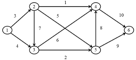
Figure 1. The network.
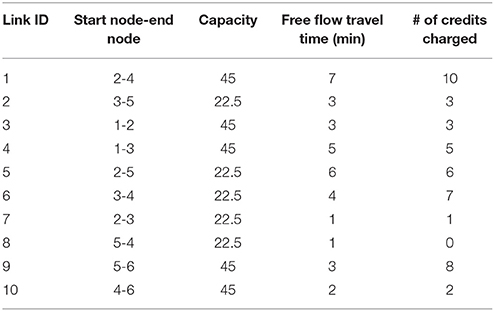
Table 1. Link parameters for the six-node network.
In this network, travelers from two user classes travel on O-D pair (1,4). Class 1 travelers have a higher VOT, 1.1 ($/min), and class 2 travelers have a lower VOT, 0.9 ($/min), which are unchanged over the planning horizon. The inverse travel demand function for user classes 1 and 2 is:
where is the potential travel demand rate, i.e., travel demand rate with zero travel cost, of travelers of class m in period t.
The planning horizon of interest is divided into 10 periods. It is assumed that the emissions coefficient ht decreases through the planning horizon due to technological advances in the automotive industry leading to lower vehicular emissions. Table 2 shows the potential travel demand rate of each user class in each period, emissions coefficient ht and issued credit rate ξt. The MPCC [(5)-(12)] and SO multi-period TCS design [(5)-(12),(64)-(66)] models are tested using the CONOPT solver (Drud, 1995) in GAMS (Rosenthal, 2015). The interest rate, st, t+1 is assumed to be constant through the planning horizon and equal to 5% unless stated otherwise for specific experiments. The issued credit rates and credit charging scheme, reported in Tables 1, 2, respectively, are used in section 6.1 to analyze the evolution of the multi-period ECP and the travel demand rates of the two user classes, and perform sensitivity analysis with respect to interest rate. Section 6.2 focuses on the optimal design of multi-period TCS to reduce the vehicular emissions.
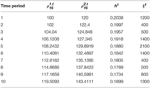
Table 2. Issued credit rates, potential travel demand, and emissions coefficients over the planning horizon.
Analysis of Multi-Period TCS
Figure 2 shows the evolution of ECPs under the multi-period TCS and multi single-period TCS. As proved in proposition 7, the multi-period TCS reduces the fluctuations in ECP compared to the multi single-period TCS. As the second and third periods have higher single-period ECPs compared to the first period, credits are transferred from the first period to the second and third periods consistent with proposition 6, which leads to the reduction of the multi-period credit prices in those periods. Travelers continue transferring credits until the multi-period ECPs in the second and third periods become equal to the sum of the multi-period ECP of the first period and the accumulated interest of the second and third periods, respectively. Hence, the multi-period ECPs of periods 1, 2 and 3 increase at the interest rate of 5%, consistent with proposition 5. Similarly, travelers transfer credits from periods 4–6 with lower single-period ECPs to periods 7–9 with higher multi-period ECPs. Figure 2 also validates proposition 7 that the multi-period TCS reduces credit price volatility compared to the multi single-period TCS irrespective of traveler heterogeneity and interest rate, highlighting its practical benefits in enabling travelers to better adapt to the TCS.
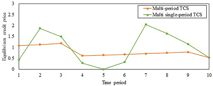
Figure 2. Equilibrium credit prices under the multi single-period TCS and multi-period TCS.
Figure 3 shows the travel demand rates for the two user classes through the planning horizon under the multi-period TCS and multi single-period TCS. The demand rates of both classes are more stable under the multi-period TCS, consistent with proposition 7, further reinforcing the benefits of implementing a multi-period TCS. Since class 2 travelers have a lower VOT and higher potential travel demand rate (as shown in Table 2), they have a higher travel demand rate compared to the travelers of class 1. Travelers store and transfer credits in periods 1, 4, 5 and 6 under the multi-period TCS; hence, the multi-period ECP is higher than the single-period ECP for those periods.
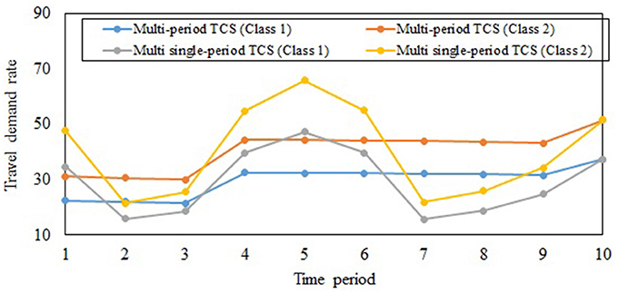
Figure 3. Travel demand rates for the two user classes under the multi-period TCS and the multi single-period TCS.
Figures 4, 5 illustrate the effects of interest rate on the evolution of multi-period ECP and the cumulative rate of stored credits over the planning horizon, respectively. As seen in Figure 4, the multi-period ECPs decrease with time if the interest rate is zero, consistent with the findings of Miralinaghi and Peeta (2016). As interest rate increases, travelers transfer fewer credits to future periods since they can gain higher monetary benefit by depositing these credits in the bank. Hence, in the context of addressing real-world goals (such as long-term reduction in emissions), it is important to factor the market effects arising from travelers' ability to earn interest by selling credits in different periods. This also highlights further the need for a multi-period TCS framework to capture both the market and traffic flow effects to address long-term planning goals. Figure 4 also illustrates that the fluctuation in multi-period ECPs increases with the interest rate. This is because travelers prefer to sell credits and earn interest rather than transfer credits as interest rate increases. Hence, as shown in Figure 5, the cumulative rate of credits that are stored over all periods reduces as interest rate increases. If the interest rate increases beyond a certain value which can be derived using proposition 8, the multi-period TCS reduces to the multi single-period TCS. As can be noted in Figure 4, the multi single-period TCS has a high level of credit price volatility consistent with proposition 7 and the insights from Figure 2.
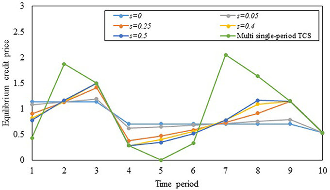
Figure 4. Impact of interest rate on the evolution of multi-period equilibrium credit price.
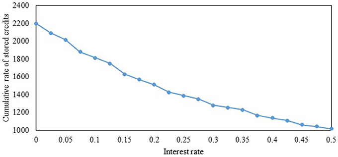
Figure 5. Impact of interest rate on the cumulative rate of stored credits over the planning horizon.
System Optimal Design of Multi-Period TCS
This section investigates the SO design of multi-period TCS to reduce vehicular emissions through the planning horizon. When the TCS is not deployed, the evolution of vehicular emissions rate and total network traffic demand rate are shown in Figures 6, 7 (which is labeled as NoTCS in these figures). Despite the increase of travel demand rates, the vehicular emissions rate decreases because of reduction of emissions coefficient through the planning horizon. To design SO multi-period TCS, the maximum ratio ϕt of travel cost for each O-D pair in period t compared to that of period t−1 is assumed to be constant through the planning horizon. The evolution of optimal vehicular emissions rate and total travel demand rate through the planning horizon under different values of ϕt are shown in Figures 6, 7 respectively. As can be seen in Figure 6, the vehicular emissions rate in each period increases as the maximum ratio of travel cost decrease. This is because the CA cannot implement a multi-TCS that increases the travel costs beyond that permitted by the maximum ratio. Under each maximum ratio ϕt, the vehicular emissions rates also decrease through the planning horizon for two reasons. First, the emissions coefficient decreases through the planning horizon. Second, as discussed earlier, the CA gradually increases credit consumption costs, leading to a decrease in the travel demand rates through the planning horizon, as shown in Figure 7. The CA can use this framework to determine the trajectory of the system-level goal (reduction in vehicular emissions) during the planning horizon, by simultaneously incorporating the objectives of reduced vehicular emissions and bounding travel costs. This enables the CA to outline the system-level emissions goals similar to the EU ETS under multi-period TCS.
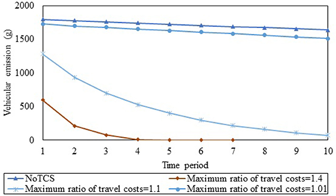
Figure 6. Evolution of vehicular emissions rate through the planning horizon under different maximum ratios of the travel cost.
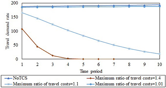
Figure 7. Evolution of travel demand rate through the planning horizon under different maximum ratios of the travel cost.
Figure 8 illustrates the cumulative value of consumed credits and cumulative expenditure of transacted credits through the planning horizon under different maximum ratios of the travel cost. The cumulative value of consumed credits is the total monetary value over the planning horizon of those credits that are paid to the CA for enabling travel. As credits are allocated freely to travelers, the cumulative expenditure of transacted credits under the TCS is the cumulative monetary amount of those credits that are purchased from other travelers in the market over the planning horizon. The cumulative value of consumed credits and cumulative expenditure of transacted credits decrease as the maximum ratio increases due to the reduction in travel demand. Further, as the maximum ratio increases, the cumulative expenditure approaches zero because travelers choose routes with credit charges identical to their credit endowments to avoid increasing credit consumption costs. As discussed in Nie and Yin (2013), any congestion pricing scheme has a TCS mirror that is equally effective in managing congestion, implying that the cumulative collected toll under that congestion pricing scheme is equal to the cumulative value of consumed credits under the TCS. As can be seen in Figure 8, the cumulative expenditure of transacted credits under the TCS is less than the cumulative value of consumed credits, which implies that travelers incur lower costs under the TCS compared to congestion pricing. Further, travelers who sell unused credits in the market are reimbursed for incurred emissions generated by other travelers. These two characteristics can increase public acceptability of TCS compared to congestion pricing. If the CA aims to generate revenue for operating roads, it can charge travelers at subsidized levels, or charge different amounts for different user classes, for receiving credit endowments instead of allocating credits for free (as assumed in this study). Then, the CA can increase the cumulative expenditure of transacted credits under multi-period TCS. The maximum cumulative expenditure of transacted credits under the TCS is equal to the revenue generated under congestion pricing. Hence, the CA can tradeoff the need to generate revenue to operate roads with the need to reduce travelers' transacted credit expenditures to increase public acceptance. In this context, the study can be extended by modifying MPCC (5)-(12) to incorporate charges for credits allocated.
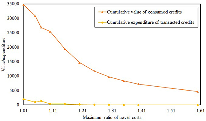
Figure 8. Cumulative value of consumed credits and cumulative expenditure of transacted credits under different maximum ratios of the travel cost.
To illustrate the importance of factoring the effects of travelers' VOT heterogeneity, we consider the case where the VOTs of classes 1 and 2 are 5 ($/min) and 1 ($/min), respectively. However, the CA designs the SO multi-period TCS assuming that all travelers are homogeneous in terms of VOT, with a value of 3 ($/min), and sets the credit price in each period to 1. Figure 9 illustrates the ECPs when the CA ignores VOT heterogeneity in the SO multi-period TCS design. The ECPs are significantly higher as illustrated by the prices being much higher than the CA-set value of 1. This reduces the ability of low-income travelers to purchase credits in the market, highlighting that issues of equity and sustainability arise when VOT heterogeneity is ignored. Figure 10 provides further insights by considering the case where the SO design factors the VOT heterogeneity correctly, labeled “Heterogeneous design” along with the incorrectly designed one assuming VOT homogeneity, labeled “Homogeneous design.” As seen in the figure, the equilibrium travel costs of class 2 (which has the lower VOT) significantly increase under the SO multi-period TCS with homogeneous design compared to the case where the VOT heterogeneity is correctly accounted for in the design. As travelers with lower incomes often have lower VOT, this scheme can be perceived as inequitable. Consequently, it will not be sustainable in practice. By contrast, when the SO design accounts for the VOT heterogeneity among travelers, the equilibrium costs reduce for class 2 travelers as the ECPs are lower when the CA correctly accounts for VOT heterogeneity.
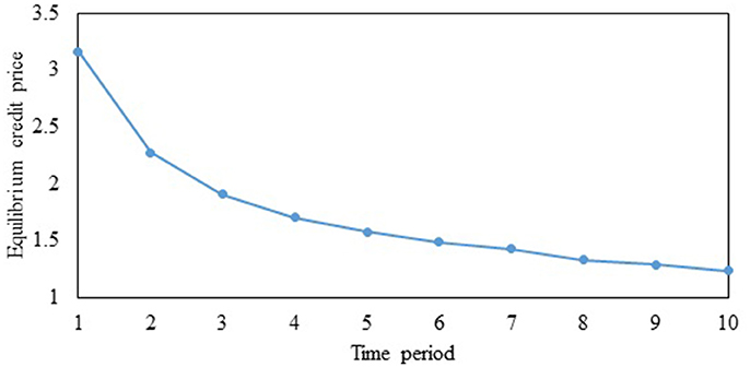
Figure 9. Equilibrium credit prices under value of time heterogeneity, but with the system optimal TCS design assuming value of time homogeneity.
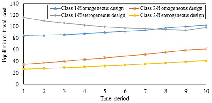
Figure 10. Equilibrium travel costs under system optimal multi-period TCS design.
To illustrate the importance of factoring interest rate for achieving long-term goals, we analyze the emissions rates over the planning horizon for two cases: (i) when interest rate is considered in SO multi-period TCS design, and (ii) when interest rate is not considered in the design. Note that as stated earlier, the interest rate is equal to 5% over the planning horizon. Figure 11 shows the vehicular emissions rates under these two cases. When the interest rate is not considered, overallocation of credits occurs under SO TCS design for periods 1–7 because the CA does not capture the higher monetary benefit of travelers resulting from selling credits and collecting interest. This ability of travelers to sell credits increases the credit supply in the market, which reduces the credit price in the market. The equilibrium credit prices under the TCS design that does not factor interest rate are shown in Figure 12. It leads to lower credit prices for periods 1–7, which leads to higher travel demands and emissions rates in those periods. After period 7, the credit allocation rates under the design that does not factor interest rate are lesser compared to the credit needs of travelers, which leads to higher credit prices in those periods. This results in higher travel demands and lower emissions rates in periods 8–10. As shown by the areas under the curves in Figure 11, the cumulative vehicular emissions over the planning horizon are correspondingly also higher. Hence, the consideration of interest rate leads to a more effective design relative to the long-term goal of reducing emissions.
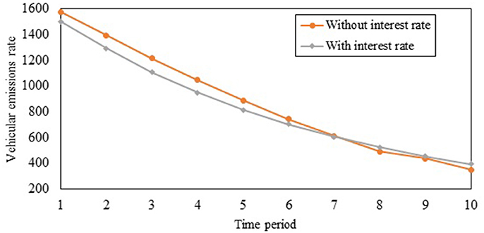
Figure 11. Vehicular emissions rates under system optimal multi-period TCS design with and without interest rate consideration.
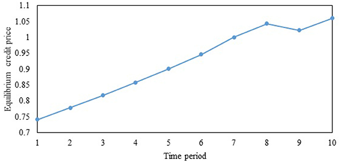
Figure 12. Equilibrium credit prices under the system optimal multi-period TCS design.
Concluding Comments
This paper investigates the SO design of multi-period TCS to minimize vehicular emissions over a planning horizon, by considering interest rate to enhance realism in the market equilibrium condition and traveler VOT heterogeneity to foster realism in the traffic equilibrium condition. In the planning context, the proposed TCS-based multi-period equilibrium modeling framework enables the CA to determine TCS parameters in advance for the planning horizon by dividing it into multiple periods. Travelers are divided into user classes based on their VOT characteristics; the average VOT of each user class is used to determine the travel cost of each route for that class. Further, since travelers can either sell unused credits or transfer them to future periods under the multi-period TCS, they can also earn interest on the monetary value of credits sold in the market, requiring the consideration of interest rate in the SO multi-period TCS design.
To design the multi-period TCS, this study first determines the equilibrium condition under VOT heterogeneity and interest rate consideration. The multi-period equilibrium condition is formulated as a VI problem, and existence and uniqueness of the equilibrium link flows, travel demand rates and ECPs are analyzed. It is shown that while multi-period ECPs can increase or decrease under positive interest rates, the credit price volatility decreases under the multi-period TCS compared to a multi single-period TCS. This enables travelers to better hedge against monetary losses arising from credit price volatility. Further, it is proved that if travelers can gain more monetary benefits by depositing the monetary value of sold credits in the bank, they do not transfer credits across periods; then, the multi-period TCS reduces to the multi single-period TCS. Using the multi-period equilibrium condition, the SO design of the multi-period TCS is proposed. It also includes a bound on the increase in travel costs in consecutive periods, which allows travelers to better adapt to credit consumption costs through the planning horizon, and consequently enhances public acceptance. Numerical experiments illustrate that the SO design of multi-period TCS enables the CA to determine the trajectory of system-level goals during the planning horizon. Further, they suggest that a multi-period TCS can entail increased public acceptance compared to congestion pricing.
The study findings suggest that the multi-period TCS should be designed by factoring interest rate and traveler VOT heterogeneity as they can significantly affect ECPs and the ability of CA to achieve system-level goals. Ignoring interest rate in the market can lead to a less-effective TCS to reduce vehicular emissions over the planning horizon. Further, even if unstable economic conditions lead to significant fluctuations in interest rates, the resulting credit price volatility can be dampened by travelers' ability to transfer credits across periods. Finally, if travelers' VOT heterogeneity is not accounted for, the TCS design can lead to socially inequitable strategies.
In this study, MPCC (5)-(12) (equilibrium condition under given multi-period TCS parameters) and MPEC [(5)-(12), (64)] (SO design of multi-period TCS) have been solved for a small network. However, there is a need to develop algorithms to solve these models for larger networks. For the SO TCS design, it has been shown that the central authority can reduce emissions rates using the multi-period TCS. This reduction depends on the maximum ratio of travel costs during the planning horizon, which can vary from 5 to 100%. Such percentage reductions are consistent with real-world targets of various agencies. For example, under the Paris agreement, the goal is to limit the worldwide temperature increase to 1.5°C. It has been shown that this reduction is equivalent to 80% by 2,033 to meet this goal (Tanaka and O'Neill, 2018). It shows that the TCS is capable of achieving this goal. Despite this capability, it is necessary to conduct further studies on the willingness of travelers to participate in this scheme and their willingness to pay, to determine the maximum ratio of travel costs during the planning horizon.
In this study, the link-based credit charging scheme is traveler-agnostic relative to emissions generated, and does not factor the traveler's vehicle type and travel mode which can significantly impact vehicular emissions. Hence, there is the need to explore TCSs that charge travelers according to their travel emissions levels. This could potentially motivate travelers to consider shifting to public transit, or vehicle types with lower emission levels. In this context, a future research direction is to investigate the design of multi-period TCS with class-specific credit charging schemes. Another research direction is to incorporate considerations such as equity in the design of a multi-period TCS. Further, there is the need to investigate the impact of the imperfect knowledge of travelers related to future interest rates. This can be captured by integrating this framework with a rolling horizon approach. Rather than solving for the entire planning horizon in the first period, the rolling horizon enables the use of near-term and medium-term forecasts with a higher degree of reliability, to derive the SO multi-period TCS design in each period for the next few periods. It can lead to more effective TCS parameters for minimizing vehicular emissions through the planning horizon. Finally, another interesting research direction is to implement the multi-period TCS over a large network with considering continuous heterogeneity of travelers in terms of VOT.
Author Contributions
All authors listed have made a substantial, direct and intellectual contribution to the work, and approved it for publication.
Conflict of Interest Statement
The authors declare that the research was conducted in the absence of any commercial or financial relationships that could be construed as a potential conflict of interest.
Acknowledgments
This work is based on funding provided by the U.S. Department of Transportation through the NEXTRANS Center, the USDOT Region 5 University Transportation Center. The authors are solely responsible for the contents of this paper.
Abbreviations
CA, Central authority; ECP, Equilibrium credit price; EU ETS, European Union emissions trading system; GHG, Greenhouse gas; MPCC, Mathematical program with complementarity constraints; MPEC, Mathematical program with equilibrium constraints; O-D, Origin-destination; SO, System optimal; TCS, Tradable credit scheme
References
Alexopoulos, A., Assimacopoulos, D., and Mitsoulis, E. (1993). Model for traffic emissions estimation. Atmos. Environ. Urban Atmos. 27, 435–446. doi: 10.1016/0957-1272(93)90020-7
Aziz, H. M. A., and Ukkusuri, S. V. (2013). Tradable emissions credits for personal travel: a market-based approach to achieve air quality standards. Int. J. Adv. Eng. Sci. Appl. Math. 5, 145–157. doi: 10.1007/s12572-013-0092-4
Bao, Y., Gao, Z., Xu, M., and Yang, H. (2014). Tradable credit scheme for mobility management considering travelers' loss aversion. Transp. Res. 68, 138–154. doi: 10.1016/j.tre.2014.05.007
Drud, A. A. (1995). A System for Large Scale Nonlinear Optimization. Tutorial for CONOPT Subroutine Library. Bagsvaerd: ARKI Consulting and Development A/S.
Ellerman, A. D., and Joskow, P. L. (2008). The European Union's Emissions Trading System in Perspective. Arlington, VA: Pew Center on Global Climate Change.
Facchinei, F., and Pang, J.-S. (2003). Finite-Dimensional Variational Inequalities and Complementarity Problems. New York, NY: Springer New York.
He, F., Yin, Y., Shirmohammadi, N., and Nie, Y. (2013). Tradable credit schemes on networks with mixed equilibrium behaviors. Transp. Res. 57, 47–65. doi: 10.1016/j.trb.2013.08.016
Johansson, O. (1997). Optimal road-pricing: Simultaneous treatment of time losses, increased fuel consumption, and emissions. Transp. Res. Transp. Environ. 2, 77–87. doi: 10.1016/S1361-9209(96)00018-1
Lawphongpanich, S., and Yin, Y. (2010). Solving the Pareto-improving toll problem via manifold suboptimization. Transp. Res. 18, 234–246. doi: 10.1016/j.trc.2009.08.006
Leggett, J. A., Elias, B., and Shedd, D. T. (2012). Aviation and the European Union's Emission Trading Scheme. Washington, DC: Congressional Research Service.
Miralinaghi, M., and Peeta, S. (2016). Multi-period equilibrium modeling planning framework for tradable credit schemes. Transp. Res. Logist. Transp. Rev. 93, 177–198. doi: 10.1016/j.tre.2016.05.013
Miralinaghi, M., Peeta, S., He, X., and Ukkusuri, S. V. (2017). Managing Morning Commute Congestion With Tradable Credit Scheme Under Commuter Heterogeneity and Loss Aversion. Washington, DC: Transportation Research Board 96th Annual Meeting. Available online at: https://trid.trb.org/view.aspx?id=1437453 (Accessed July 19, 2017).
Nagurney, A., Ramanujam, P., and Dhanda, K. K. (1998). A multimodal traffic network equilibrium model with emission pollution permits: compliance vs noncompliance. Transp. Res. Transp. Environ. 3, 349–374. doi: 10.1016/S1361-9209(98)00016-9
Nie, Y. (2012). Transaction costs and tradable mobility credits. Transp. Res. 46, 189–203. doi: 10.1016/j.trb.2011.10.002
Nie, Y., and Yin, Y. (2013). Managing rush hour travel choices with tradable credit scheme. Transp. Res. 50, 1–19. doi: 10.1016/j.trb.2013.01.004
Pigou, A. C. (1920). The Economics of Welfare, 1st Edn. London: Macmillan and Company Available online at: http://www.econlib.org/library/NPDBooks/Pigou/pgEWCover.html (Accessed June 5, 2015).
Shirmohammadi, N., Zangui, M., Yin, Y., and Nie, Y. (2013). Analysis and design of tradable credit schemes under uncertainty. Transp. Res. Rec. 2333, 27–36. doi: 10.3141/2333-04
Tanaka, K., and O'Neill, B. C. (2018). The Paris Agreement zero-emissions goal is not always consistent with the 1.5°C and 2°C temperature targets. Nat. Clim. Chang. 8, 319–324. doi: 10.1038/s41558-018-0097-x
Thuesen, G. J., and Fabrycky, W. J. (2001). Engineering Economy. Prentice Hall. Available online at: https://books.google.com/books/about/Engineering_Economy.html?id=qo1RAAAAMAAJ&pgis=1 (Accessed May 20, 2016).
Tietenberg, T. (2004). Property Rights, Economics and the Environment, ed M. D. Kaplowitz. London, UK: Routledge.
U.S. Environmental Protection Agency (2016). Inventory of U.S. Greenhouse Gas Emissions and Sinks: 1990–2014. Washington, DC. Available online at: https://www.epa.gov/sites/production/files/2016-04/documents/us-ghg-inventory-2016-main-text.pdf
Verhoef, E., Nijkamp, P., and Rietveld, P. (1997). Tradeable permits: their potential in the regulation of road transport externalities. Environ. Plan. B 24, 527–548. doi: 10.1068/b240527
Vickrey, W. S. (1969). Congestion theory and transport investment. Am. Econ. Rev. 59, 251–260. Available online at: http://www.jstor.org/stable/pdf/1823678.pdf?acceptTC=true (Accessed October 13, 2015).
Viegas, J. M. (2001). Making urban road pricing acceptable and effective: searching for quality and equity in urban mobility. Transp. Policy 8, 289–294. doi: 10.1016/S0967-070X(01)00024-5
Wallace, C. E., Courage, K. G., Hadi, M. A., and Gan, A. G. (1998). TRANSYT-7F User's Guide. Gainesville, FL: University of Florida.
Wang, X., Yang, H., Zhu, D., and Li, C. (2012). Tradable travel credits for congestion management with heterogeneous users. Transp. Res. 48, 426–437. doi: 10.1016/j.tre.2011.10.007
Xiao, F., Qian, Z. S., and Zhang, H. M. (2013). Managing bottleneck congestion with tradable credits. Transp. Res. Methodol. 56, 1–14. doi: 10.1016/j.trb.2013.06.016
Yang, H., and Huang, H.-J. (2005). Mathematical and Economic Theory of Road Pricing. Available online at: https://trid.trb.org/view.aspx?id=763678 (Accessed May 5, 2016).
Yang, H., and Wang, X. (2011). Managing network mobility with tradable credits. Transp. Res. 45, 580–594. doi: 10.1016/j.trb.2010.10.002
Yin, Y., and Lawphongpanich, S. (2006). Internalizing emission externality on road networks. Transp. Res. Transp. Environ. 11, 292–301. doi: 10.1016/j.trd.2006.05.003
Keywords: multi-period tradable credit scheme, value of time, interest rate, vehicular emissions, traffic equilibrium
Citation: Miralinaghi M and Peeta S (2018) A Multi-Period Tradable Credit Scheme Incorporating Interest Rate and Traveler Value-of-Time Heterogeneity to Manage Traffic System Emissions. Front. Built Environ. 4:33. doi: 10.3389/fbuil.2018.00033
Received: 24 March 2018; Accepted: 18 June 2018;
Published: 11 July 2018.
Edited by:
Panagiotis Ch. Anastasopoulos, University at Buffalo, United StatesReviewed by:
Grigorios Fountas, University at Buffalo, United StatesSamiul Hasan, University of Central Florida, United States
Copyright © 2018 Miralinaghi and Peeta. This is an open-access article distributed under the terms of the Creative Commons Attribution License (CC BY). The use, distribution or reproduction in other forums is permitted, provided the original author(s) and the copyright owner(s) are credited and that the original publication in this journal is cited, in accordance with accepted academic practice. No use, distribution or reproduction is permitted which does not comply with these terms.
*Correspondence: Mohammad Miralinaghi, c21pcmFsaW5AcHVyZHVlLmVkdQ==
Srinivas Peeta, cGVldGFAcHVyZHVlLmVkdQ==