Probabilistic Seismic and Tsunami Hazard Analysis Conditioned on a Megathrust Rupture of the Cascadia Subduction Zone

This paper presents a methodology for probabilistic hazard assessment for the multi-hazard seismic and tsunami phenomena [probabilistic seismic and tsunami hazard analysis (PSTHA)]. For this work, a full-rupture event along the Cascadia subduction zone is considered and the methodology is applied to a study area of Seaside, Oregon, which is located on the US Pacific Northwest coast. In this work, the annual exceedance probabilities (AEPs) of the tsunami intensity measures (IMs) are shown to be qualitatively dissimilar to the IMs of the seismic ground motion in the study area. Specifically, the spatial gradients for the tsunami IM are much stronger across the length scale of the study area owing to the physical differences of wave propagation and energy dissipation of the two mechanisms. Example results of probabilistic seismic hazard analysis and probabilistic tsunami hazard analysis are shown for three observation points in the study area of Seaside. For the seismic hazard, the joint mean annual rate of exceedance of IMs shows similar trends for the three observation points, even though for a given observation point there is a large scatter between two ground-motion IMs analyzed, which were peak ground acceleration (PGA) and spectral acceleration at a period of vibration of 0.3 s, i.e., PGA and S_a (T₁ = 0.3 s). For the tsunami hazard, the joint AEP of maximum flow depth (h_max) and maximum momentum flux ((M_F)_max) shows a high correlation between the two IMs in the study area. The joint AEP at each of the three observation points follows a particular Froude number (Fr) due to the local site-specific conditions rather than the distributions of fault slip distributions used to generate the scenarios that are the basis of the AEP maps developed. The joint probability distribution of h_max and (M_F)_max throughout the study region falls between 0.1 ≤ Fr < 1.0 (i.e., the flow is subcritical), regardless of return interval (500-, 1,000-, and 2,500-year). However, the peak of the joint probability distribution with respect to h_max and (M_F)_max varies with the return interval, and the largest values of h_max and (M_F)_max were observed with the highest return intervals (2,500 years) as would be expected. The results of the PSTHA can be the basis for a probabilistic multi-hazard damage and loss assessment and help to evaluate the uncertainties of the multi-hazard assessments.

Introduction

Over the past decade and a half, megathrust earthquakes accompanied by near-field tsunamis have devastated coastal regions throughout the world, including the 2004 Indian Ocean tsunami (e.g., Jaffe et al., 2006; Rossetto et al., 2007), events in Chile in 2010 (e.g., Mas et al., 2012), and the 2011 Tohoku tsunami (e.g., Mori et al., 2013). These events remind us that when assessing for life safety, it is often desirable to plan for a “worst case” or “most credible” scenario. However, when considering damage to the built environment, it is often more practical to employ risk-informed decision-making to help minimize the overall damage, annualized financial loss, and increase the rate of recovery. In other words, risk-based decisions can increase the overall resilience of a community to earthquake and tsunami events. However, risk-based methods require a probabilistic understanding of the hazard. The case of subduction zone (SZ) earthquakes and tsunamis is particularly challenging because of the multi-hazard phenomena. A large building located in the megathrust earthquake region and in a potentially tsunami prone zone, for example, will first experience intense ground shaking followed by the subsequent hydrodynamic demands imposed by the tsunami. Liquefaction, local scour, landslides, debris, and other cascading consequences further exacerbate the problem. This paper marks one of the first attempts to provide a methodology for conducting a joint hazard analysis, which is termed as probabilistic seismic and tsunami hazard analysis (PSTHA), by combining probabilistic seismic hazard analysis (PSHA) with probabilistic tsunami hazard analysis (PTHA) based on a consistent process for concurrent earthquake occurrence and tsunami generation. As an illustrative example, the PSTHA is applied to a coastal community based on a conditional rupture of the Cascadia subduction zone (CSZ) along the northwest coast of North America.

Background and Literature Review

Probabilistic seismic hazard analysis provides the evaluation of annual frequencies of exceedance of ground motion intensity measures (IMs) [typically designated by peak ground acceleration (PGA) or by linear elastic damped response spectral ordinates at specific periods of vibration] at a site. The result of a PSHA is a seismic hazard curve [annual frequency of exceedance versus ground-motion intensity measure (IM) amplitude], a uniform hazard spectrum (spectral amplitude versus structural period, for a fixed annual frequency of exceedance), or conditional mean spectrum (Baker, 2011; Lin et al., 2013). First reports of PSHA date back to the 1960s. Since then, PSHA has become the basis for seismic assessment and design of new and existing engineered facilities ranging from civil structures, such as buildings and bridges, to critical facilities, such as nuclear power plants. In PSHA, all possible earthquake fault sources contributing to the hazard need to be characterized first. Second, ground-motion prediction equations (GMPEs) are used to relate ground-motion IMs to variables describing earthquake source, path, and site effects. Extensive research has been performed on GMPEs for use in PSHA. Douglas (2003, 2011, 2016) summarized over 400 GMPEs that were developed since 1964–2016 for estimation of PGA and over 250 GMPEs for estimation of spectral ordinates at a site. Douglas and Edwards (2016) provides a recent discussion of current and future trends in ground-motion prediction. Stewart et al. (2015) provides a discussion of the selection of GMPEs for hazard assessments for the three principal tectonic regimes: active crustal regions, SZs, and stable continental regions for a global earthquake model. Of interest to this paper, Stewart et al. (2015) recommended the use of three models for SZ ground-motion predictions, “BC Hydro” model of Abrahamson et al. (2016), the global earthquake model described in Atkinson and Boore (2003), and the model in the study by Zhao et al. (2006). The BC Hydro model was developed using different data sets of SZ strong-motion recordings (e.g., Crouse et al., 1988; Crouse, 1991; Youngs et al., 1997; Atkinson and Boore, 2003, 2008; Zhao et al., 2006; Lin and Lee, 2008). While GMPEs are most often used for PSHA, it is worth noting that other methods for generating the IMs that involve the generation of synthetic ground motions have also been recently proposed, however, all involving extremely computational intensive methods. These methods that could serve as alternatives to the GMPEs include kinematic earthquake models (e.g., Olsen et al., 2008; Frankel et al., 2014; Pulido et al., 2015; Iwaki et al., 2016), stochastic finite-fault ground-motion methods (e.g., Atkinson et al., 2009), or hybrid broadband ground-motion methods (e.g., Atkinson et al., 2011; Skarlatoudis et al., 2015).

Relative to PSHA, only recently has there been much work on PTHA. Mori et al. (submitted)¹ summarized 30 PTHA studies conducted worldwide, all but one of which were conducted after the 2004 Indian Ocean tsunami. Prior to the 2004 event, tsunami hazards were generally characterized by “worst credible” or “worst case” scenarios. Rikitake and Aida (1988) were the first to use historical records of past run-up events to characterize the probability of the tsunami run-up hazard in Japan. Subsequent to the 2004 event and with the more recent SZ tsunami events in Chile in 2010 and in Japan in 2011, there has been an increasing interest in developing PTHA. Studies have focused on regions throughout the Pacific Rim, including Japan (Burroughs and Tebbens, 2005; Annaka et al., 2007; Yanagisawa et al., 2007; Fukutani et al., 2015; and Goda and Song, 2016), the US Pacific Coast and Canada (Geist and Parsons, 2006; González et al., 2009; Thio and Somerville, 2009; Priest et al., 2010; Witter et al., 2013; Leonard et al., 2014; and Park and Cox, 2016), South China Sea (Liu et al., 2007; Li et al., 2016), New Zealand, and Australia (Power et al., 2007, 2013; Burbidge et al., 2008; and Mueller et al., 2015), as well as places in Europe (Tinti et al., 2005; Grezio et al., 2010; Anita et al., 2012) and the Northwestern Indian Ocean (Thio et al., 2007; Heidarzadeh and Kijko, 2011). As explained in the study by see text footnote 1, the PTHA generally uses one of three approaches for the tsunami generation: (1) historical record approach, (2) logic-tree approach, and (3) random phase approach. Generally, the historical record of tsunamis is not sufficient to build a credible probabilistic model. Therefore, the second two approaches are favored. The logic-tree approach (e.g., Park and Cox, 2016) is based on combinations of slip conditions (e.g., magnitude, peak slip location, and slip distribution), and these combinations are given a weighting based on expert opinion, historical record, or equal weighting in some cases. For the random phase approach (e.g., Goda et al., 2014), the slip distributions are created by an assumed slip wavenumber spectrum using random phases. For this paper, the logic-tree approach is used since it is straightforward to combine PTHA with the PSHA. In general, the output of the PTHA focuses on the flow depth at the shoreline, the maximum extent of inundation for planning, the evaluation of annual exceedance probabilities (AEPs), or the estimation of the extent of damage through a probabilistic tsunami damage analysis (e.g., Wiebe and Cox, 2014; Park et al., 2017).

The authors are aware of only one study by De Risi and Goda, 2016 (DG16 hereafter), which considers the combined PSTHA. In that paper, the authors present a consistent method to account for a common rupture process. They use GMPEs based on magnitude and rupture distance to quantify the shaking intensity at a particular location subjected to a SZ earthquake, and then solve the shallow water wave equations for tsunami propagation and inundation from the source to the site of interest. The main output of their work is seismic hazard curves and tsunami hazard curves that represents the mean annual rate (MAR) of exceedance of a given IM. Their generalized framework was applied for assessing combined earthquake and tsunami hazard at a single location on the coast line of Sendai City based on the subduction fault plane in the Tohoku region of Japan.

Study Objectives and Outline

Similar to the work of DG16, the objective of this work is to develop a consistent framework for a multi-hazard analysis considering large magnitude SZ earthquakes and a subsequent near-field tsunami. However, the study performed herein is developed for a different site with a different methodology to define earthquake and tsunami sources when compared to DG16. The long-term objective is to be able to use the PSTHA as the basis for a probabilistic multi-hazard damage assessment to quantify the separate contributions of seismicity and tsunami hazards in the estimation of damage to the built environment at a community scale or for design of specific infrastructure elements such as a critical facility. A general methodology is first presented in Section “Methodology,” with a general review of the combined probabilistic hazard analysis (PHA) methodology proposed (see General PHA Methodology), the earthquake fault source models and their characteristics (see Earthquake Fault Source Models and Their Characteristics), the GMPEs used (see Earthquake Simulation), and the tsunami generation, propagation, and inundation (see Tsunami Generation, Propagation, and Inundation). Then, the multi-hazard logic-tree model is presented (see Multi-Hazard Logic-Tree Model), and the methods to estimate the AEP (see Estimates of the AEP) are presented next. In Section “Application: Full-Rapture Event of the CSZ Impacting the City of Seaside, OR,” the methodology is applied to an application example in which the combined seismic and tsunami hazard are quantified for the City of Seaside on the Oregon Coast of the US Pacific Northwest, conditional on a full rupture of the CSZ. In this application, the CSZ earthquake source model, and the geological, geographic, and morphological features of the City of Seaside, Oregon, are characterized first (see Characterization of the Source) and then details of the CSZ fault model and tsunami model (see CSZ Fault Modeling) are provided. In Section “Results,” results are presented in terms of the seismicity (see Seismicity) and tsunami intensity (see Tsunami Intensity) estimated for the area of interest. A spatial representation of both the seismic and tsunami intensity is presented, including the study of the granularity needed to characterize the hazards and joint distribution for different vector-valued IMs (see Spatial Representations Seismic and Tsunami Hazard). Finally, in Section “Summary, Conclusion, and Future Work,” discussion and summary of the results are provided, followed by the conclusion and recommendations for future research.

Methodology

The methodology for consistent PSTHA is presented in this section. The methodology behind PSHA is well known (e.g., McGuire, 2004). However, a few adaptations are required for performing the combined PSTHA. The statistical earthquake model behind PSTHA is the same for PSHA and PTHA, although in PSHA the earthquakes generated solely inland do not contribute to the tsunami hazard. Even though the statistical earthquake model may be the same, the methods used in PSHA and PTHA for propagation of the effects of a fault slip to a specific site of interest vary. For PSHA, GMPEs are most often used. The GMPEs relate a certain moment release on an earthquake source (a line source or an area source) and the source-to-site rupture distance (or in a few instances, the hypocentral distance) to the ground-motion IMs. For the tsunami hazards, and due to the way tsunamis are generated, instead of using equations analogous to GMPEs, the conscientious decision is made herein of using the waveform excitation and propagation approach by solving non-linear shallow water equations [e.g., the “Method of Splitting Tsunami” (MOST) model, Titov et al., 2011] in which an earthquake, transoceanic propagation, and inundation of dry land are modeled. This type of detailed modeling of the tsunami propagation is analogous to computationally intensive recent trends in PSHA, which involves the use of methods for generating ensembles of synthetic ground-motion time histories as described above.

General PHA Methodology

The general formulation presented here is aimed at developing the probabilistic earthquake and tsunami hazard at a site. In this formulation, the first topic that has to be addressed is the definition of an IM for the hazard. For example, with respect to earthquake ground shaking, typical measures of interest are spectral acceleration (S_a), while common IMs used for the tsunami hazard are the inundation flow depth (h), flow velocity (V), and specific momentum flux (M_F = hV²). Since there is great uncertainty in the quantification of the earthquake that induces ground shaking and possible tsunamis, be it in the focal mechanism including definition of the location (e.g., location of the epicenter, extension of fault rupture), size (magnitude), and resulting intensity of a future earthquake at a specific site of interest, PSHA (e.g., Cornell, 1968; McGuire, 1995; Kramer, 1996) was developed as an analytical tool to characterize the seismic hazard probabilistically. PSHA has become the most widely used method for assessing seismic hazard at a specific site. More recently, PTHA has also been developed (PTHA—e.g., Geist and Parsons, 2006; Annaka et al., 2007; Power et al., 2007) as reviewed by see text footnote 1 and summarized in Section “Background and Literature Review.”

The general PHA provides the MAR(λ) of IM exceeding an intensity measure value im that is computed using the Total Probability Theorem (Benjamin and Cornell, 1970), by integrating the contributions of all possible tsunami-seismogenic sources, and for each of the sources, all possible values of earthquake magnitude as

${\mathrm{\lambda }}_{\mathit{IM}>\mathit{im}}\left(\mathit{im}\right)={\displaystyle \sum _{i=1}^{N_{\text{sources}}}}{\mathrm{\lambda }}_i\left(M\ge m_{\min }\right)\times {\int }_{\mathrm{\Theta }}{\int }_{m_{\min }}^{m_{\max }}P\left(\left.\mathit{IM}>\mathit{im}\right|\mathrm{\Theta },M\right)s_{{\mathrm{\Theta }}_i}\left(\left.\mathrm{\Theta }\right|M\right)f_{M_i}\left(m\right)\mathit{dm}d\mathrm{\Theta }$ (1)

where N_sources denotes the total number of seismic sources contributing to the hazard at the site, λ_i(M ≥ m_min) is the MAR of occurrence of earthquakes with magnitude greater than a lower bound threshold value, m_min, of seismic source i, P (IM > im|Θ,M) represents the probability that intensity measure IM will exceed a given intensity value im at the site conditional on a given magnitude M and source parameters Θ, $s_{{\mathrm{\Theta }}_i}\left(\left.\mathrm{\Theta }\right|M\right)$ represents the characteristic probability density function (PDF) of earthquake source parameters Θ obtained from a hazard parameter prediction model conditional on the magnitude of the earthquake, and the function $f_{M_i}\left(m\right)$ denotes the PDF of the magnitude M given the occurrence of an earthquake on seismic source i.

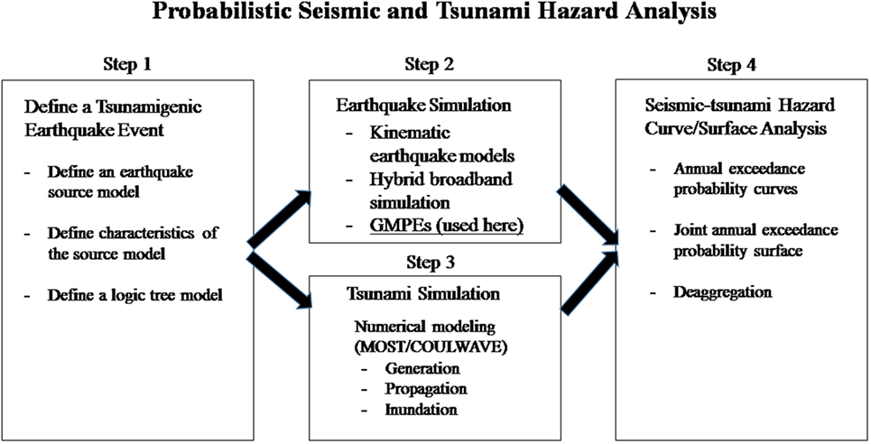
In Eq. 1, it is assumed that earthquake occurrences at different seismic sources are statistically independent (in terms of occurrence time, scaling relationship, M, etc.), implying that earthquake occurrences from all possible sources can be assumed to follow a Poisson process. It is also assumed that within each seismic source i, the magnitude M_i earthquake events are statistically independent. Thus, the summation in Eq. 1 considers the contributions from all seismic sources while the integrations over M_i and source parameters account for earthquakes of all possible magnitudes and source parameters conditional on the magnitude for each seismic source, respectively. In Eq. 1, the conditional probability P(IM > im|Θ,M), with im > 0, represents the complementary cumulative distribution function (CCDF) of the IM conditional on M and Θ. Figure 1 illustrates the steps that can be used to compute the probabilistic seismic and tsunami hazard relationships. In Step 1, the earthquake fault source models and characteristics of the earthquake source models are defined. In Step 2, the ground-motion IMs at a given site are obtained through the earthquake simulation, performed through either explicit source-to-site wave propagation models and synthetic ground-motion generation or, most commonly, with GMPEs. In Step 3, the tsunami is simulated, including tsunami generation, propagation and inundation modeling. In Step 4, the seismic-tsunami hazard curves and surfaces are determined. It is notable that Step 2 (seismic simulations) and Step 3 (tsunami simulations) are produced from a consistent earthquake event.

FIGURE 1

Figure 1. Flow chart of methodology used for probabilistic seismic and tsunami hazard analysis.

Earthquake Fault Source Models and Their Characteristics

To describe the distribution of earthquake magnitudes in a given region of interest, the Gutenberg–Richter relationship (GR) is widely adopted. The GR relationship is given by

$\log {\mathrm{\lambda }}_m=a-\mathit{bm}$ (2)

where λ_m is the MAR of exceedance of an earthquake of magnitude m, a represents the overall rate of earthquakes in a region of interest, and b represents the relative ratio of small and large magnitudes. The parameters a and b are estimated based on statistical analysis of the database of seismicity for the seismic source zone of interest. The GR relationship is developed from a regional dataset of seismicity accounting for many different source zones and has been found to be inadequate to represent the earthquake recurrence relationship for the tail-end of the magnitude–frequency distribution representing large magnitude earthquakes (Schwartz and Coppersmith, 1984; Wesnousky, 1994). Several models have been proposed to address the shortcomings of the GR recurrence law (Kagan, 1997, 2002a; Bird and Kagan, 2004). For SZs, such as the CSZ used as an example in this paper, a Tapered Gutenberg–Richter (TGR) distribution has been shown to be a robust model (Rong et al., 2014). The TGR is expressed as a function of the seismic moment M₀, instead of magnitude m and an exponential taper is applied to the number of events with very large seismic moment. The TGR CCDF is given by Kagan (2002a)

$F\left(M_0\right)={\left(\frac{{M_0}_t}{M_0}\right)}^{\mathrm{\beta }}\exp \left(\frac{M_{0^t}-M_0}{M_{0c}}\right),\text{ for }{M_0}_t\le M_0<\infty$ (3)

where β is the index parameter of the distribution, and β = (2/3)b, M_0c is the corner moment, and M_0t is the threshold moment above which the earthquake catalog is assumed to be complete. The conversion between seismic moment M₀ and moment magnitude m is given by

$M_0={10}^{1.5m+C}$ (4)

where C = 9 − 9.1. The corner moment M_0c can be estimated using the seismic moment conversion principle (Kagan, 2002b) and given approximately by

${M_0}_c={\left[\frac{\mathrm{\chi }{\dot{M}}_T\left(1-\mathrm{\beta }\right)}{{\mathrm{\alpha }}_t{M}_{0t}^{\mathrm{\beta }}\mathrm{\Gamma }\left(2-\mathrm{\beta }\right)}\right]}^{1/\left(1-\mathrm{\beta }\right)}$ (5)

where χ is the seismic coupling coefficient, ${\dot{M}}_T$ is the tectonic moment rate, α_t is the recurrence rate for earthquake with moment M_0t and greater, and Γ is the gamma function. Equation 5 can be used to derive the recurrence interval as

$T\left(M_{\text{0}t}\right)=\left[\frac{1}{1-\mathrm{\beta }}\right]\frac{M_{\text{0}t}^{\mathrm{\beta }}{M}_{\text{0}c}^{1-\mathrm{\beta }}}{{\dot{M}}_T}\mathrm{\Gamma }\left(2-\mathrm{\beta }\right)\text{exp}\left(\frac{M_{\text{0}t}}{M_{\text{0}c}}\right)$ (6)

The TGR CCDF can be rewritten in terms of magnitude m and given as

$F\left(m\right)={\left[{10}^{1.5\left(m_t-m\right)}\right]}^{\mathrm{\beta }}\exp \left[{10}^{1.5\left(m_t-m_c\right)}-{10}^{1.5\left(m-m_c\right)}\right]$ (7)

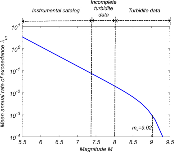
Rong et al. (2014) estimated the probable maximum earthquake that is likely to occur within a given time for circum-Pacific SZs using TGR distributions. For the CSZ, using maximum likelihood estimation method, the values of β = 0.59 and m_c = 9.02 were estimated considering the 10,000-year paleoseismic record based on the turbidite studies by Goldfinger et al. (2012), coupled with the limited number of instrumental earthquake data. In the implementation performed, it is convenient to convert the continuous distribution of magnitudes into a discrete set of possible magnitudes m_j, which are given by

$P\left[M=m_j\right]=G\left(m_j+0.\mathrm{5\Delta }m\right)-G\left(m_j-0.\mathrm{5\Delta }m\right)$ (8)

where the G(m) = 1 − F(m) is the cumulative density function and Δm is the adopted discretization interval.

Figure 2 shows the median earthquake recurrence relationship developed for the CSZ using a TGR distribution (Eqs 3–7) and with β = 0.59 and m_c = 9.02, as recommended by Rong et al. (2014) for the CSZ. According to the TGR distribution shown in Figure 2, m ≥ 8.8 earthquakes are expected with a return period of 500 years (λ_m = 0.002), while m ≥ 9.0 earthquakes are expected with a return period of 1,000 years (λ_m = 0.001). Goldfinger et al. (2012) reconstructed the large earthquake history of the CSZ for approximately10,000 years based on strong shaking-induced turbidite deposits in marine sediments and onshore paleoseismic records. The study suggested four types of earthquake rupture along the CSZ based on the interpretation of the turbidite data during the past 10,000 years: (1) 19–20 full-margin or nearly full-margin ruptures, (2) 3–4 ruptures along the 50–70% of the southern margins, (3) 10–12 southern ruptures from central Oregon southward, and (4) 7–8 southern Oregon/northern California ruptures. Though the turbidite data do not provide direct indication of the probable earthquake magnitudes, Goldfinger et al. (2012) estimated the earthquake magnitudes of different rupture events based on the relations observed among the rupture length (distance between offshore core sites containing turbidites from same events), turbidite thickness, and turbidite mass and estimated that full-rupture events constituted m = 8.7~9.3. Considering 20 full rupture over the past 10,000 years, the MAR of full-rupture events ${\mathrm{\lambda }}_{\mathit{full}-\mathit{rupture}}\approx \frac{20}{10,000}=0.002$, which is consistent with the λ_m≥8.8 = 0.002 estimated by Rong et al. (2014) using TGR distribution shown in Figure 2.

FIGURE 2

Figure 2. Tapered Gutenberg–Richter relationship for Cascadia subduction zone.

Earthquake Simulation

Near-field ground motions are strongly affected by the heterogeneity of earthquake rupture processes, such as slip distribution, rupture directivity, and the acceleration and deceleration of the rupture front. To estimate the ground motion quantitatively for a seismic hazard assessment, characterization of this heterogeneity is essential, and usually accounted for in ground-motion hybrid broadband simulation procedures (e.g., Somerville et al., 2012) or 3D simulations of earthquake event scenarios (e.g., Olsen et al., 2008; Delorey et al., 2014). While these explicit source-to-site wave propagation models and synthetic ground-motion generation models are extremely useful, especially in generating synthetic waveforms, these typically involve very large number of computations in large parallel computing centers, which is currently still not feasible when performing probabilistic seismic hazard analyses. Instead, when performing PSHA, GMPEs are still typically used today.

In this study, GMPEs, which are dependent on the local and regional site conditions, are used to simulate the ground-motion IMs. The recently developed Abrahamson et al. (2016) GMPE, which is based on the global datasets on SZ earthquakes described in Section “Background and Literature Review” is used. The functional form of this GMPE for interface SZ earthquakes is given by:

$\begin{array}{l}\ln \left({\mathit{Sa}}_{\text{interface}}\right)={\mathrm{\theta }}_1+{\mathrm{\theta }}_4\mathrm{\Delta }{C}_1+\left({\mathrm{\theta }}_2+{\mathrm{\theta }}_3\left(M-7.8\right)\right)\text{ ln}\left(R_{\text{rup}}+C_4\exp \left({\mathrm{\theta }}_9\left(M-6\right)\right)\right)\hfill \\ +{\mathrm{\theta }}_6{R}_{\text{rup}}+f_{\text{MAG}}\left(M\right)+f_{\text{FABA}}\left(R_{\text{rup}}\right)+f_{\text{site}}\left(\text{PG}{\text{A}}_{1,000},V{s}_{30}\right)+\mathrm{\sigma ϵ}\hfill \end{array}$ (9)

where θ_i are regression parameters, R_rup is the closest distance to the rupture area from site, Vs₃₀ is the shear wave velocity of the uppermost 30 m of soil, PGA_1,000 is the median PGA corresponding to Vs₃₀ = 1,000 m/s, σ is the total SD, which is obtained combining intra-event uncertainty ϕ and inter-event uncertainty τ, and ϵ is the standard normal error term. In this study, only the intra-event uncertainty ϕ is considered since only the CSZ is used for hazard analysis. The magnitude scaling term is given by

$f_{\text{MAG}}\left(M\right)=\left\{\begin{array}{c}{\mathrm{\theta }}_4\left(M-\left(C_1+\mathrm{\Delta }{C}_1\right)\right)+{\mathrm{\theta }}_{13}{\left(10-M\right)}^2,\text{for }M\le C_1+\mathrm{\Delta }{C}_1\hfill \\ {\mathrm{\theta }}_5\left(M-\left(C_1+\mathrm{\Delta }{C}_1\right)\right)+{\mathrm{\theta }}_{13}{\left(10-M\right)}^2,\text{for }M>C_1+\mathrm{\Delta }{C}_1\hfill \end{array}\right.$ (10)

where C₁ = 7.8, and the ΔC₁ term represents the epistemic uncertainty around the distinct break in magnitude scaling between frequent smaller magnitudes events and rare large interface events. The forearc and backarc scaling term in Eq. 9 is given by

$\begin{array}{l}{f}_{\text{FABA}}\left(M\right)=\left[{\mathrm{\theta }}_{15}+{\mathrm{\theta }}_{16}\ln \left(\frac{\text{max}\left(R_{\text{rup}},100\right)}{40}\right)\right]F_{\text{FABA}};\hfill \\ F_{\text{FABA}}=\left\{\begin{array}{cc}0,\hfill & \text{for forearc or unknow sites;}\hfill \\ 1,\hfill & \text{for backarc sites}.\hfill \end{array}\right.\hfill \end{array}$ (11)

The model for site response scaling is given by

$\begin{array}{c}{f}_{\text{site}}\left({\text{PGA}}_{1,000},V{s}_{30}\right)=\left\{\begin{array}{cc}\left[{\mathrm{\theta }}_{12}\ln \left(\frac{V_S^{\ast }}{V_{\text{lin}}}\right)\right]-b\ln \left({\text{PGA}}_{1,000}+c\right)+b\mathrm{\hspace{0.17em}ln}\left({\text{PGA}}_{1,000}+c{\left(\frac{V_S^{\ast }}{V_{\text{lin}}}\right)}^n\right),\hfill & \text{for }{V}_{s30}<V_{\text{lin}}\hfill \\ \left[{\mathrm{\theta }}_{12}\mathrm{\hspace{0.17em}ln}\left(\frac{V_S^{\ast }}{V_{\text{lin}}}\right)\right]+b\mathrm{\hspace{0.17em}ln}\left(\frac{V_S^{\ast }}{V_{\text{lin}}}\right),\hfill & \hfill \text{for }{V}_{s30}\ge V_{\text{lin}}\end{array}\right.\hfill \\ V_S^{\ast }=\left\{\begin{array}{cc}1,000,\hfill & \text{for }{V}_{s30}>1,000;\hfill \\ V_{s30},\hfill & \text{for }{V}_{s30}\le 1,000.\hfill \end{array}\right.\hfill \end{array}$ (12)

All other model coefficients in Eqs 9–12 are listed in the study by Abrahamson et al. (2016).

Tsunami Generation, Propagation, and Inundation

In general terms, the tsunami hazard at a particular site requires the three steps of (1) tsunami generation, (2) propagation, and (3) inundation. For most modeling efforts, tsunami generation is given as an initial surface water displacement along the fault. The Okada (1985) model, which is based on the linear co-seismic dislocation of fault slips, is often used for simplicity, and the initial displacement is assumed to occur simultaneously along the fault.

Tsunami propagation is generally considered a solved problem in that the equations are well defined for long wave propagation in the open ocean. Of course, the propagation phase requires accurate knowledge of the underlying bathymetry which affects the wave through refraction, diffraction, and shoaling. The third phase, tsunami inundation, considers the flow of water over dry land. This is considered a difficult problem to solve because of the complex interaction of the flow with the built and natural environment that is also changing due to the destructive nature of the flow. However, most inundation models assume “bare earth” conditions, that is a digital elevation model (DEM) in which the natural and built environments are removed. Typically, the effects of the vegetation and structures are replaced by a suitable friction factor, although there are additional uncertainties in this step (e.g., Park et al., 2013; Bricker et al., 2015).

In this study, the logic-tree model by Park and Cox (2016) is applied for tsunami generation to characterize the fault slip. The slip model from the study by Park and Cox (2016) characterizes the randomness of fault slip distribution at the CSZ as a Gaussian shape, parameterized in terms of the moment magnitude, peak slip location, and a fault slip shape as

$f\left(Y\prime /\mathit{dL}|\mathrm{\alpha },\mathrm{\beta }\right)=\frac{1}{\mathrm{\beta }\sqrt{\mathrm{2\pi }}}\exp \left(\frac{-{\left(Y\prime /\mathit{dL}-\mathrm{\alpha }\right)}^2}{{\mathrm{2\beta }}^2}\right)$ (13)

where α and β are the slip distribution parameters along a rupture strike direction (Y ′), and dL is the unit length of sub-fault utilized in the slip model. Each parameter α and β controls the location of the peak slip and the shape of slips. A total of 72 scenarios from the three seismic moments, three slip shapes, and eight peak slip locations are proposed for the full-length rupture CSZ event. The occurrence rate of each seismic moment estimated from the paleoseismic data at CSZ (Goldfinger et al., 2012). Each of the fault slip distributions are determined from the slip model and applied to the ComMIT/MOST model (Titov et al., 2011) as an input to simulate the tsunami generation and propagation parts. Although MOST can also be used for the inundation phase, the software COULWAVE (Lynett et al., 2002) is used to model this final step (Park and Cox, 2016).

Multi-Hazard Logic-Tree Model

The generic multi-hazard logic tree is presented in Figure 3. The first step is to identify all tsunamigenic earthquakes that could potentially affect the site of interest. These earthquakes are then classified as near-field or far-field earthquakes depending on the source location with respect to the site. For each of the potential fault sources, the next step is to use an appropriate recurrence model. As mentioned in Section “Earthquake Fault Source Models and Their Characteristics,” the widely used modified-GR underpredicts the recurrence rate for large magnitude tsunamigenic earthquakes and hence TGR (Kagan, 2002a) and other characteristic moment–frequency distributions (e.g., Wesnousky, 1994) are preferred. Since most of the GMPEs use a distance metric of closest distance from the site to the rupture plane (R_rup), the depth of rupture which determines the position of the rupture edge close to the site of interest can have significant effect on the ground-motion intensity observed. Several geophysical models are available to determine the rupture depth and can be used for a specific fault of interest. As for example, for 2014 National Seismic Hazard Map of United States, three geophysical models were used to constrain the eastern edge of the CSZ rupture zone (Frankel et al., 2015).

FIGURE 3

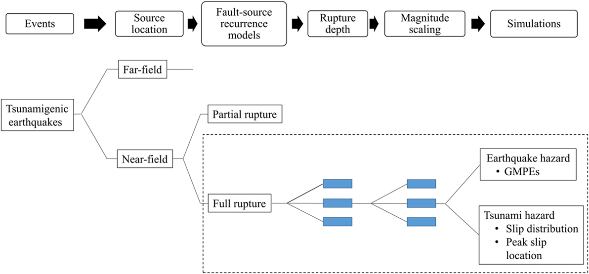
Figure 3. Generic logic tree for the probabilistic seismic and tsunami hazard analysis. The dashed box shows the full-rupture event considered in the example applied to the Cascadia subduction zone.

Reliable magnitude scaling relationships for subduction earthquakes is a prerequisite for accurate estimation of earthquake and tsunami hazard intensities. There are several magnitude scaling relationships available in the literature that are derived from global observation of earthquakes on the plate interface of SZ (Papazachos et al., 2004; Strasser et al., 2010; Murotani et al., 2013; Goda et al., 2016; Skarlatoudis et al., 2016). Of these, Skarlatoudis et al. (2016) compiled an updated database of interface earthquakes that occurred worldwide in last decade in the major SZs (e.g., 2004 M 9.1 Sumatra, 2010 M 8.8 Chile, 2011M 9.0 Japan earthquake) and proposed new and improved source scaling laws with reduced uncertainty compared to other currently available source scaling laws for subduction earthquakes. Once the appropriate source magnitude and scaling laws are identified, the final step is to perform the earthquake and tsunami simulations for a multiple logic-tree branch. In the case of earthquakes, GMPEs are utilized, which typically make use of the M and R_rup as the input parameter to compute the ground-motion IMs at the site. On the other hand, for tsunamis, the details of the slip distribution (e.g., slip shape, peak slip location within rupture zones) and seismic moment for a given rupture are critical input parameters needed to compute the tsunami hazard intensity at a given site.

Estimates of the AEP

Four IMs were selected for the PSTHA, including the PGA, the 5% damped linear elastic spectral acceleration at a fundamental period of vibration of 0.3 s [S_a(T₁) = 0.3 s], the maximum flow depth (h_max), and the specific maximum momentum flux (M_F)_max because these IMs are often linked with structural damage at a structure scale (e.g., Faggella et al., 2013; Gidaris et al., 2016). Here, the flow depth is the net elevation of the free surface elevation above the local land elevation, and the specific momentum flux is given by the product of the flow depth with the square of the flow velocity (M_F = hV²).

The Poisson process (Cornell, 1968) is used to estimate the AEP of both earthquake and tsunami hazard curves at a specific location. The probability of IMs exceeding a certain level of that hazard conditional on a given time t is equal to the probability of at least one event occurring in time t, and is given by

$P\left[\mathit{IM}>\mathit{im}|t\right]=1-e^{-\mathrm{\lambda }t}$ (14)

where λ is the mean occurrence rate at which the IM will exceed a specific im at a given location during the time t. The MAR exceedance of each IM is computed using Eq. 1.

The AEP surfaces for the joint seismic-tsunami hazard can be computed using the formulation presented next, designated here as vector-valued probabilistic seismic and tsunami hazard analysis (VPSTHA). The presentation starts from the definition of the joint mean rate density (MRD) of the hazard (e.g., Bazzurro, 1998; Barbosa, 2011), here expanded to account for IMs related to ground-motion shaking intensity as well as tsunami IMs. For a vector of ground-motion and/or tsunami intensity parameters IM = {IM₁,IM₂}, the joint MRD of the hazard is given by

${\text{MRD}}_{{\mathit{IM}}_1,{\mathit{IM}}_2}\left({\mathit{im}}_1,{\mathit{im}}_2\right)={\displaystyle \sum _{i=1}^{N_{\text{sources}}}}{\mathrm{\lambda }}_i\left(M\ge m_{\min }\right)\times {\int }_{\mathrm{\Theta }}{\int }_M{f}_{{\mathit{IM}}_1,{\mathit{IM}}_2}\left(\left.{\mathit{im}}_1,{\mathit{im}}_2\right|\mathrm{\Theta },M\right)s_{{\mathrm{\Theta }}_i}\left(\left.\mathrm{\Theta }\right|M\right)f_{M_i}\left(m\right)\mathit{dm}d\mathrm{\Theta }$ (15)

where $f_{{\mathit{IM}}_1,{\mathit{IM}}_2}\left(\left.{\mathit{im}}_1,{\mathit{im}}_2\right|\mathrm{\Theta },M\right)$ is the joint PDF of IM₁ and IM₂ conditional on earthquake of magnitude M and source parameters Θ. Once the MRD is defined, the MAR of events at the site with IM₁ and IM₂ being between im_1,1 < IM₁ ≤ im_1,2 and im_2,1 < IM₂ ≤ im_2,2, respectively, is given by:

${\mathrm{\lambda }}_{{\mathit{IM}}_1\in \left]i{m}_{1,1},i{m}_{1,2}\right],{\mathit{IM}}_2\in \left]i{m}_{2,1},i{m}_{2,2}\right]}={\displaystyle \underset{{\mathit{im}}_{1,1}}{\overset{{\mathit{im}}_{1,2}}{\int }}}{\displaystyle \underset{{\mathit{im}}_{2,1}}{\overset{{\mathit{im}}_{2,2}}{\int }}}\text{MRD}\left({\mathit{im}}_1,{\mathit{im}}_2\right){\mathit{dim}}_2{\mathit{dim}}_1$ (16)

It is worth highlighting that the vector of intensity parameters IM = {IM₁,IM₂} may contain ground-motion scalar IMs and/or tsunami scalar IMs. Examples are vector-valued IMs such as IM = {S_a(T₁),h_max}, IM = {PGA,S_a(T₁)}, IM = {h_max,(M_F)_max} The formulation in Eqs 15 and 16 is generic, but its implementation requires the computation of joint MRDs, which can be computationally expensive.

Application: Full-Rapture Event of the CSZ Impacting the City of Seaside, OR

Characterization of the Source

The northern coast of the North American continent from Northern California in the United States to Vancouver Island in Canada is facing the threat of a megathrust earthquake event with near-field tsunami from the CSZ along the converging plate boundary between Juan de Fuca Plate and North American Plate. The Juan de Fuca Plate is sinking beneath the North American Plate with the mean rate of 0.04 m/year (Heaton and Hartzell, 1987) to the northeast direction (Figure 4). The accumulated potential energy between two plates is released in the megathrust earthquake events and can cause ground shaking and rapid displacement of the seafloor which generates the initial deformation of surface water. Each megathrust rupture of the converging plate boundary triggers the earthquake and tsunami event in both offshore and onshore directions. The last full-rupture event occurred on January 26, 1700, with moment magnitude estimated between 8.7 and 9.2 (Satake et al., 2003). It was also reported that there were smaller but more frequent partial rupture events on the north or south margins of the CSZ (Atwater and Griggs, 2012; Goldfinger et al., 2012). However, in this application example of the proposed multi-hazard assessment, the partial rupture events are not considered to reduce the number of computations needed for the tsunami inundation.

FIGURE 4

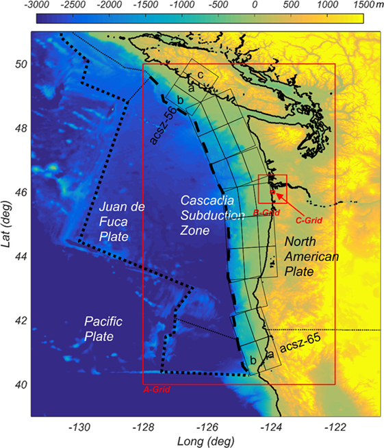
Figure 4. Cascadia subduction zone (CSZ) formed by the Juan de Fuca Plane and the North American Plate. The red boxes indicate the nested grids used in the tsunami modeling. The rectangular boxes along the CSZ show the slip locations used in the tsunami generation model and in the prediction of the ground-motion intensities. The study area of Seaside, Oregon, is located in the C-Grid.

Seaside, Oregon, is the study area chosen to demonstrate the proposed PSTHA methodology. Figure 5A shows an aerial view of Seaside with approximately 4 km of shoreline facing the Pacific Ocean and two small rivers, the Necanicum River and Neawanna Creek, that run parallel to the shoreline. The city has a population of approximately 6,500 residents, and the number of people in the city can increase to over 20,000 during the summer tourist season. There are over 5,700 buildings in Seaside with the larger hotels constructed out of steel and reinforced concrete in the center of the city (highlighted by the red box in Figure 5A) and surrounded by mostly wooden residential structures to the north and south of the city center. Figure 5B shows the bathymetry and topography of the study area. The remnant coastal dune on which the city was built can be seen running parallel to the shoreline with a secondary rise between the Necanicum River and Neawanna Creek. To the east of the Neawanna Creek, there is a steep gradient leading to the foot hills and a large headland to the south west. Figure 5C shows the distribution of the soil classes for this region. The steeper mountain areas are considered as Class C, and a majority of the city area is Class D (ASCE, 2010). The soil class distribution is also aligned approximately in the shore parallel direction.

FIGURE 5

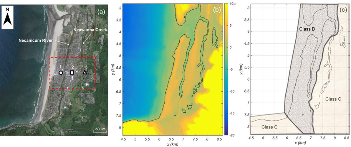
Figure 5. Study area of Seaside, Oregon, at the landward side of the C-Grid shown in Figure 4. (A) Satellite image of the City of Seaside area with Necanicum River and Neawanna Creek bisecting the city. Areas marked by 1 (circle), 2 (square), and 3 (triangle) are example locations used in later figures. Red box highlights detailed area in later figures. (B) Bathymetry/topography for study area. Note that waterfront area of the city is built on a remnant dune and has higher elevation than river areas. (C) Soil classes assumed based on DOGAMI Oregon Department of Geology and Mineral Industries (2017) maps.

Seaside has been the subject of multiple tsunami studies in the past because it is considered to be one of the most vulnerable locations to a CSZ event. As reported by Wood et al. (2010), the low lying city has approximately 87% of its land within the inundation zone of a CSZ full-rupture event, and 89% of the employees work within this zone. Because of the high vulnerability of Seaside to a CSZ event, there have been several recent studies in this area as reviewed by Park and Cox (2016) and Park et al. (2017), including the work by González et al. (2009) that conducted a PTHA using 14 historic tsunami far-field scenarios and 12 scenarios of the CSZ event.

CSZ Fault Modeling

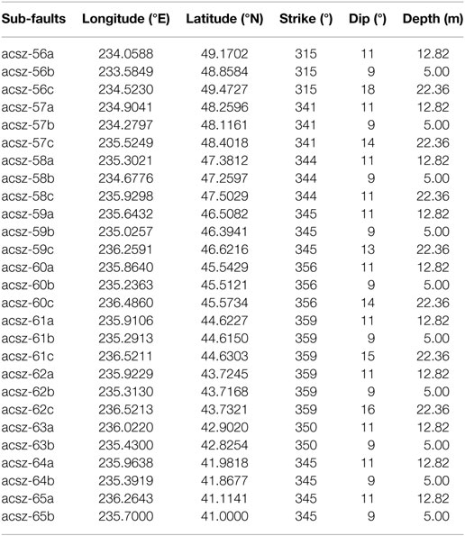
Figure 6 shows the logic-tree model utilized for both earthquake and tsunami for CSZ full-rupture event (Park and Cox, 2016). This logic-tree model characterizes the randomness of the fault slip in terms of the moment magnitude, peak slip location, and a fault slip shape. To simplify the scenarios, 27 sub-faults distributed along the CSZ were considered, which are the default sub-fault setup for the ComMIT model (Titov et al., 2011). The sub-faults are distributed from the northern Vancouver Island to Northern California. Each sub-fault is 100 km long by 50 km wide, as shown in Figure 4. The detailed geologic information of the location and slip information is summarized in Table 1. Each of the 27 sub-faults has a constant rake of 90° and has varied strike, dip, and depth conditions along the entire fault. The x and y coordinates indicate the middle point on the right edge boundary of each sub-faults in Figure 4.

FIGURE 6

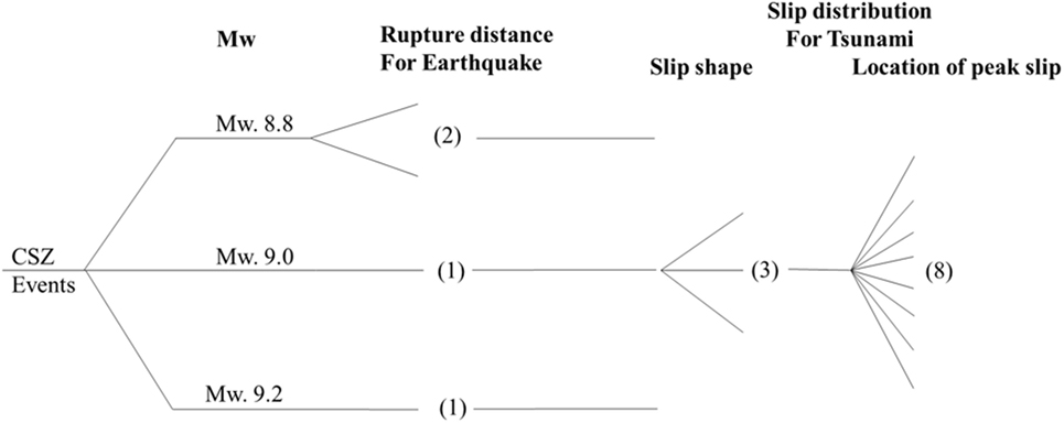
Figure 6. Logic-tree model for full-rupture event at Cascadia subduction zone (CSZ). Each number in parenthesis provides the number of branches (scenario cases) considered depending on the characteristics of the rupture events (see details in the study by Park and Cox, 2016).

TABLE 1

Table 1. Geologic sub-faults information at Cascadia subduction zone.

The full-rupture event at the CSZ is discretized as three moment magnitude scenarios (M 8.8, 9.0, and 9.2), and the corresponding rupture areas (S) were estimated using the relationship between seismic moment M₀ and rupture area provided by Murotani et al. (2013) and given by

$S=1.34\times {10}^{-10}{M}_0^{2/3}$ (17)

Park and Cox (2016) added upper and lower limits to the surface area moment magnitude relationships of Eq. 17 by multiplying Eq. 17 with 2.0 and 0.5, respectively, and these limits bounded most of historic recent tsunami events at SZ around the Pacific Ocean which are generated by earthquake scenarios with M > 8.5. Including those two limits, a total of three slip shapes along the strike direction were utilized as possible scenarios per moment magnitude condition. Additionally, 8 possible peak locations are considered along the rupture length, giving rise to 24 scenarios applied for each moment magnitude condition. A total of 72 scenarios (3 moment magnitudes × 3 slip shapes × 8 peak slip locations) are proposed here to characterize the full-rupture CSZ event. Park and Cox (2016) applied 72 scenarios as inputs to the ComMIT/MOST (Titov et al., 2011) model, which considers the elastic dislocation model (Okada, 1985) for tsunami generation and solves the non-linear shallow water equations implemented with a finite difference scheme. The ComMIT/MOST model consists of three nested grids (A, B, and C-Grid) shown in Figure 4. For the inundation modeling, the results of COULWAVE (Lynett et al., 2002) were used, which solves a set of Boussinesq equations with a high-order finite-volume method by using the output of ComMIT/MOST modeling at B-Grid as the input of COULWAVE at C-Grid. All bathymetry data were originated from NOAA’s National Geophysical Data Center and the DEM for the Seaside area whose resolution is 1/3 arc second was used for the C-Grid. Each A, B, and C-Grids has 1 min (400 × 400), 3 s (800 × 800), and 24 m (416 × 390) resolutions. As a tide condition, the mean high water level was fixed as conservative tsunami hazards estimation in this study. The model results provide surface elevation and velocity time series over the entire study area at the 24 m grid resolution. More details of fault slip distributions and tsunami simulations are available in the study by Park and Cox (2016). In case of earthquakes, the same fault model is used. However, the BC Hydro GMPE is utilized in this study, which is based on the closest rupture distance, R_rup, between the site of interest and rupture surface for the interface earthquakes considered.

Results

Seismicity

Though larger magnitude earthquakes generally have higher damage potential compared to smaller magnitude earthquakes, smaller and frequent events can be dominant contributors to the structural damage risk measured in terms of mean annual frequency of exceeding a damage state such as the collapse damage state (e.g., Zareian and Krawinkler, 2007; Eads et al., 2013). Figure 7A shows the probability mass function (PMF) of the earthquakes in CSZ deemed capable of generating tsunamis. Tsunamigenic eartquakes with lowest magnitude of m_min = 7.3 is assumed and largest magnitude is assumed to be m_max = 9.3, consistent with the earthquake expected over a 10,000-year period in CSZ (Rong et al., 2014). A discretization interval of Δm = 0.2 is adopted to develop the PMF of Figure 7, resulting in 10 central magnitude values m = 7.4 to m = 9.2. The PMF for different magnitudes are computed based on the TGR distribution described in Section “Earthquake Fault Source Models and Their Characteristics” and using Eq. 8. Of these 10 magnitudes, m ≥ 8.8 is assumed to produce the full rupture along the CSZ following the recommendations by Goldfinger et al. (2012), which is also consistent with Park and Cox (2016). These full-rupture events (m = 8.8, 9.0, 9.2) are only considered for earthquake-tsunami hazard analysis for Seaside. According to Figure 7A, λ_m≥8.8 = 0.002 results in 500-year return period for m ≥ 8.8 representing full-rupture scenarios. To be consistent with 526-year return period used in Park and Cox (2016) for full-rupture CSZ events, λ_m≥8.8 = 0.0019 is used for the PSHA computations for the study area of City of Seaside.

FIGURE 7

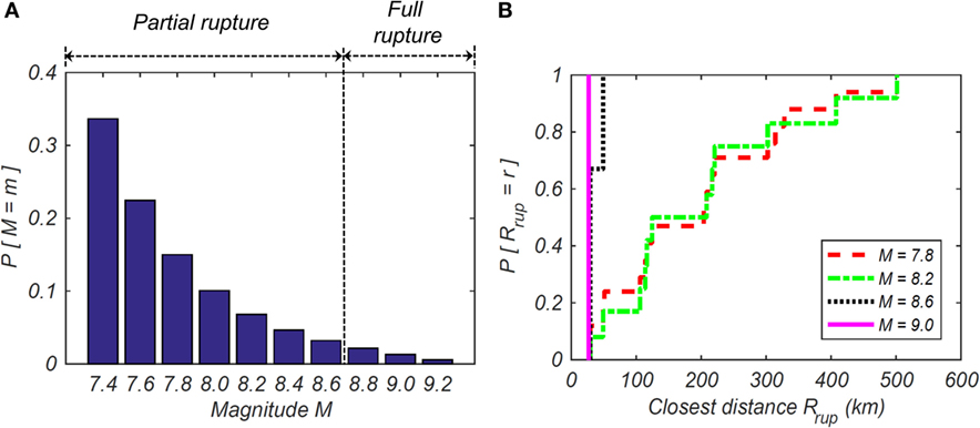
Figure 7. Probability mass function (PMF) of the ground-motion basic random variables for different earthquake scenarios computed for observation Point 1 based on the Tapered Gutenberg–Richter recurrence relationship: (A) PMF of the magnitude and (B) PMF of closest rupture distance.

One of the inputs required in the GMPEs for computing ground-motion intensities at a given site is the source-to-site distance. The BC Hydro GMPE used in this study is based on the closest rupture distance R_rup between the site of interest and the rupture surface for interface SZ earthquakes. To compute the R_rup for different locations in Seaside for different magnitude scenarios, the R_rup for all the C-grid locations are precomputed from the 27 sub-fault areas shown in Figure 4. The rupture surface for different magnitude scenarios of Figure 7A are then computed based on the magnitude scaling law by Murotani et al. (2013), which are randomly positioned along the 27 sub-faults corresponding to the approximately 1,000 km long by 150 m width fault plane. The randomly positioned rupture surfaces corresponding to different scenarios are subsequently used to interpolate the R_rup for each scenario from the precomputed closest distances. Figure 7B shows the PMF of R_rup computed for observation point 1 in Figure 5A. The closest distance computed for all the scenarios is 27.5 km, which is the distance computed from the fault area immediately below the C-grid. It can be observed in Figure 7B that smaller variability of R_rup is observed for larger magnitudes. For example, for m = 9.0 that is a full-rupture event results in a single source-to-site distance and the resulting R_rup can be considered as a deterministic event with P[R_rup = 27.5 km] = 1. For the partial rupture events, the rupture surface is randomly positioned within the fault plane, which results in variability in the closest rupture distance computed as shown in Figure 7B.

AEP for two earthquake IMs, PGA and S_a(T₁ = 0.3 s), are computed for three observation points (shown in Figure 5A) in Seaside. These points are aligned shore-normal along the urban center of Seaside with approximately 400 m distance apart from each other. The observation Points 1, 2, and 3 are located between shoreline and the Necanicum River, Necanicum River and the Neawanna Creek, and Neawanna Creek and the edge of inundation zone, respectively.

Figure 8 shows the AEP of PGA and S_a(T₁ = 0.3 s) at three observation points computed for the full-rupture scenarios (M = 8.8,M = 9.0,M = 9.2) using the BC Hydro GMPE. As per the soil site class map of Figure 5C, point 1 and point 2 fall in site class D where as point 3 is in site class C. The V_s30 values assigned to Point 1, Point 2, and Point 3 are 300, 360, and 420 m/s, respectively. A value of λ_m = 0.0019 corresponding to M ≥ 8.8 is used for the hazard curves and subsequent AEP computations. In AEP computations, the PMF values considered for the three magnitudes is consistent with those used in the study by Park and Cox (2016), which were obtained from the study by Goldfinger et al. (2012). Since the weights assigned to the M 8.8, M 9.0, and M 9.2 are 5/19, 13/19, and 1/19, respectively, the M 9.0 is the dominant contributor to the hazard curves presented in Figure 8 for both PGA and S_a(T₁ = 0.3 s), followed by M 8.8, and M 9.2, respectively. As shown in Figure 8, AEP of PGA for three points are almost identical whereas slight variation in AEP for S_a(T₁ = 0.3 s) is observed for those three points. The slight variation in AEP for S_a(T₁ = 0.3 s) is due to the different V_s30 values assigned to those points. Overall AEP of both IMs are insensitive to their geographical conditions at this 800 m distance between the three points, which are all approximately 27.5 km from the fault.

FIGURE 8

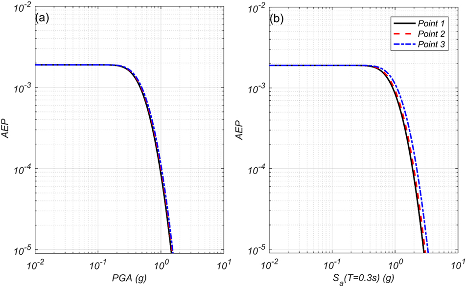
Figure 8. Annual exceedance probability (AEP) for peak ground acceleration (PGA) (A) and S_a(T₁ = 0.3 s) (B) at Points 1 (black solid), 2 (red dash), and 3 (blue dash-dot) for the full-rupture scenarios.

The joint MAR of exceedance of IMs contour plot of PGA and S_a(T₁ = 0.3 s) is shown in Figure 9 for the three points indicated in Figure 5 for the 1,000-year event. The joint MAR of exceedance of IMs is computed based on the formulation presented in Eqs 15 and 16, in which the joint probability function of the two IMs conditional on the magnitude at a given site is computed assuming that the IMs follow a joint lognormal distribution. For the jont MAR of exceedance computation of PGA and S_a(T₁ = 0.3 s), correlation between the two IMs are considered and computed based on the study by Baker and Jayaram (2008). It can be seen from Figure 9 that for all three observation points, the most likely joint intensities occur for values of PGA = 0.5 g and S_a(T₁ = 0.3 s) = 1.0 g. Moreover, there is no discernable difference in the joint hazard intensities among the observation points considered as can be observed in Figure 9, as expected.

FIGURE 9

Figure 9. Joint hazard curves of peak ground acceleration (PGA) and S_a at (A) Point 1, (B) Point 2, and (C) Point 3.

Tsunami Intensity

Figure 10 shows the AEP of two tsunami IMs h_max and (M_F)_max at the three observation points similar to Figure 8. Generally, the tsunami IMs decrease as distance from the shoreline increases because of the dissipation of energy during the inundation process as shown for the AEP of h_max (Figure 10A) and (M_F)_max (Figure 10B). For example, the AEP of both h_max and (M_F)_max at Point 1 are higher than Points 2 and 3. However, for lower probability events in the range of 0 < h_max ≤ 3 m, Points 2 and 3 have nearly the same AEP. Point 3 has higher h_max at the higher probability events in the range of 3 < h_max ≤ 10 m and also has the highest h_max due to the local topographic effects, including effects of the river and the creek running parallel to the shoreline (Figure 5A), highlighting the sensitivity of the tsunami IM to site-specific conditions. On the other hand, (M_F)_max shown in Figure 10B has three distinct curves with a generally decreasing trend from the shoreline to inundation limits. Comparing Figures 8 and 10, it is noted that the variation of AEP of tsunami IMs among three observation points are qualitatively dissimilar to the results of earthquakes IMs in that there are strong spatial gradients for the tsunami IMs across the length scale of the city. This is somewhat expected because the AEP of both PGA and S_a(T₁ = 0.3 s) depend primarily on the soil types and R_rup that have relatively small variations over the study region at Seaside, especially for the full-rupture scenarios considered. Moreover, this difference underscores the differences in the fundamental physics of the propagation of the seismic energy through the subsurface and the propagation of the hydrodynamic tsunami energy.

FIGURE 10

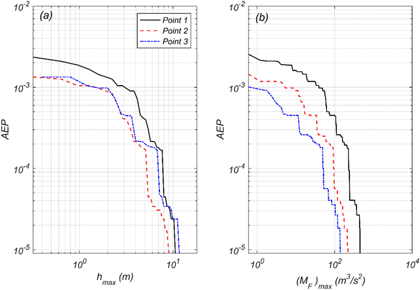
Figure 10. Annual exceedance probability (AEP) of h_max (A) and (M_F)_max (B) at Points 1 (black solid), 2 (red dash), and 3 (blue dash-dot).

Figures 11A–C shows the joint AEP of h_max and (M_F)_max at Point 1, 2, and 3, respectively, where the same number of bins for both IMs are utilized to calculate the vector-valued IMs of the joint h_max and (M_F)_max from Eqs 15 and 16. Figure 11 also includes the isolines for four Froude numbers (Fr = 0.2, 0.5, 1.0, and 2.0) to show the possible range of distributions of velocity fields at the given flow depth. In general, the results show the high correlation between h_max and (M_F)_max at all three observation points, and each joint AEP follows a particular Fr for that area. For example, at Point 1 when h_max is in the range 6 < h_max < 7 m, the corresponding range of (M_F)_max is 150 < (M_F)_max < 200 m³/s² and corresponds to a Fr range of approximately 0.6 < Fr < 0.7. The Fr generally decreases shoreward, and seems to be everywhere subcritical (Fr < 1.0) which is physically realistic based on observed inundations following the 2011 Tohoku tsunami. This is not to say that the flow is always subcritical, just that at the point of maximum flow depth or momentum flux, that the flow can be expected to be subcritical.

FIGURE 11

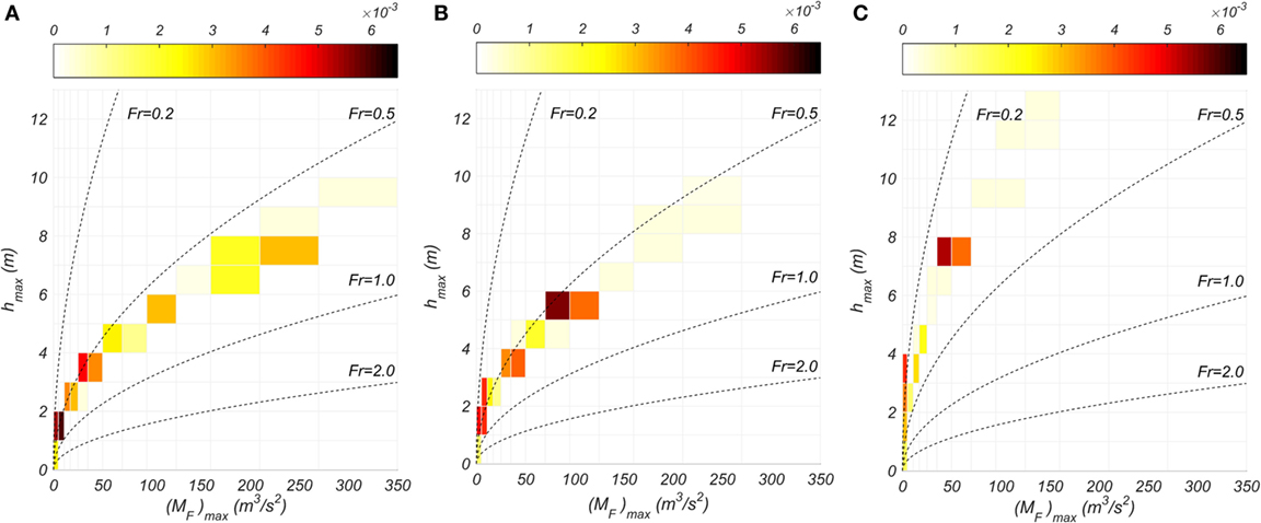
Figure 11. Joint MAR of h_max and (M_F)_max with Froude number (Fr) (dash lines) at (A) Point 1, (B) Point 2, and (C) Point 3.

Figure 11 reveals that the different distributions of the joint surface of the AEP following the specific Fr at three observation points originate from the local bathymetric/topographic conditions and not from the fault slip distributions. These results are helpful to understand realistic input conditions of flow depth and velocity fields for different Fr regime that can be used to develop the tsunami fragility curves, which utilize the random combinations of h_max and flow velocity in the generation of fragility curves (Attary et al., 2017a; Attary et al., 2017b; Alam et al., submitted²). In addition, it is worth noting that the maximum flow depth and momentum flux typically do not occur at the same time (Park et al., 2013). Therefore, Fr at the maximum momentum flux and at the maximum flow depth can be expected to be slightly different. However, plots similar to Figure 11 (not shown in the interest of brevity) in which the flow depth h at the instant of the maximum momentum flux (M_F)_max or the instantaneous momentum flux is plotted against the corresponding maximum inundation flow depth lead to similar conclusions that the flow is generally subcritical for the maximum IMs.

Spatial Representations Seismic and Tsunami Hazard

Figure 12 shows the spatial distributions of the earthquake and tsunami IMs at Seaside, Oregon, for the AEP = 0.001 (often referred to as the “1,000-year event”) for the full-rupture scenario at CSZ. Figures 12A–D presents the spatial distribution of PGA, S_a (T₁ = 0.3 s), h_max, and (M_F)_max respectively, and the dotted contour lines in each panel show the maximum inundation limits (h_max = 0.3 m). Two distinct regions of earthquake IMs (PGA and S_a) are observed for the study area depending on the soil site class assumed in Figure 5C and within each region distributions of IMs are generally uniform. In the case of tsunami IMs (h_max and (M_F)_max), irregular distributions are observed depending on the bathymetry conditions. However, both the IMs generally decreases from the shore toward inland (i.e., in the positive x-direction).

FIGURE 12

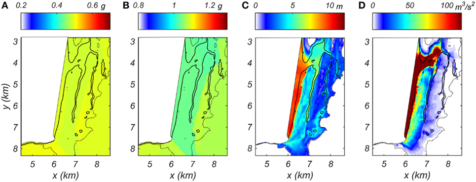
Figure 12. Spatial hazard maps of (A) peak ground acceleration, (B) S_a(T₁ = 0.3 s), (C) h_max, and (D) (M_F)_max for 1,000-year event.

The range of PGA and S_a(T₁ = 0.3 s) over the study region is 0.47–0.50 g and 1.03–1.08 g, respectively, while the h_max and (M_F)_max range from 0 to 12 m and 0 to 120 m³/s², respectively for the 1,000-year event. The values of PGA and S_a are uniformly distributed over the entire study area, while the area affected by h_max and (M_F)_max are limited to the maximum inundation limits. To understand the granularity of both IMs of the earthquake and tsunami at the same event, the spatial mean and deviation of IMs conditional on varying unit block size is computed. This analysis is performed on the rectangle region, shown in Figure 5A, which is a 1,990 m length and 3,000 m wide rectangle near the center of the City of Seaside. The smallest unit block size, designated as reference or unit block size here forth, is equal to the Cartesian mesh grid size (dx = dy = 24 m) considered for tsunami inundation modeling in the C-grid. The ratio of block size $\left(r_B=\frac{\text{Block }\mathit{size}}{\text{reference mesh size}}\right)$ is increased systematically, keeping the same block shape and the mean and SD of the IMs are estimated as a function of the changes in the block size. The mean of normalized IM is given by

${\mathit{IM}}^{\prime }=\frac{{\displaystyle \sum _{j=1}^{N_b}}\left({\displaystyle \sum _{i=1}^{N_g}}{\mathit{im}}_{i,j}^{\prime }\right)}{N_b{N}_g}$ (18)

where N_b is the number of blocks depending on r_B conditions, and N_g is the number of grid points in a jth block (N_g = r_B²). The ${\mathit{im}}_{\mathit{ij}}^{\prime }$ is the normalized IM of grid points of the jth block. The IMs in the jth block are normalized by the mean of the IMs for the jth blocks, and this calculation is performed for eight r_B conditions: r_B = 1, 2, 3, 5, 8, 13, 18, and 25. The corresponding block size and number of grid points per each block (N_g) are 24 m (1), 48 m (4), 72 m (9), 120 m (25), 192 m (64), 312 m (169), 432 m (324), and 600 m (625). For example, the total number of grid points in the study region is 10,625. For the case of r_B = 5, there are 425 block subsets over the study region, and each block is composed of N_g = 25 mesh grid points. The mean of IM at each of the 425 blocks is first computed, and then, each IM is normalized by the calculated mean.

Figure 13 shows the PDF of ln(h_max′) over the study region for AEP = 0.001 (1,000-year event). Figures 13A–D show the PDFs at r_B = 2, 5, 13, and 25, respectively. The red line in each panel shows the natural log-normal fitting curve. When ln(h_max′) is equal to zero, the mean of block subsets match exactly with the h_max of the unit grids, and each negative or positive value indicates an overestimation or underestimation of the block means. In the case of h_max, the PDF shape becomes wider and shows a larger deviation as the block size increases. This process was extended to the three other IMs: PGA and S_a and (M_F)_max.

FIGURE 13

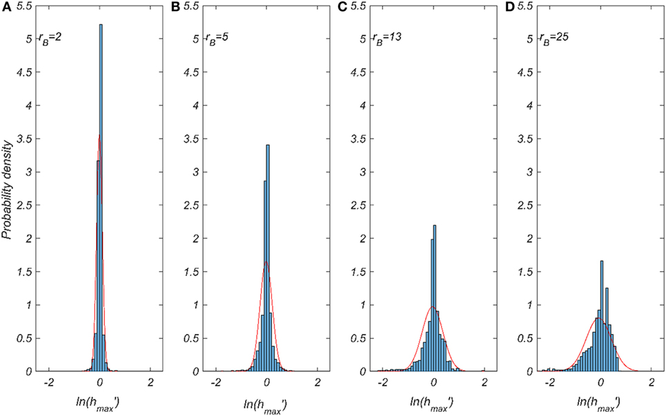
Figure 13. Probability density function (PDF) of normalized h_max for 1,000-year event. (A) r_B = 2, (B) r_B = 5, (C) r_B = 13, and (D) r_B = 25. Each red line in the panel shows the fitted natural lognormal PDF curves.

Figure 14 summarizes the results of the four granularity tests for AEP = 0.001 (1,000-year event) by plotting the mean of the four normalized IMs with 90% confidence intervals for each unit block size. Both PGA and S_a (T₁ = 0.3 s) show almost insensitivity to the block sizes. All of the normalized means are essentially zero and the confidence intervals are small for all block sizes. However, both h_max and (M_F)_max results show significant variation with the 90% confidence intervals increasing as the block size increases. The largest deviation is found at (M_F)_max, and relatively smaller deviation if found h_max. The range of confidence interval of both h_max and (M_F)_max increases sharply with r_B = 13 (block size = 312 m). These results highlight the different sensitivity between two earthquake and tsunami IMs to the block size used to aggregate the IM results. In case of the PGA and S_a, the information of the site and location are less significant for determining each IM while h_max and (M_F)_max require detailed information of the site to minimize the uncertainty.

FIGURE 14

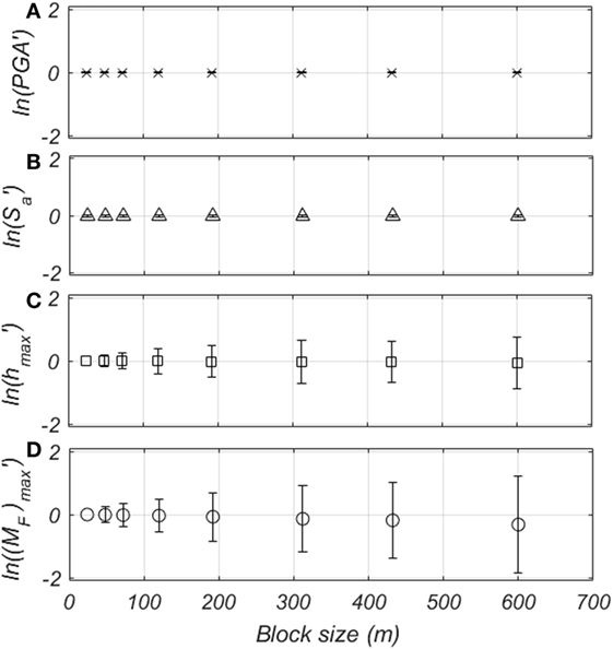
Figure 14. Granularity of (A) peak ground acceleration (PGA), (B) S_a(T₁ = 0.3 s), (C) h_max, and (D) (M_F)_max for 1,000-year event.

Lastly, the spatial distribution of joint IMs is analyzed next. Only h_max and (M_F)_max are considered herein since significant variations of tsunami IMs across the study area is observed in Figure 12. For the joint distribution computations uniform bins at 0.2 m interval are used for h_max, while a 4 m³/s² interval is used for (M_F)_max. The probability (%) of the joint distribution is computed by counting number of grids which involved in the joint h_max and (M_F)_max bin, for the whole study region, at the three AEP conditions, i.e., the 500, 1,000, and 2,500-year events, respectively. The results of spatial distributions of joint probability of h_max and (M_F)_max are shown in Figures 15A–C for the 500, 1,000, and 2,500-year events, respectively, with four Froude numbers plotted on each figure in a manner similar to Figure 11.

FIGURE 15

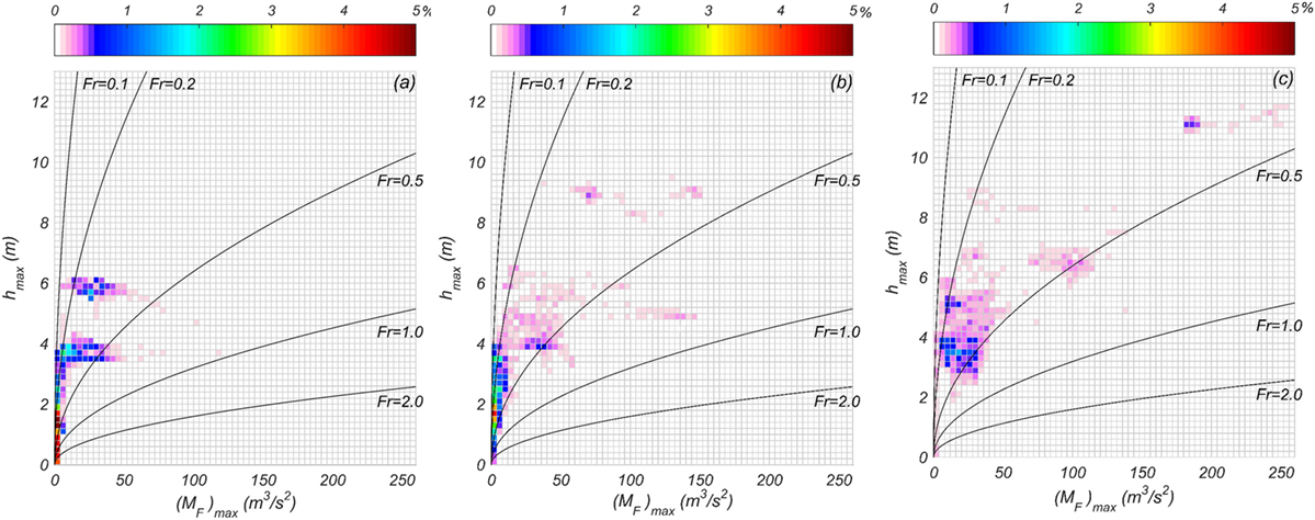
Figure 15. Spatial distribution of joint h_max and (M_F)_max with Froude number (Fr) for (A) 500, (B) 1,000, and (C) 2,500-year events.

In the case of the 500-year event (Figure 15A), more than 45% of the joint h_max and (M_F)_max is distributed within 0.1 < Fr ≤ 0.5. The larger (M_F)_max is observed within 0.5 < Fr ≤ 1.0. The joint peak of h_max and (M_F)_max is located at 1.2 < h_max ≤ 1.4 m, and 0.0 < (M_F)_max ≤ 4.0 m³/s². Two distinct narrow banded regions of h_max are observed near h_max = 3.8 and h_max = 5.8 m, which correspond to different ranges of (M_F)_max even at the similar flow depth conditions. In the case of the 1,000-year event (Figure 15B), more than 60% of the joint h_max and (M_F)_max is distributed within 0.1 < Fr ≤ 0.5. Large (M_F)_max values are observed at both 0.1 < Fr ≤ 0.5 and 0.5 < Fr ≤ 1.0. The joint peak is located at 1.6 ≤ h_max < 1.8 m, and 0.0 < (M_F)_max ≤ 4.0 m³/s² which is a slightly higher h_max condition than the 500-year event. Several isolated islands of joint distributions are observed that have relatively higher (M_F)_max values. In the case of the 2,500-year event (Figure 15C), more than 68% of the joint h_max and (M_F)_max is located within 0.1 < Fr ≤ 0.5. Large (M_F)_max values are located primarily within 0.1 < Fr ≤ 0.5. The joint peak is located at 3.4 < h_max ≤ 3.6 m, and 16.0 < (M_F)_max ≤ 20.0 m³/s², which are significantly larger than the 500 and 1,000-year events. A few isolated points are observed for 2500-year event similar to that observed in 1,000-year event. Overall, the joint h_max and (M_F)_max is distributed within 0.1 ≤ Fr < 1.0 and are typically in the range 0.1 < Fr ≤ 0.5. It is also observed that each event has a different joint peak location. Further research is needed to understand the extent to which these are site-specific results, how this work can be generalized for other coastal archetypes (e.g., embayments), and how these results can be parameterized based on conditions offshore of the study area.

Summary, Conclusion, and Future Work

This paper presents a framework for a consistent probabilistic hazard assessment for the multi-hazard seismic and tsunami phenomena (PSTHA). For this work, full-rupture event along the CSZ is considered and the PSTHA methodology is applied to the study area of Seaside, Oregon, along the US Pacific Northwest coast. In this work, it is shown that:

1. The AEPs off the tsunami IMs are qualitatively dissimilar to the IMs of the seismic ground motion in the study area. Specifically, the spatial gradients for the tsunami IMs are much stronger across the length scale of the city owing to the physical differences of energy dissipation of the two mechanisms.

2. For the seismic hazard, similar trends were observed for the joint MAR of exceedance of the PGA and S_a(T₁ = 0.3 s) at the three observation points, which may be attributed to the proximity of the observation points with respect to each other as well as from the source of the meag-thrust full rupture of CSZ.

3. For the tsunami hazard, the joint AEP of h_max and (M_F)_max show a high correlation between h_max and (M_F)_max in the study area. The joint AEP at each of the three observation points follows a particular Fr due to the local site-specific conditions at each location rather than the distributions of fault slips.

4. The joint probability distribution of h_max and (M_F)_max throughout the study region falls between 0.1 ≤ Fr < 1.0 (i.e., the flow is subcritical), regardless of return interval (500-, 1,000-, and 2,500-year). However, the peak of the joint probability distribution with respect to h_max and (M_F)_max varies with the return interval, and the largest values of h_max and (M_F)_max were observed with the highest return intervals (2,500 year) as would be expected.

The tsunami inundation simulations were conducted with a bare earth DEM, and the effects of the natural and built environment were simply modeled using a single friction factor. It is known that the tsunami inundation velocity is sensitive to the choice of friction factor (e.g., Park et al., 2013) and that the friction factor can vary significantly for the built environment (e.g., Bricker et al., 2015). Therefore, future research should consider the effect of bottom friction uncertainty in modeling the probabilistic tsunami hazard assessment. Moreover, the difference in the types of models being used with respect to the approximation of the governing equations (e.g., non-linear shallow water equations or Boussinesq equations), solution techniques (finite element, finite difference), grid resolution, and so on introduce model source uncertainty and should be evaluated in a similar manner as bottom friction.

In terms of multi-hazards, future PSTHA frameworks should include additional sources such as other earthquake faults (on land), which would not produce tsunamis. Nonetheless, these would contribute to the seismic hazard in the region. Conversely, distance sources tsunamis should also be included, which may not produce ground shaking.

The results of the PSTHA can be the basis for a probabilistic multi-hazard damage assessment (PTSDA) to quantify the separate contributions of seismicity and tsunami hazards in the estimation of damage to the built environment over the community scale. In addition, it will be necessary to understand the propagation of uncertainties of the hazard assessments combined with the uncertainties of the damage estimates to evaluate the overall community risk to the multi-hazards. Moreover, the PTSDA should be evaluated considering the spatial gradients of the building damages at a community scale due to the site information (e.g., building types) or fragility functions applied to each building for both earthquake and tsunami IMs across the length scale.

Author Contributions

Each author contributed equally to the manuscript. HP and DC contributed to the tsunami hazard modeling. MA and AB contributed to the seismic hazard modeling.

Conflict of Interest Statement

The authors declare that the research was conducted in the absence of any commercial or financial relationships that could be construed as a potential conflict of interest.

Funding

Funding for this study was provided as part of the cooperative agreement 70NANB15H044 between the National Institute of Standards and Technology (NIST) and Colorado State University through a subaward to Oregon State University. The content expressed in this paper are the views of the authors and do not necessarily represent the opinions or views of NIST or the U.S. Department of Commerce.

Footnotes

1. ^Mori, N., Goda, K., and Cox, D. T. (submitted). “Recent progress in probabilistic tsunami hazard analysis (PTHA) for mega thrust subduction earthquakes,” in Reconstruction and Restoration after the 2011 Japan Earthquake and Tsunami (Springer).
2. ^Alam, M. S., Barbosa, A. R., Scott, M. H., Cox, D., and van de Lindt, J. W. (submitted). Development of physics-based tsunami fragility functions considering structural member failures. ASCE J. Struct. Eng.

References

Abrahamson, N., Gregor, N., and Addo, K. (2016). BC Hydro ground motion prediction equations for subduction earthquakes. Earthq. Spectra 32, 23–44. doi:10.1193/051712EQS188MR

CrossRef Full Text | Google Scholar

Anita, G., Sandri, L., Marzocchi, W., Argnani, A., Gasparini, P., and Selva, J. (2012). Probabilistic tsunami hazard assessment for Messina Strait Area (Sicily, Italy). Nat. Hazards 64, 329–358. doi:10.1007/s11069-012-0246-x

CrossRef Full Text | Google Scholar

Annaka, T., Satake, K., Sakakiyama, T., Yanagisawa, K., and Shuto, N. (2007). Logic-tree approach for probabilistic tsunami hazard analysis and its applications to the Japanese coasts. Pure appl. geophys. 164, 577–592. doi:10.1007/s00024-006-0174-3

CrossRef Full Text | Google Scholar

ASCE. (2010). ASCE 7-10 Minimum Design Loads for Buildings and Other Structures. Reston, VA: American Society of Civil Engineering.

Google Scholar

Atkinson, G. M., Assatourians, K., Boore, D. M., Campbell, K., and Motazedian, D. (2009). A guide to differences between stochastic point-source and stochastic finite-fault simulations. Bull. Seismol. Soc. Am. 99, 3192–3201. doi:10.1785/0120090058

CrossRef Full Text | Google Scholar

Atkinson, G. M., and Boore, D. M. (2003). Empirical ground-motion relations for subduction-zone earthquakes and their application to Cascadia and other regions. Bull. Seismol. Soc. Am. 93, 1703–1729. doi:10.1785/0120020156

CrossRef Full Text | Google Scholar

Atkinson, G. M., and Boore, D. M. (2008). Erratum to empirical ground-motion relationships for subduction-zone earthquakes and their application to Cascadia and other regions. Bull. Seismol. Soc. Am. 98, 2567–2569.

Google Scholar

Atkinson, G. M., Goda, K., and Assatourians, K. (2011). Comparison of nonlinear structural responses for accelerograms simulated from the stochastic finite-fault approach versus the hybrid broadband approach. Bull. Seismol. Soc. Am. 101, 2967–2980. doi:10.1785/0120100308

CrossRef Full Text | Google Scholar

Attary, N., van de Lindt, J. W., Unnikrishnan, V. U., Barbosa, A. R., and Cox, D. T. (2017a). Methodology for development of physics-based tsunami fragilities. J. Struct. Eng. doi:10.1061/(ASCE)ST.1943-541X.0001715

CrossRef Full Text | Google Scholar

Attary, N., Unnikrishnan, V. U., van de Lindt, J. W., Cox, D. T., and Barbosa, A. R. (2017b). Performance-based tsunami engineering methodology for risk assessment of structures. Eng. Struct. 141, 676–686. doi:10.1016/j.engstruct.2017.03.071

CrossRef Full Text | Google Scholar

Atwater, B. F., and Griggs, G. B. (2012). “Deep-sea turbidites as guides to holocene earthquake history at the Cascadia subduction zone,” in Alternative Views for a Seismic-Hazard Workshop: U.S. Geological Survey Open-File Report 2012–1043, Seattle, WA, 58.

Google Scholar

Baker, J. W. (2011). Conditional mean spectrum: tool for ground-motion selection. J. Struct. Eng. 137, 322–331. doi:10.1061/(ASCE)ST.1943-541X.0000215

CrossRef Full Text | Google Scholar

Baker, J. W., and Jayaram, N. (2008). Correlation of spectral acceleration values from NGA ground motion models. Earthq. Spectra 24, 299–317. doi:10.1193/1.2857544

CrossRef Full Text | Google Scholar

Barbosa, A. R. (2011). Simplified Vector-Valued Probabilistic Seismic Hazard Analysis and Probabilistic Seismic Demand Analysis: Application to the 13-Story NEHRP Reinforced Concrete Frame-Wall Building Design Example. Ph.D. Dissertation, University of California San Diego, California.

Google Scholar

Bazzurro, P. (1998). Probabilistic Seismic Demand Analysis. Ph.D. Dissertation. Stanford University, California.

Google Scholar

Benjamin, J. R., and Cornell, C. A. (1970). Probability, Statistics, and Decision for Civil Engineers. New York: McGraw-Hill.

Google Scholar

Bird, P., and Kagan, Y. Y. (2004). Plate-tectonic analysis of shallow seismicity: apparent boundary width, beta, corner magnitude, coupled lithosphere thickness, and coupling in seven tectonic settings. Bull. Seismol. Soc. Am. 94, 2380–2399. doi:10.1785/0120030107

CrossRef Full Text | Google Scholar

Bricker, J. D., Gibson, S., Takagi, H., and Imamura, F. (2015). On the need for larger manning’s roughness coefficients in depth-integrated tsunami inundation models. Coast. Eng. J. 57, 1550005. doi:10.1142/S0578563415500059

CrossRef Full Text | Google Scholar

Burbidge, D., Cummins, P. R., Mleczko, R., and Thio, H. K. (2008). A probabilistic tsunami hazard assessment for Western Australia. Pure appl. geophys. 165, 2059–2088. doi:10.1007/s00024-008-0421-x

CrossRef Full Text | Google Scholar

Burroughs, S. M., and Tebbens, S. F. (2005). Power-law scaling and probabilistic forecasting of tsunami runup height. Pure Appl. Geophys. 162, 331–342. doi:10.1007/s00024-004-2603-5

CrossRef Full Text | Google Scholar

Cornell, C. A. (1968). Engineering seismic risk analysis. Bull. Seismol. Soc. Am. 58, 1583–1606.

Google Scholar

Crouse, C. B. (1991). Ground-motion attenuation equation for earthquake on Cascadia Subduction-Zone earthquake. Earthq. Spectra 7, 210–236. doi:10.1193/1.1585626

CrossRef Full Text | Google Scholar

Crouse, C. B., Yogesh, K. V., and Schell, B. A. (1988). Ground motions from subduction zone earthquakes. Bull. Seismol. Soc. Am. 78, 1–25.

Google Scholar

De Risi, R., and Goda, K. (2016). Probabilistic earthquake–tsunami multi-hazard analysis: application to the Tohoku Region, Japan. Front. Built Environ. 2:25. doi:10.3389/fbuil.2016.00025

CrossRef Full Text | Google Scholar

Delorey, A. A., Frankel, A. D., Liu, P., and Stephenson, W. J. (2014). Modeling the effects of source and path heterogeneity on ground motions of great earthquakes on the Cascadia subduction zone using 3D simulations. Bull. Seismol. Soc. Am. 104, 1430–1446. doi:10.1785/0120130181

CrossRef Full Text | Google Scholar

DOGAMI Oregon Department of Geology and Mineral Industries. (2017). Oregon HazVu: Statewide Geohazards Viewer. Available at: http://www.oregongeology.org/sub/hazvu/

Google Scholar

Douglas, J. (2003). Earthquake ground motion estimation using strong-motion records: a review of equations for the estimation of peak ground acceleration and response spectral ordinates. Earth Sci. Rev. 61, 43–104. doi:10.1016/S0012-8252(02)00112-5

CrossRef Full Text | Google Scholar

Douglas, J. (2011). Ground-Motion Prediction Equations 1964-2010. Berkeley, CA: Pacific Earthquake Engineering Research Center, 444.

Google Scholar

Douglas, J. (2016). Ground-Motion Prediction Equations 1964-2016. 564. Available at: http://gmpe.org.uk/gmpereport2014.pdf

Google Scholar

Douglas, J., and Edwards, B. (2016). Recent and future developments in earthquake ground motion estimation. Earth Sci. Rev. 160, 203–219. doi:10.1016/j.earscirev.2016.07.005

CrossRef Full Text | Google Scholar

Eads, L., Miranda, E., Krawinkler, H., and Lignos, D. G. (2013). An efficient method for estimating the collapse risk of structures in seismic regions. Earthq. Eng. Struct. Dyn. 42, 25–41. doi:10.1002/eqe.2191

CrossRef Full Text | Google Scholar

Faggella, M., Barbosa, A. R., Conte, J. P., Spacone, E., and Restrepo, J. I. (2013). Probabilistic seismic response analysis of a 3-D reinforced concrete building. Struct. Safety 44, 11–27. doi:10.1016/j.strusafe.2013.04.002

CrossRef Full Text | Google Scholar

Frankel, A., Chen, R., Petersen, M., Moschetti, M., and Sherrod, B. (2015). 2014 update of the Pacific northwest portion of the US national seismic hazard maps. Earthq. Spectra 31, S131–S148. doi:10.1193/111314EQS193M

CrossRef Full Text | Google Scholar

Frankel, A., Paul, T., and Rohay, A. (2014). Three-Dimensional Ground-Motion Simulations of Earthquakes for the Hanford Area, Washington. U.S. Geological Survey Open-File Report 2013–1289, Reston, VA, 48.

Google Scholar

Fukutani, Y., Suppasri, A., and Imamura, F. (2015). Stochastic analysis and uncertainty assessment of tsunami wave height using a random source parameter model that targets a Tohoku-type earthquake fault. Stoch. Environ. Res. Risk Assess. 29, 1763–1779. doi:10.1007/s00477-014-0966-4

CrossRef Full Text | Google Scholar

Geist, E. L., and Parsons, T. (2006). Probabilistic analysis of tsunami hazards. Nat. Hazards 37, 277–314. doi:10.1007/s11069-005-4646-z

CrossRef Full Text | Google Scholar

Gidaris, I., Padgett, J., Barbosa, A. R., Chen, S., Cox, D., Webb, B., et al. (2016). Multiple-hazard fragility and restoration models of highway bridges for regional risk and resilience assessment in the U.S.: a state-of-the-art review. ASCE J. Struct. Eng. 143, 04016188-1–04016188-17. doi:10.1061/(ASCE)ST.1943-541X.0001672

CrossRef Full Text | Google Scholar

Goda, K., Mai, P. M., Yasuda, T., and Mori, N. (2014). Sensitivity of tsunami wave profiles and inundation simulations to earthquake slip and fault geometry for the 2011 Tohoku earthquake. Earth Planets Space 66, 1–20. doi:10.1186/1880-5981-66-105

CrossRef Full Text | Google Scholar

Goda, K., and Song, J. (2016). Uncertainty modeling and visualization for tsunami hazard and risk mapping: a case study for the 2011 Tohoku earthquake. Stoch. Environ. Res. Risk Assess. 30, 2271–2285. doi:10.1007/s00477-015-1146-x

CrossRef Full Text | Google Scholar

Goda, K., Yasuda, T., Mori, N., and Maruyama, T. (2016). New scaling relationships of earthquake source parameters for stochastic tsunami simulation. Coast. Eng. J. 58, 1650010. doi:10.1142/S0578563416500108

CrossRef Full Text | Google Scholar

Goldfinger, C., Nelson, C. H., Morey, A. E., Johnson, J. E., Patton, J. R., Karabanov, E., et al. (2012). “Turbidite event history: methods and implications for holocene paleoseismicity of the Cascadia subduction zone,” in U.S. Geological Survey Professional Paper 1661-F, Corvallis, OR, 178.

Google Scholar

González, F. I., Geist, E. L., Jaffe, B., Kânoglu, U., Mofjeld, H., Synolakis, C. E., et al. (2009). Probabilistic tsunami hazard assessment at seaside, Oregon, for near- and far-field seismic sources. J. Geophys. Res. Oceans 114, C11. doi:10.1029/2008JC005132

CrossRef Full Text | Google Scholar

Grezio, A., Marzocchi, W., Sandri, L., and Gasparini, P. (2010). A Bayesian procedure for probabilistic tsunami hazard assessment. Nat. Hazards 53, 159–174. doi:10.1007/s11069-009-9418-8

CrossRef Full Text | Google Scholar

Heaton, T. H., and Hartzell, S. H. (1987). Earthquake hazards on the Cascadia subduction zone. Science 236, 162–168. doi:10.1126/science.236.4798.162

PubMed Abstract | CrossRef Full Text | Google Scholar

Heidarzadeh, M., and Kijko, A. (2011). A probabilistic tsunami hazard assessment for the Makran subduction zone at the northwestern Indian Ocean. Nat. Hazards 56, 577–593. doi:10.1007/s11069-010-9574-x

CrossRef Full Text | Google Scholar

Iwaki, A., Maeda, T., Morikawa, N., Aoi, S., and Fujiwara, H. (2016). Kinematic source models for long-period ground motion simulations of megathrust earthquakes: validation against ground motion data for the 2003 Tokachi-oki earthquake. Earth Planets Space 68, 95. doi:10.1186/s40623-016-0473-6

CrossRef Full Text | Google Scholar

Jaffe, B. E., Borrero, J. C., Prasetya, G. S., Peters, R., McAdoo, B., Gelfenbaum, G., et al. (2006). Northwest Sumatra and offshore islands field survey after the December 2004 Indian Ocean tsunami. Earthq. Spectra 22, 105–135. doi:10.1193/1.2207724

CrossRef Full Text | Google Scholar

Kagan, Y. Y. (1997). Seismic moment-frequency relation for shallow earthquakes: regional comparison. J. Geophys. Res. Solid Earth 102, 2835–2852. doi:10.1029/96JB03386

CrossRef Full Text | Google Scholar

Kagan, Y. Y. (2002a). Seismic moment distribution revisited: I. Statistical results. Geophys. J. Int. 148, 520–541. doi:10.1046/j.1365-246x.2002.01594.x

CrossRef Full Text | Google Scholar

Kagan, Y. Y. (2002b). Seismic moment distribution revisited: II. Moment conservation principle. Geophys. J. Int. 149, 731–754. doi:10.1046/j.1365-246X.2002.01671.x

CrossRef Full Text | Google Scholar

Kramer, S. L. (1996). Geotechnical Earthquake Engineering. India: Pearson Education.

Google Scholar

Leonard, L. J., Rogers, G. C., and Mazzotti, S. (2014). Tsunami hazard assessment of Canada. Nat. Hazards 70, 237–274. doi:10.1007/s11069-013-0809-5

CrossRef Full Text | Google Scholar

Li, H., Yuan, Y., Xu, Z., Wang, Z., Wang, J., Wang, P., et al. (2016). The dependency of probabilistic tsunami hazard assessment on magnitude limits of seismic sources in the South China Sea and adjoining basins. Pure Appl. Geophys. 1–20.

Google Scholar

Lin, P. S., and Lee, C. T. (2008). Ground-motion attenuation relationships for subduction-zone earthquakes in northeastern Taiwan. Bull. Seismol. Soc. Am. 98, 220–240. doi:10.1785/0120060002

CrossRef Full Text | Google Scholar

Lin, T., Harmsen, S. C., Baker, J. W., and Luco, N. (2013). Conditional spectrum computation incorporating multiple causal earthquakes and ground-motion prediction models. Bull. Seismol. Soc. Am. 103, 1103–1116. doi:10.1785/0120110293

CrossRef Full Text | Google Scholar

Liu, Y., Santos, A., Wang, S. M., Shi, Y., Liu, H., and Yuen, D. A. (2007). Tsunami hazards along Chinese coast from potential earthquakes in South China Sea. Phys. Earth Planet. Inter. 163, 233–244. doi:10.1016/j.pepi.2007.02.012

CrossRef Full Text | Google Scholar

Lynett, P., Wu, T., and Liu, P. (2002). Modeling wave runup with depth-integrated equations. Coast. Eng. 46, 89–107. doi:10.1016/S0378-3839(02)00043-1

CrossRef Full Text | Google Scholar

Mas, E., Koshimura, S., Suppasri, A., Matsuoka, M., Matsuyama, M., Yoshii, T., et al. (2012). Developing tsunami fragility curves using remote sensing and survey data of the 2010 Chilean tsunami in Dichato. Nat. Hazards Earth Syst. Sci. 12, 2689–2697. doi:10.5194/nhess-12-2689-2012

CrossRef Full Text | Google Scholar

McGuire, R. K. (1995). Probabilistic seismic hazard analysis and design earthquakes: closing the loop. Bull. Seismol. Soc. Am. 85, 1275–1284.

Google Scholar

McGuire, R. K. (2004). Seismic Hazard and Risk Analysis. Berkeley, CA: Earthquake Engineering Research Institute, 240.

Google Scholar

Mori, N., Cox, D. T., Yasuda, T., and Mase, H. (2013). Overview of the 2011 Tohoku earthquake tsunami damage and its relation to coastal protection along the Sanriku coast. Earthq. Spectra 29, S127–S143. doi:10.1193/1.4000118

CrossRef Full Text | Google Scholar

Mueller, C., Power, W., Fraser, S., and Wang, X. (2015). Effects of rupture complexity on local tsunami inundation: implications for probabilistic tsunami hazard assessment by example. J. Geophys. Res. Solid Earth 120, 488–502.

Google Scholar

Murotani, S., Satake, K., and Fujii, Y. (2013). Scaling relations of seismic moment, rupture area, average slip, and asperity size for M 9 subduction-zone earthquakes. Geophys. Res. Lett. 40, 5070–5074. doi:10.1002/grl.50976

CrossRef Full Text | Google Scholar

Okada, Y. (1985). Surface deformation due to shear and tensile faults in a half-space. Bull. Seismol. Soc. Am. 75, 1135–1154.

Google Scholar

Olsen, K. B., Stephenson, W. J., and Geisselmeyer, A. (2008). 3D crustal structure and long-period ground motions from a M9.0 megathrust earthquake in the Pacific Northwest region. J. Seismol. 12, 145–159. doi:10.1007/s10950-007-9082-y

CrossRef Full Text | Google Scholar

Papazachos, B. C., Scordilis, E. M., Panagiotopoulus, C. B., and Karakaisis, G. F. (2004). Global relations between seismic fault parameters and moment magnitudes of earthquakes. Bull. Geol. Soc. Greece 36, 1482–1489.

Google Scholar

Park, H., and Cox, D. T. (2016). Probabilistic assessment of near-field tsunami hazards: inundation depth, velocity, momentum flux, arrival time, and duration applied to seaside, Oregon. Coast. Eng. 117, 79–96. doi:10.1016/j.coastaleng.2016.07.011

CrossRef Full Text | Google Scholar

Park, H., Cox, D. T., and Barbosa, A. (2017). Comparison of inundation depth and momentum flux based fragilities for probabilistic tsunami damage assessment and uncertainty analysis. Coast. Eng. 122, 10–26. doi:10.1016/j.coastaleng.2017.01.008

CrossRef Full Text | Google Scholar

Park, H., Cox, D. T., Lynett, P. J., Wiebe, D. M., and Shin, S. (2013). Tsunami inundation modeling in constructed environments: a physical and numerical comparison of free-surface elevation, velocity, and momentum flux. Coast. Eng. 79, 9–21. doi:10.1016/j.coastaleng.2013.04.002

CrossRef Full Text | Google Scholar

Power, W., Downes, G., and Stirling, M. (2007). Estimation of tsunami hazard in New Zealand due to South American Earthquakes. Pure Appl. Geophys. 164, 547–564. doi:10.1007/s00024-006-0166-3

CrossRef Full Text | Google Scholar

Power, W., Wang, X., Lane, E., and Gillibrand, P. (2013). A probabilistic tsunami hazard study of the Auckland region, part I: propagation modelling and tsunami hazard assessment at the shoreline. Pure Appl. Geophys. 170, 1621–1634. doi:10.1007/s00024-012-0543-z

CrossRef Full Text | Google Scholar

Priest, G. R., Goldfinger, C., Wang, K., Witter, R. C., Zhang, Y., and Baptista, A. M. (2010). Confidence levels for tsunami-inundation limits in northern Oregon inferred from a 10,000-year history of great earthquakes at the Cascadia subduction zone. Nat. Hazards 54, 27–73. doi:10.1007/s11069-009-9453-5

CrossRef Full Text | Google Scholar

Pulido, N., Aguilar, Z., Tavera, H., Chlieh, M., Calderon, D., Sekiguchi, T., et al. (2015). Scenario source models and strong ground motion for future mega-earthquakes: application to Lima, Central Peru. Bull. Seismol. Soc. Am. 105, 368–386. doi:10.1785/0120140098

CrossRef Full Text | Google Scholar

Rikitake, T., and Aida, I. (1988). Tsunami hazard probability in Japan. Bull. Seismol. Soc. Japan 78, 1268–1278.

Google Scholar

Rong, Y., Jackson, D. D., Magistrale, H., and Goldfinger, C. (2014). Magnitude limits of subduction zone earthquakes. Bull. Seismol. Soc. Am. 104, 2359–2377. doi:10.1785/0120130287

CrossRef Full Text | Google Scholar

Rossetto, T., Peiris, N., Pomonis, A., Wilkinson, S. M., Del Re, D., Koo, R., et al. (2007). The Indian Ocean tsunami of December 26, 2004: observations in Sri Lanka and Thailand. Nat. Haz. 42, 105–124.

Google Scholar

Satake, K., Wang, K., and Atwater, B. F. (2003). Fault slip and seismic moment of the 1700 Cascadia earthquake inferred from Japanese tsunami descriptions. J. Geophys. Res. Solid Earth 108, 2535. doi:10.1029/2003JB002521

CrossRef Full Text | Google Scholar

Schwartz, D. P., and Coppersmith, K. J. (1984). Fault behavior and characteristic earthquakes: examples from the Wasatch and San Andreas fault zones. J. Geophys. Res. Solid Earth 89, 5681–5698. doi:10.1029/JB089iB07p05681

CrossRef Full Text | Google Scholar

Skarlatoudis, A. A., Somerville, P. G., and Thio, H. K. (2016). Source-scaling relations of interface subduction earthquakes for strong ground motion and tsunami simulation. Bull. Seismol. Soc. Am. 106, 1652–1662. doi:10.1785/0120150320

CrossRef Full Text | Google Scholar

Skarlatoudis, A. A., Somerville, P. G., Thio, H. K., and Bayless, J. R. (2015). Broadband strong ground motion simulations of large subduction earthquakes. Bull. Seismol. Soc. Am. 105, 3050–3067. doi:10.1785/0120140322

CrossRef Full Text | Google Scholar

Somerville, P., Skarlatoudis, A., and Li, W. (2012). “Ground motions and tsunamis from large Cascadia subduction earthquakes based on the 2011 Tokoku, Japan Earthquake,” in USGS Report G12AP20081.

Google Scholar

Stewart, J. P., Douglas, J., Javanbarg, M., Bozorgnia, Y., Abrahamson, N. A., Boore, D. M., et al. (2015). Selection of ground motion prediction equations for the Global Earthquake Model. Earthq. Spectra 31, 19–45. doi:10.1193/013013EQS017M

CrossRef Full Text | Google Scholar

Strasser, F. O., Arango, M. C., and Bommer, J. J. (2010). Scaling of the source dimensions of interface and intraslab subduction-zone earthquakes with moment magnitude. Seismol. Res. Lett. 81, 941–950. doi:10.1785/gssrl.81.6.941

CrossRef Full Text | Google Scholar

Thio, H. K., and Somerville, P. (2009). “A probabilistic tsunami hazard analysis of California,” in TCLEE 2009: Lifeline Earthquake Engineering in a Multihazard Environment (Oakland, CA: ASCE), 1–12.

Google Scholar

Thio, H. K., Somerville, P., and Ichinose, G. (2007). Probabilistic analysis of strong ground motion and tsunami hazards in Southeast Asia. J. Earthq. Tsunami 1, 119–137. doi:10.1142/S1793431107000080

CrossRef Full Text | Google Scholar

Tinti, S., Armigliato, A., Tonini, R., Maramai, A., and Graziani, L. (2005). Assessing the hazard related to tsunamis of tectonic origin: a hybrid statistical-deterministic method applied to southern Italy coasts. ISET J. Earthq. Technol. 42, 189–201.

Google Scholar

Titov, V. V., Moore, C. W., Greenslade, D. J. M., Pattiaratchi, C., Badal, R., Synolakis, C. E., et al. (2011). A new tool for inundation modeling: community modeling interface for tsunamis (ComMIT). Pure Appl. Geophys. 168, 2121–2131. doi:10.1007/s00024-011-0292-4

CrossRef Full Text | Google Scholar

Wesnousky, S. G. (1994). The Gutenberg-Richter or characteristic earthquake distribution, which is it? Bull. Seismol. Soc. Am. 84, 1940–1959.

Google Scholar

Wiebe, D. M., and Cox, D. T. (2014). Application of fragility curves to estimate building damage and economic loss at a community scale: a case study of Seaside, Oregon. Nat. Hazards 71, 2043–2061. doi:10.1007/s11069-013-0995-1

CrossRef Full Text | Google Scholar

Witter, R. C., Zhang, Y. J., Wang, K., Priest, G. R., Goldfinger, C., Stimely, L., et al. (2013). Simulated tsunami inundation for a range of Cascadia megathrust earthquake scenarios at Bandon, Oregon, USA. Geosphere 9, 1783–1803. doi:10.1130/GES00899.1

CrossRef Full Text | Google Scholar

Wood, N., Burton, C. G., and Cutter, S. L. (2010). Community variations in social vulnerability to Cascadia-related tsunamis in the U.S. Pacific Northwest. Nat. Hazards 52, 369–389. doi:10.1007/s11069-009-9376-1

CrossRef Full Text | Google Scholar

Yanagisawa, K., Imamura, F., Sakakiyama, T., Annaka, T., Takeda, T., and Shuto, N. (2007). Tsunami assessment for risk management at nuclear power facilities in Japan. Pure Appl. Geophys. 164, 565–576. doi:10.1007/s00024-006-0176-1

CrossRef Full Text | Google Scholar

Youngs, R., Chiou, S., Silva, W., and Humphrey, J. (1997). Strong ground motion attenuation relationships for subduction zone earthquakes. Seismic Res. Lett. 68, 58–73. doi:10.1785/gssrl.68.1.58

CrossRef Full Text | Google Scholar

Zareian, F., and Krawinkler, H. (2007). Assessment of probability of collapse and design for collapse safety. Earthq. Eng. Struct. Dyn. 36, 1901–1914. doi:10.1002/eqe.702

CrossRef Full Text | Google Scholar

Zhao, J. X., Zhang, J., Asano, A., Ohno, Y., Oouchi, T., Takahashi, T., et al. (2006). Attenuation relations of strong ground motion in Japan using site classification based on predominant period. Bull. Seismol. Soc. Am. 96, 898–913. doi:10.1785/0120050122

CrossRef Full Text | Google Scholar