Random kernel k-nearest neighbors regression

The k-nearest neighbors (KNN) regression method, known for its nonparametric nature, is highly valued for its simplicity and its effectiveness in handling complex structured data, particularly in big data contexts. However, this method is susceptible to overfitting and fit discontinuity, which present significant challenges. This paper introduces the random kernel k-nearest neighbors (RK-KNN) regression as a novel approach that is well-suited for big data applications. It integrates kernel smoothing with bootstrap sampling to enhance prediction accuracy and the robustness of the model. This method aggregates multiple predictions using random sampling from the training dataset and selects subsets of input variables for kernel KNN (K-KNN). A comprehensive evaluation of RK-KNN on 15 diverse datasets, employing various kernel functions including Gaussian and Epanechnikov, demonstrates its superior performance. When compared to standard KNN and the random KNN (R-KNN) models, it significantly reduces the root mean square error (RMSE) and mean absolute error, as well as improving R-squared values. The RK-KNN variant that employs a specific kernel function yielding the lowest RMSE will be benchmarked against state-of-the-art methods, including support vector regression, artificial neural networks, and random forests.

1 Introduction

The recent increase in machine learning research has highlighted the significance of ensemble techniques and regression models, which have demonstrated enhanced predictive capabilities. This trend is observable across a wide range of domains and use cases, as evidenced by the current research landscape. Li et al. (2023) conducted a comprehensive study in the field of agriculture, analyzing meteorological patterns and soybean yield statistics from various counties and weather stations within China's primary soybean cultivation regions. They utilized a stacking ensemble framework to construct a predictive model for soybean yield estimation, employing algorithms such as k-nearest neighbor (KNN), random forest (RF), and support vector regression (SVR). Jiang et al. (2023) developed a stacking ensemble model that integrates RF, KNN regression, gradient boosting regression (GBR), and a meta-learner, specifically linear regression (LR), to predict greenhouse gas emissions from irrigated rice farms. Bian and Huang (2024) developed a novel fuzzy modeling approach using an enhanced evidence theory integrated with KNN for dynamic and accurate air pollution estimation.

In the energy sector, El-Kenawy et al. (2021) introduced an improved ensemble model for predicting solar radiation levels. This model operates in two stages: data preparation and ensemble training. It is enhanced through KNN regression, and its effectiveness is evaluated using a dataset from Kaggle. Compared to existing benchmarks, the unique advantages of this model are evident. In a related study, Chung et al. (2019) explored various machine learning techniques to predict charging patterns, analyzing factors such as duration and energy consumption from historical data. They developed the Ensemble Predicting Algorithm (EPA) by integrating diverse techniques to enhance predictive accuracy. Sharma and Lakshmi (2023) proposed a model that initially segments the values of the target variable into multiple categories. Then, a unified KNN model, which merges both weighted attribute KNN and distance-weighted KNN, is applied. The weighting for each attribute is determined through information gain. This model is employed to predict the target variable's value for each test instance. Their primary aim was to use various KNN-focused models to increase the accuracy of air pollutant level predictions. Cheng et al. (2014) introduced a novel KNN methodology based on sparse learning, designed to address the limitations of previous KNN approaches, such as using a fixed k value for all test instances and overlooking sample correlations. This strategy adjusts test samples and uses training samples to identify the optimal k value for each instance. Subsequently, the refined KNN method, with the optimized k value, is applied to various tasks, including categorization, regression, and imputation of missing values.

Song and Choi (2023) introduced innovative integrated models within the finance industry, aimed at forecasting both short-term and long-term closing prices of major stock market indices: DAX, DOW, and S&P500. They proposed an enhancement involving the calculation of the mean of the highest and lowest prices of these indices to improve accuracy. In a separate domain, Dimopoulos et al. (2018) conducted a comparative study on the effectiveness of machine learning vs. traditional risk ratings in estimating the risk of cardiovascular disease.

KNN regressions have also been discovered for environmental research. Jafar et al. (2023) conducted a study to compare the effectiveness of multiple linear regression with 19 different machine learning techniques. These algorithms included regression, decision trees, and boosting mechanisms. The analyzed models included LR, least angle regression (LAR), Bayesian ridge chain (BR), ridge regression (Ridge), KNN, extra tree regression, and the notably robust XGBoost. In a related effort, Srisuradetchai and Panichkitkosolkul (2022) employed an ensemble machine learning approach that incorporated KNN, MLR, RF, SVR, and other algorithms to predict PM2.5 levels in Bangkok. This ensemble learning method was further applied by Srisuradetchai et al. (2023) to forecast daily new confirmations of COVID-19 cases.

KNN regression has been enhanced through its combination with other algorithms. Ghavami et al. (2023) introduced an innovative ensemble prediction technique named COA-KNN, which integrates the Coyote optimization algorithm (COA) with KNN to enhance the accuracy of fatigue and rutting predictions in reclaimed asphalt pavement mixtures. When compared to established prediction models, including RF, GB, decision tree regression (DTR), and MLR, COA-KNN demonstrated superior performance across various metrics. Similarly, Song et al. (2018) developed a potent regression learning approach termed the distance-weighted KNN algorithm. This algorithm aims to elucidate the nonlinear relationships between input structural parameters and resultant motor performances.

In the expanding field of KNN classification, particularly in the context of big data, Bermejo and Cabestany (2000) pioneered an adaptive soft KNN classifier that estimates posterior class probabilities, showcasing improved handwritten character recognition. Meanwhile, Deng et al. (2016) optimized KNN classification for large datasets using a hybrid approach of k-means clustering and KNN classification. Ingram and Munzner (2015) proposed the Q-SNE algorithm, a dimensionality reduction technique tailored for document data, significantly enhancing the layout quality of large document collections. Similarly, Pramanik et al. (2021) reviewed the applications and challenges of big data classification, discussing the imperative of systematic data processing for knowledge discovery and decision-making. Saadatfar et al. (2020) addressed the computational challenges of applying KNN to big data by clustering data into smaller, manageable partitions. Abdalla and Amer (2022) introduced NCP-KNN, a variation that reduces search complexity and excels in high-dimensional classification, promising efficiency for large datasets. Finally, Ukey et al. (2023) delivered a comprehensive survey on exact KNN queries over high-dimensional data.

Kernel functions are employed in KNN, as demonstrated by Zheng and Cao (2008), who explored the use of kernel functions in KNN for Holter waveform classification. Enriquez et al. (2019) devised and examined a methodology for identifying faults in power transformers using a KNN classifier with a weighted classification distance. Rubio et al. (2009) introduced a parallel implementation of the sequential kernel-weighted KNN algorithm in Matlab, specifically designed for cluster platforms. Ali et al. (2020) developed a group model utilizing the KNN algorithm, employing samples and random features to generate predictions by pooling various models. Bay (1999) also explored a similar concept, aiming to enhance nearest neighbor classifiers through the utilization of a combination of multiple models, each emphasizing random features. However, these studies, including research conducted by García-Pedrajas and Ortiz-Boyer (2009), Steele (2009), and Li et al. (2014), primarily aimed to enhance classifiers by utilizing a random subset of input variables without considering the utilization of kernel functions. For the KNN time series model, Srisuradetchai (2023) proposed a new approach for interval forecasting that combines the KNN time series model with bootstrapping.

This study enhances random KNN regression by incorporating kernel methods. While traditional random KNN regression is effective with various data types, it may not detect intricate patterns that are crucial for accurate predictions. The method introduced here, named Random Kernel KNN regression (RK-KNN), employs random feature selection, bootstraps data samples, and applies kernel functions to weight distances. This paper evaluates RK-KNN across 15 datasets and compares its performance with state-of-the-art methods, including random forest, support vector regression, and artificial neural networks.

2 Theoretical background

2.1 Kernel functions

Kernel functions are used to weigh the contributions of each point based on its distance from the query point. While traditional KNN uses uniform weights, kernel functions allow these weights to vary, often improving performance. Here are some widely used kernels that can be applied in KNN regression (Schölkopf and Smola, 2001; Tsybakov, 2009; Beitollahi et al., 2022):

• Gaussian (Radial Basis Function) kernel:

Perhaps the most popular kernel, the Gaussian kernel, has a bell-shaped curve and can assign weights to points in the input space based on their distance from the query point, with this influence rapidly declining as the distance increases, as shown in Equation (1).

$\begin{array}{ll}K(x,x^{\prime })=exp(-\frac{||x-x^{\prime }{||}^2}{2{\sigma }^2}),& (1)\end{array}$

where σ² is the standard deviation (bandwidth).

• Epanechnikov kernel:

This kernel is parabolic and is often used because of its computational efficiency. It assigns more weight to nearby points than to points further away, but unlike the Gaussian kernel, it becomes zero beyond a certain distance, as defined in Equation (2).

$\begin{array}{ll}K(x,x^{\prime })=\frac{3}{4}(1-\frac{||x-x^{\prime }{||}^2}{h^2})for||x-x^{\prime }||<h,& (2)\end{array}$

and K(x, x′) = 0 otherwise, where h is the bandwidth.

• Uniform kernel:

The uniform kernel gives equal weight to all points within a certain range of the query point and no weight to points outside this range. It is the simplest form of kernel and is equivalent to the traditional KNN method when used with a fixed radius, as expressed in Equation (3).

$\begin{array}{ll}K(x,x^{\prime })=\frac{1}{2h}for||x-x^{\prime }||<h,& (3)\end{array}$

and K(x, x′) = 0 otherwise, where h is the bandwidth.

• Triangular kernel:

The triangular kernel assigns weights that decrease linearly with distance from the query point. It is zero beyond the kernel's bandwidth, as shown in Equation (4).

$\begin{array}{ll}K(x,x^{\prime })=1-\frac{||x-x^{\prime }||}{h}for||x-x^{\prime }||<h,& (4)\end{array}$

and K(x, x′) = 0 otherwise, where h is the bandwidth.

• Quartic (Biweight) kernel:

This kernel is similar to the Epanechnikov kernel but assigns weight with a smooth, bell-shaped curve, which reaches zero at the kernel's bandwidth, as defined in Equation (5).

$\begin{array}{ll}K(x,x^{\prime })=\frac{15}{16}{(1-{(\frac{||x-x^{\prime }||}{h})}^2)}^{2}for||x-x^{\prime }||<h,& (5)\end{array}$

and K(x, x′) = 0 otherwise, where h is the bandwidth.

• Tricube kernel:

The tricube kernel is a higher-order kernel with compact support, meaning it assigns a weight of zero to any point outside a certain range of the query point. It is smoother and has heavier tails than the quartic kernel, according to Equation (6).

$\begin{array}{ll}K(x,x^{\prime })=\frac{70}{81}{(1-{(\frac{||x-x^{\prime }||}{h})}^3)}^{3}for||x-x^{\prime }||<h,& (6)\end{array}$

and K(x, x′) = 0 otherwise, where h is the bandwidth.

All kernel functions, as plotted in Figure 1, have a bandwidth of one. The Gaussian kernel is depicted as a smooth curve peaking at the center. The Epanechnikov kernel displays a parabolic shape that cuts off at the bandwidth's edge. The uniform kernel provides equal weight within a fixed bandwidth and falls to zero beyond it. The triangular kernel's weight decreases linearly with distance, ending at the bandwidth limit. The quartic kernel features a bell shape that smoothly tapers to zero, while the tricube kernel has a more pronounced peak with a faster decline.

Figure 1

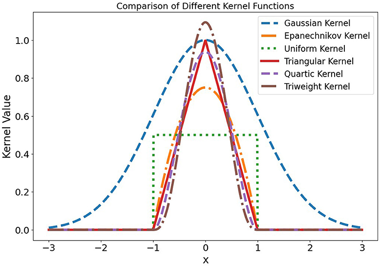
Figure 1. Comparison of different kernel functions, all centered at zero and using a bandwidth of one.

2.2 K-nearest neighbor regression

KNN regression is a type of non-parametric method used for predicting the continuous outcome of a new data point based on the outcomes of its nearest neighbors in the feature space. It does not make any assumptions about the underlying data distribution and is particularly useful when dealing with complex data structures (Hastie et al., 2009). Given a dataset with n points, (x₁, y₁), (x₂, y₂), ..., (x_n, y_n), where each x_i represents a vector of features and each y_i represents the corresponding continuous outcome, KNN regression predicts the outcome ŷ for a new data point x based on the outcomes of its k nearest neighbors in the feature space. The mathematical formulation of KNN regression includes (Altman, 1992):

• Distance metric: the first step in KNN regression is to determine the “closeness” of data points in the feature space, which requires a distance metric. The most common choice is the Euclidean distance, though other metrics like Manhattan or Minkowski can also be used. The distance d between two data points x and x_i is calculated by using Equation (7) for Euclidean distance.

$\begin{array}{ll}d(x,x_i)=\sqrt{{(x-x_i)}^T(x-x_i)}& (7)\end{array}$

• Finding neighbors: for a given data point x, find the k points in the dataset that are closest to x based on the distance metric. These points are termed KNN.

• Prediction: The predicted outcome ŷ is calculated as the average of the outcomes of the k-nearest neighbors. Mathematically, this can be represented as:

$\begin{array}{ll}ŷ=\frac{1}{k}{\sum }_{i\in N_k}{y}_i.& (8)\end{array}$

• In Equation (8), N_k contains the indices of the k closest (in l₂ distance) of x₁, ..., x_n to x.

Figure 2 illustrates the example of the KNN regression with k = 10, where the dataset was synthetically generated from model Y = sin(x)+ sin(2x)+ε. It can be observed that KNN regression makes no assumptions about linearity and fits the data well. The predictions for new data points are based on the average outcomes of the 9 nearest points from the training data.

Figure 2

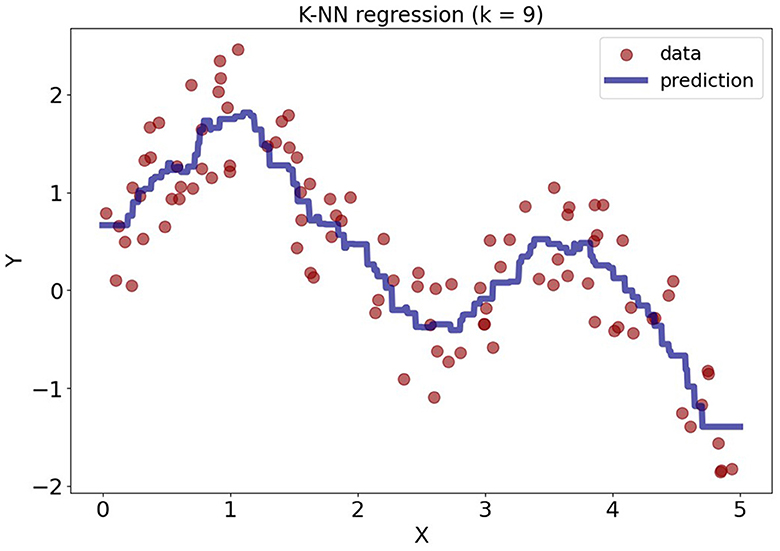
Figure 2. KNN regression model with k = 9 applied to synthetically generated data.

2.3 Kernel k-nearest neighbor regression

Kernel k-Nearest Neighbor (K-KNN) regression extends the conventional KNN regression algorithm, an instance-based learning method, by incorporating kernel functions. This integration allows the algorithm to weigh the contributions of each point's neighbors based on their distance, effectively smoothing out predictions and improving the model's ability to handle complex, non-linear relationships (Tan et al., 2020; Yao et al., 2021). Given a dataset with n points (x₁, y₁), (x₂, y₂), ..., (x_n, y_n), where each x_i represents a vector of features and each y_i represents the corresponding continuous outcome, the prediction ŷ for a new data point x is calculated not just by averaging the outcomes of its k but by taking a weighted average, where the weights are determined by a kernel function based on the distance between x and each x_i.

The kernel function K in Equation (9) applied in this context is a symmetric function that satisfies certain mathematical conditions (like positivity and integrability) with the general form K:ℝ^d → ℝ, where d is the dimension of the input space. The kernel function K must satisfy

$\begin{array}{ll}\int K(t)dt=1,\int tK(t)dt=0,0<\int t^{2}K(t)dt<\infty .& (9)\end{array}$

The choice of kernel function can significantly influence the regression outcome, as different kernels impose different structures on the data (Hofmann et al., 2008). The prediction ŷ in K-KNN regression is then given by:

$\begin{array}{ll}ŷ=\frac{\sum _{i\in N_k}K(x,x_i)·y_i}{\sum _{i\in N_k}K(x,x_i)}.& (10)\end{array}$

In Equation (10) K(x, x_i) is the kernel function evaluating the similarity (or smoothness) between the target point x and each neighbor x_i.

2.4 Cross-validation for optimal parameters

It is imperative to determine the optimal k for the neighbors and the best-suited bandwidth for the kernel function in the context of each bootstrap sample. This step ensures that the model is not just fitted to the training data but also generalizes well to unseen data.

Utilizing ν−fold cross-validation, the original training set is randomly partitioned into ν equal-sized subsamples. Of the ν subsamples, a single subsample is retained as the validation data for testing the model, and the remaining ν−1 subsamples are used as training data. The cross-validation process is then repeated ν times (the folds), with each of the ν subsamples used exactly once as the validation data. For each fold and each candidate combination of parameters (specific k and bandwidth), the model is trained, and the prediction error (e.g., RMSE) on the validation fold is computed. The average error across all ν folds is then calculated for each combination (Wong and Yang, 2017; Wong and Yeh, 2020).

3 Proposed method

Combining bootstrap sampling, choosing features at random, and using kernel methods in a KNN model is employed to make standard KNN better at prediction. Given a training dataset LD(X; Y), where X is a p-dimensional feature matrix with n observations and Y is the corresponding response variable, the objective is to predict the response ŷ for a new observation x₀ in the test dataset. Note that in KNN regression, it is essential to preprocess all predictors to ensure they are unitless. The step for random kernel KNN (RK-KNN) regression is as follows:

1) Bootstrap Sampling for KNN

Bootstrap sampling is integral to ensemble methodologies, particularly bagging. It involves generating B unique datasets from the original training data, D, each termed D_b (where b = 1, 2, …, B) by sampling n observations with replacement. In mathematical notation,

$\begin{array}{ll}{D}_b=\left\{(x_1^{{}^{*}},y_1^{{}^{*}}),(x_2^{{}^{*}},y_2^{{}^{*}}),\dots ,(x_n^{{}^{*}},y_n^{{}^{*}})\right\}.& (11)\end{array}$

In this study, B is set to 1,000.

3) Random Feature Selection

Incorporating a feature randomness aspect akin to Random Forests, each bootstrap sample D_b, as shown in Equation (11), undergoes a feature selection process where only a random subset of d features (where d<p) is considered for model training. During the training phase for each D_b, the algorithm does not utilize the full feature set. Instead, it randomly selects a subset, contributing to model diversity within the ensemble (Breiman, 2001). In this study, d is set to p/2, p/5, and $\sqrt{p}$, and the best d is determined from one that yields the lowest RMSE or MAE or highest R².

3) Kernel Enhancement in KNN

We add the Gaussian, Epanechnikov, uniform, triangular, quartic, and tricube kernels to a standard KNN in this paper. Within KNN, kernel functions can adjust neighbor contributions, giving more weight to nearer neighbors. Suppose N_k(x₀) denotes the set of k nearest neighbors to a query point x₀, determined using a subset of d features. The kernel-weighted response estimate is given by:

$\begin{array}{ll}ŷ=\frac{\sum _{x_i\in N_k(x_0)}K(x_0,x_i)·y_i}{\sum _{x_i\in N_k(x_0)}K(x_0,x_i)}.& (12)\end{array}$

In Equation (12), K(x₀, x_i) is the kernel function evaluating the closeness of points x₀ and x_i, and y_i are the response values of the neighbors. Note that all x_i are needed to be rescaled to be in [0, 1]. This scaling not only helps remove unit dominance but also easily helps determine the bandwidth value of the kernel functions.

4) Determining Optimal k and Bandwidth

The optimal k and bandwidth parameters are those that minimize the average prediction error estimated through a 5-fold cross-validation. Let's denote the set of candidate k values as {k₁, k₂, ..., k_r} and the set of candidate bandwidths as {h₁, h₂, ..., h_s}. The objective is to find the optimal k_opt and h_opt that yield the lowest estimated prediction error:

$\begin{array}{ll}(k_{opt},h_{opt})=arg{\displaystyle \underset{k_i,h_j}{min}}CV(k_i,h_j).& (13)\end{array}$

In Equation (13), CV(k_i, h_j) represents the cross-validation error estimated over multiple random splits of the dataset into training and validation sets. Because all variables are scaled between 0 and 1, the distance between any two points will also fall within a bounded interval. This boundedness allows for the selection of h based on the maximum distance within the k-nearest neighbors for each query point, specifically for k = 2, 3, 5, 7. This method ensures that h is sufficiently large to encompass all neighbors in the calculation, thus being responsive to the local structure of the data and accommodating areas of varying density. The optimal (k_opt, h_opt) is found from the grid {k₁, k₂, ..., k_r} × {h₁, h₂, ..., h_s}.

5) Ensemble Prediction

The ensemble's predictive power is harnessed by aggregating the individual KNN models' outputs. If each model provides a prediction ŷ_b for x₀. The final prediction is an aggregate statistic (e.g., mean) of these predictions, as shown in Equation (14):

$\begin{array}{ll}{ŷ}_{final}=\frac{1}{B}{\sum }_{b=1}^B{ŷ}_b.& (14)\end{array}$

The pseudocode below (Algorithm 1) concretizes the sequence of steps—from bootstrap sampling to the ensemble prediction—that collectively forge our proposed method.

Algorithm 1

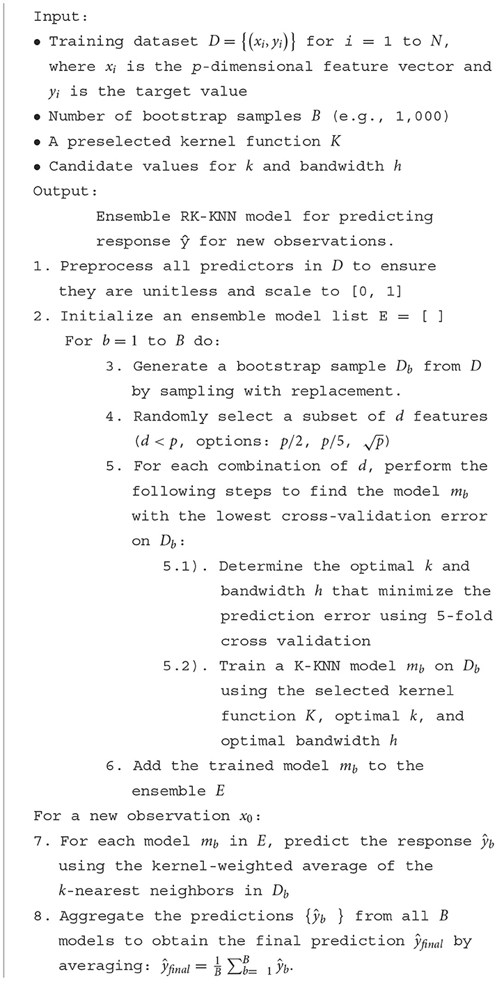
Algorithm 1. RK-KNN model for predicting responses.

4 Evaluation datasets and results

This section is dedicated to presenting the datasets used for benchmarking and the outcomes of the empirical evaluation conducted to assess the effectiveness of the RK-KNN regression approach. Additionally, state-of-the-art methods, including RF, ANN, and SVR, will be compared with the RK-KNN models.

4.1 Datasets for benchmarking

For assessing the new approach alongside existing leading techniques, we utilize 15 distinct datasets. These collections of data are acquired from multiple publicly accessible platforms. An overview of each dataset is presented in Table 1, detailing the number of observations (n), the number of predictor variables (p), and the meaning of the response variable.

Table 1

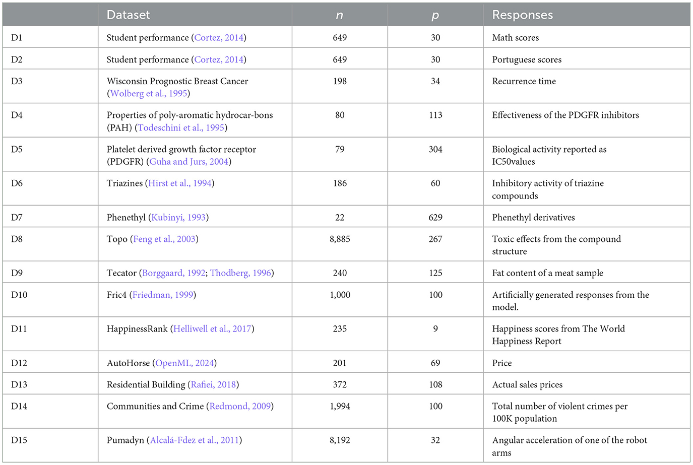
Table 1. Datasets employed for model evaluation in RK-KNN regression with different kernels.

4.2 Performance evaluation

The performance of the RK-KNN method, when compared to the standard KNN and R-KNN, across datasets D1 to D15, is summarized in Table 2. It reveals the effectiveness of the RK-KNN method in enhancing predictive accuracy. The RK-KNN method, particularly when employing specific kernels, consistently outperforms the standard KNN in terms of root mean square serror (RMSE), mean absolute error (MAE), and R-squared (R²) values.

Table 2

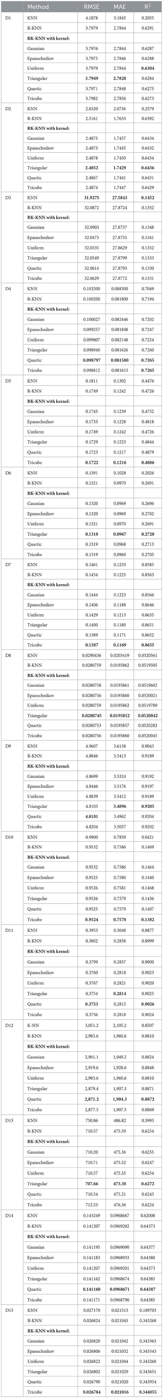
Table 2. Performance evaluation of KNN, R-KNN, and RK-KNN with various kernel functions across datasets (bold values represent the best performance).

Overall, the triangular kernel emerges as the most effective, closely followed by the Tricube kernel. This observation is supported by instances across multiple datasets; for example, in dataset D1, the triangular kernel achieves an RMSE of 3.7949, an MAE of 2.7828, and an R² of 0.6304, surpassing the performance of classical KNN. Similarly, in dataset D6, the triangular kernel demonstrates superior results with an RMSE of 0.1318, an MAE of 0.0967, and an R² of 0.272.

The Gaussian and Epanechnikov kernels tend to not give the lowest RMSE or MAE but still perform notably well compared to the traditional KNN and R-KNN. The uniform kernel sometimes shows superiority compared to the other kernel functions.

Rankings are assigned to the methods from one to eight based on the values of RMSE, MAE, and R². The lowest RMSE or MAE values receive a rank of one, indicating the best performance, while for R², the highest value is awarded a rank of one. The rankings for RMSE, MAE, and R² are summarized in Figures 3–5, respectively. These graphs demonstrate that the RK-KNN regression models generally achieve lower ranks, indicating better performance compared to the R-KNN and traditional KNN regression models. Specifically, for RMSE, the average ranks for RK-KNN with quartic, triangular, tricube, Epanechnikov, Gaussian, and uniform kernels are 1.93, 2.27, 3.13, 3.80, 5.20, and 5.27, respectively. In contrast, the R-KNN and traditional KNN models have average ranks of 6.40 and 7.53, respectively.

Figure 3

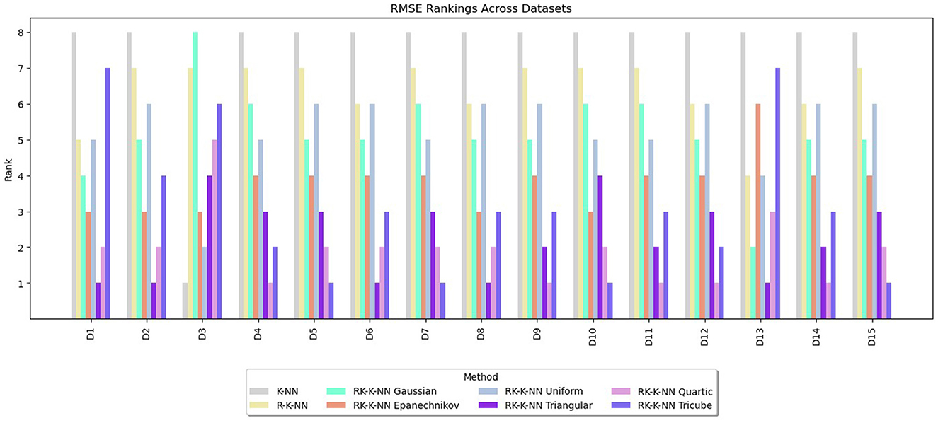
Figure 3. Comparative performance of RK-KNN with different kernel functions, R-KNN, and KNN regressions on multiple datasets using RMSE rankings.

Figure 4

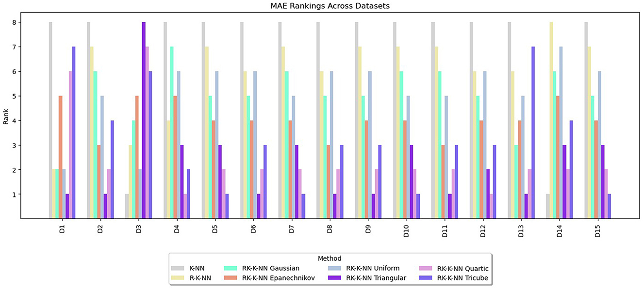
Figure 4. Comparative performance of RK-KNN with different kernel functions, R-KNN, and KNN regressions on multiple datasets using MAE rankings.

Figure 5

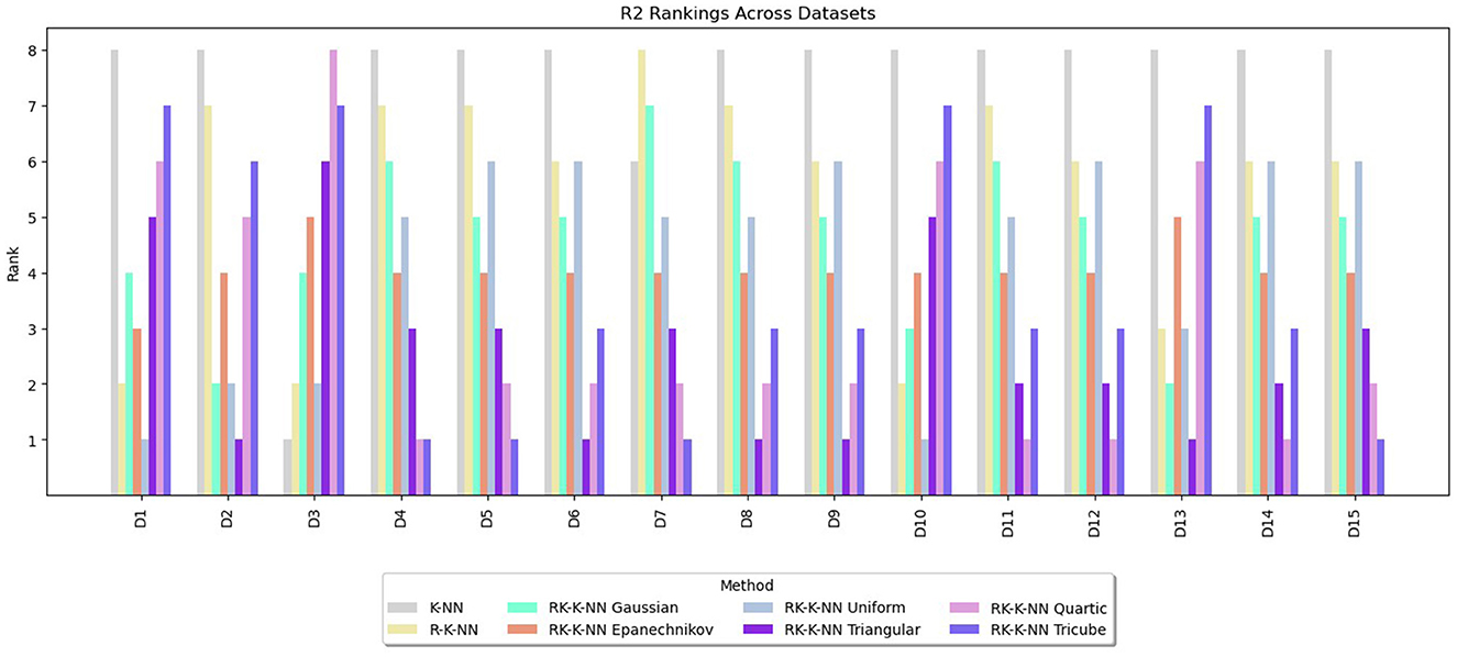
Figure 5. Comparative performance of RK-KNN with different kernel functions, R-KNN, and KNN regressions on multiple datasets using R² rankings.

For MAEs, RK-KNN models with triangular and quartic kernels exhibit nearly identical rankings, with average ranks of 2.33 and 2.67, respectively. The rankings for other methods are consistent with those observed for RMSE. The sequence features RK-KNN with tricube, Epanechnikov, Gaussian, and uniform kernels, followed by R-KNN and KNN, with respective average ranks of 3.27, 4.07, 5.07, 5.20, 6.00, and 7.07.

For R², the RK-KNN model using the triangular kernel shows the best performance, achieving the lowest average rank of 2.60. It is followed by the RK-KNN models with quartic, tricube, Epanechnikov, uniform, and Gaussian kernels. R-KNN and KNN lag behind, with average ranks for R² being 3.13, 3.73, 4.07, 4.33, 4.67, 5.47, and 7.40, respectively.

4.3 Comparisons with state-of-the-art methods

The KNN models exhibiting the lowest RMSEs were benchmarked against RF, ANN, and SVR across fifteen diverse datasets, as detailed in Table 3. KNN-typed learners showed superior performance in datasets D3, D4, D5, D7, and D8, representing a third of the datasets. However, they were notably outperformed by RF in nine datasets (D1, D2, D6, D9, D10, D12, D13, D14, and D15) and by ANN and SVR in the remaining datasets. Although RK-KNN regression did not achieve the lowest RMSE in all datasets, it remains a competitive option, particularly against SVR and ANN. This is especially evident in datasets D5 and D8, which contain a high number of features, where RK-KNN was preferred over the other models.

Table 3

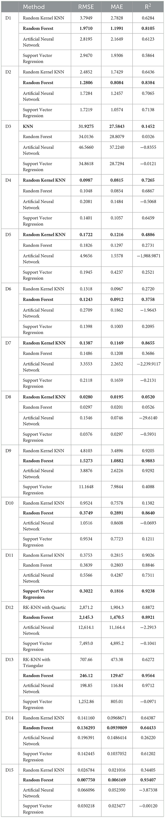
Table 3. Performance evaluation of best KNN-typed learner, RF, ANN, and SVR (bold values represent the best performance).

5 Conclusion and discussion

This study validates the efficacy of integrating kernel functions with a random process, which includes both bootstrapping and feature selection, across 15 datasets. Our comprehensive evaluation, based on criteria such as RMSE, MAE, and R², underscores the superiority of the RK-KNN approach, especially when employing quartic, triangular, and tricube kernel functions. These kernels have consistently demonstrated performance enhancements across various case studies.

Specifically, in dataset D10, RK-KNN regression markedly improves prediction accuracy. The RMSE distributions depicted in Figure 6 reveal that standard KNN exhibits higher RMSE compared to other methods, with all parameter configurations for RK-KNN outperforming standard KNN. However, achieving optimal performance across datasets may require a comprehensive search to identify the best parameters for the selected kernel functions. As shown in Figure 7, while the lowest RMSE values for RK-KNN across all kernel functions are superior to those of KNN, the medians of RMSEs for some kernels, like the Gaussian kernel, exceed the median RMSE of KNN. This variability indicates a critical need for tuning the optimal bandwidth and k-value to consistently achieve the lowest RMSE.

Figure 6

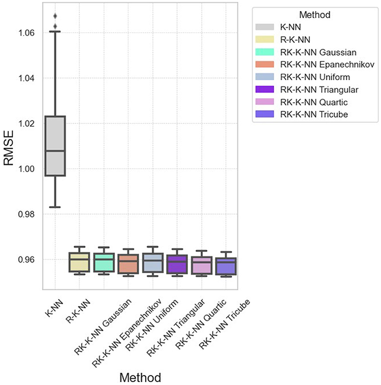
Figure 6. The RMSE distribution across all eight methods for dataset D10.

Figure 7

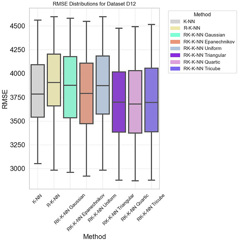
Figure 7. The RMSE distribution across all eight methods for dataset D12.

Moreover, the computational cost and scalability of the RK-KNN algorithm's cross-validation process are effectively managed through vectorized distance computations, which enhance calculation speed and reduce runtime. Standardization of features further contributes to this efficiency by simplifying the distance metric computation. A well-controlled grid search for parameter tuning, along with the ability to independently execute bootstrapping and feature selection steps, ensures computational tractability. Practical applications across multiple datasets have demonstrated that the cross-validation step, a critical aspect of the RK-KNN algorithm, is not prohibitively time-consuming. Therefore, the RK-KNN method is computationally efficient and well-suited for the analysis of large-scale data environments.

Data availability statement

The original contributions presented in the study are included in the article/supplementary material, further inquiries can be directed to the corresponding author.

Author contributions

PS: Conceptualization, Funding acquisition, Investigation, Methodology, Project administration, Writing – original draft, Writing – review & editing. KS: Data curation, Formal analysis, Resources, Software, Visualization, Writing – review & editing.

Funding

The author(s) declare that no financial support was received for the research, authorship, and/or publication of this article.

Acknowledgments

The authors would like to thank the reviewers for their valuable comments and suggestions.

Conflict of interest

The authors declare that the research was conducted in the absence of any commercial or financial relationships that could be construed as a potential conflict of interest.

Publisher's note

All claims expressed in this article are solely those of the authors and do not necessarily represent those of their affiliated organizations, or those of the publisher, the editors and the reviewers. Any product that may be evaluated in this article, or claim that may be made by its manufacturer, is not guaranteed or endorsed by the publisher.

References

Abdalla, H. I., and Amer, A. A. (2022). “Towards highly-efficient k-nearest neighbor algorithm for big data classification,” in 2022 5th International Conference on Networking, Information Systems and Security (New York City, NY: IEEE), 1–5.

Google Scholar

Alcalá-Fdez, J., Fernandez, A., Luengo, J., Derrac, J., García, S., Sánchez, L., et al. (2011). KEEL data-mining software tool: data set repository, integration of algorithms and experimental analysis framework. J. Mult.-Valued Log. Soft Comput. 17, 255–287.

Google Scholar

Ali, A., Hamraz, M., Kumam, P., Khan, D. M., Khalil, U., Sulaiman, M., et al. (2020). A k-nearest neighbours based ensemble via optimal model selection for regression. IEEE Access 8, 132095–132105. doi: 10.1109/ACCESS.2020.3010099

Crossref Full Text | Google Scholar

Altman, N. S. (1992). An introduction to kernel and nearest-neighbor nonparametric regression. Am. Stat. 46, 175–185. doi: 10.1080/00031305.1992.10475879

Crossref Full Text | Google Scholar

Bay, S. D. (1999). Nearest neighbor classification from multiple feature subsets. Intell. Data Anal. 3, 191–209. doi: 10.3233/IDA-1999-3304

Crossref Full Text | Google Scholar

Beitollahi, H., Sharif, D. M., and Fazeli, M. (2022). Application layer DDoS attack detection using cuckoo search algorithm-trained radial basis function. IEEE Access 10, 63844–63854. doi: 10.1109/ACCESS.2022.3182818

Crossref Full Text | Google Scholar

Bermejo, S., and Cabestany, J. (2000). Adaptive soft k-nearest-neighbour classifiers. Pattern Recogn. 33, 1999–2005. doi: 10.1016/S0031-3203(99)00186-7

PubMed Abstract | Crossref Full Text | Google Scholar

Bian, C., and Huang, G. Q. (2024). Air pollution concentration fuzzy evaluation based on evidence theory and the K-nearest neighbor algorithm. Front. Environ. Sci. 12:1243962. doi: 10.3389/fenvs.2024.1243962

Crossref Full Text | Google Scholar

Borggaard C. and Thodberg, H. H.. (1992). Optimal minimal neural interpretation of spectra. Anal. Chem. 64, 545–551. doi: 10.1021/ac00029a018

Crossref Full Text | Google Scholar

Breiman, L. (2001). Random forests. Mach. Learn. 45, 5–32. doi: 10.1023/A:1010933404324

Crossref Full Text | Google Scholar

Cheng, D., Zhang, S., Deng, Z., Zhu, Y., and Zong, M. (2014). “kNN algorithm with data-driven k value,” in Advanced Data Mining and Applications Lecture Notes in Computer Science, 8933. Cham: Springer.

Google Scholar

Chung, Y.-W., Khaki, B., Li, T., Chu, C., and Gadh, R. (2019). Ensemble machine learning-based algorithm for electric vehicle user behavior prediction. Appl. Energy 254, 113732. doi: 10.1016/j.apenergy.2019.113732

Crossref Full Text | Google Scholar

Cortez, P. (2014). Student Performance. Boston: UCI Machine Learning Repository.

Google Scholar

Deng, Z., Zhu, X., Cheng, D., and Zong, M. Zhang, S. (2016). Efficient kNN classification algorithm for big data. Neurocomputing 195, 143–148. doi: 10.1016/j.neucom.2015.08.112

Crossref Full Text | Google Scholar

Dimopoulos, A. C., Nikolaidou, M., Caballero, F. F., Engchuan, W., Sanchez-Niubo, A., Arndt, H., et al. (2018). Machine learning methodologies versus cardiovascular risk scores, in predicting disease risk. BMC Med Res Methodol. 18:179. doi: 10.1186/s12874-018-0644-1

PubMed Abstract | Crossref Full Text | Google Scholar

El-Kenawy, E.-S. M., Mirjalili, S., Ghoneim, S. M., Eid, M. M., El-Said, M., Khan, Z. S., et al. (2021). Advanced ensemble model for solar radiation forecasting using sine cosine algorithm and Newton's laws. IEEE Access 9, 115750–115765. doi: 10.1109/ACCESS.2021.3106233

Crossref Full Text | Google Scholar

Enriquez, A. R. S., Lima, S. L., and Saavedra, O. R. (2019). “K-NN and mean-shift algorithm applied in fault diagnosis in power transformers by DGA,” in Presented at the 2019 20th International Conference on Intelligent System Application to Power Systems (ISAP) (New Delhi: ISAP), 1-6.

Google Scholar

Feng, J., Lurati, L., Ouyang, H., Robinson, T., Wang, Y., Yuan, S., et al. (2003). Predictive toxicology: benchmarking molecular descriptors and statistical methods. J. Chem. Inf. Comput. Sci. 43, 1463–1470. doi: 10.1021/ci034032s

PubMed Abstract | Crossref Full Text | Google Scholar

Friedman, J. H. (1999). Greedy Function Approximation: A Gradient Boosting Machine. Stanford, CA: Technical Report, Department of Statistics, Stanford University.

Google Scholar

García-Pedrajas, N., and Ortiz-Boyer, D. (2009). Boosting k-nearest neighbor classifier by means of input space projection. Expert Syst. Appl. 36, 10570–10582. doi: 10.1016/j.eswa.2009.02.065

Crossref Full Text | Google Scholar

Ghavami, S., Alipour, Z., Naseri, H., Jahanbakhsh, H., and Karimi, M. M. (2023). “A new ensemble prediction method for reclaimed asphalt pavement (RAP) mixtures containing different constituents. Buildings 13:1787. doi: 10.3390/buildings13071787

Crossref Full Text | Google Scholar

Guha, R., and Jurs, P. C. (2004). Development of linear, ensemble, and nonlinear models for the prediction and interpretation of the biological activity of a set of PDGFR inhibitors. J. Chem. Inf. Comput. Sci. 44, 2179–2189. doi: 10.1021/ci049849f

PubMed Abstract | Crossref Full Text | Google Scholar

Hastie, T., Tibshirani, R., and Friedman, J. (2009). The Elements of Statistical Learning: Data Mining, Inference, and Prediction. Springer Series in Statistics, 2nd ed. (New York, NY, USA: Springer).

Google Scholar

Helliwell, J., Layard, R., and Sachs, J. (2017). World Happiness Report 2017. New York: Sustainable Development Solutions Network. Available online at: https://worldhappiness.report/ed/2017/ (accessed January 9, 2024).

Google Scholar

Hirst, J. D., King, R. D., and Sternberg, M. J. (1994). Quantitative structure-activity relationships by neural networks and inductive logic programming. II. The inhibition of dihydrofolate reductase by triazines. J. Comput. Aided Mol. Des. 8, 421–432. doi: 10.1007/BF00125376

PubMed Abstract | Crossref Full Text | Google Scholar

Hofmann, T., Schölkopf, B., and Smola, A. J. (2008). Kernel methods in machine learning. Ann. Statist. 36, 1171–1220. doi: 10.1214/009053607000000677

Crossref Full Text | Google Scholar

Ingram, S., and Munzner, T. (2015). Dimensionality reduction for documents with nearest neighbor queries. Neurocomputing 150, 557–569. doi: 10.1016/j.neucom.2014.07.073

PubMed Abstract | Crossref Full Text | Google Scholar

Jafar, R., Awad, A., Hatem, I., Jafar, K., Awad, E., and Shahrour, I. (2023). Multiple linear regression and machine learning for predicting the drinking water quality index in Al-seine lake. Smart Cities 6, 2807–2827. doi: 10.3390/smartcities6050126

Crossref Full Text | Google Scholar

Jiang, Z., Yang, S., Smith, P., and Pang, Q. (2023). Ensemble machine learning for modeling greenhouse gas emissions at different time scales from irrigated paddy fields. Field Crops Res. 292:108821. doi: 10.1016/j.fcr.2023.108821

Crossref Full Text | Google Scholar

Kubinyi, H. (1993). QSAR: Hansch Analysis and Related Approaches. Methods and Principles in Medicinal Chemistry. Weinheim; New York, NY: Wiley-VCH, 438.

Google Scholar

Li, Q.-c., Xu, S.-w., Zhuang, J.-y., Liu, J.-j., Zhou, Y., and Zhang, Z.-x. (2023). Ensemble learning prediction of soybean yields in China based on meteorological data. J. Integr. Agric. 22, 1909–1927. doi: 10.1016/j.jia.2023.02.011

Crossref Full Text | Google Scholar

Li, S., Harner, E. J., and Adjeroh, D. A. (2014). “Random KNN,” in Presented at the 2014 IEEE International Conference on Data Mining Workshop, Shenzhen, China (Los Alamitos, CA; Washington, DC; Tokyo: IEEE Computer Society Conference Publishing Services (CPS)) 629–636.

Google Scholar

OpenML (2024). dataset-autoHorse_fixed. Available online at: https://www.openml.org/d/42224 (accessed February 02, 2024).

Google Scholar

Pramanik, P. K.D., Mukhopadhyay, M., and Pal, S. (2021). “Big data classification: applications and challenges,” in Artificial Intelligence and IoT. Studies in Big Data, eds. K. G. Manoharan, J. A. Nehru, and S. Balasubramanian (Singapore: Springer).

Google Scholar

Rafiei, M. (2018). Residential Building Data Set. Boston: UCI Machine Learning Repository.

Google Scholar

Redmond, M. (2009). Communities and Crime. Boston: UCI Machine Learning Repository.

Google Scholar

Rubio, G., Guillen, A., Pomares, H., Rojas, I., Paechter, B., Glosekotter, P., et al. (2009). “Parallelization of the nearest-neighbour search and the cross-validation error evaluation for the kernel weighted k-nn algorithm applied to large data sets in MATLAB,” in Presented at the 2009 International Conference on High Performance Computing & Simulation (New York City, NY: IEEE), 1–6.

Google Scholar

Saadatfar, H., Khosravi, S., Joloudari, J. H., Mosavi, A., and Shamshirband, S. (2020). A new K-nearest neighbors classifier for big data based on efficient data pruning. Mathematics 8:286. doi: 10.3390/math8020286

Crossref Full Text | Google Scholar

Schölkopf, B., and Smola, A. J. (2001). Learning with Kernels: Support Vector Machines, Regularization, Optimization, and Beyond, 1st ed. Cambridge, MA: MIT Press.

Google Scholar

Sharma, S., and Lakshmi, L. R. (2023). “Improved k-NN regression model using random forests for air pollution prediction,” in Presented at the International Conference on Smart Applications, Communications, and Networking (SmartNets) (Istanbul: SmartNets).

Google Scholar

Song, H., and Choi, H. (2023). Forecasting stock market indices using the recurrent neural network based hybrid models: CNN-LSTM, GRU-CNN, and ensemble models. Appl. Sci. 13:4644. doi: 10.3390/app13074644

Crossref Full Text | Google Scholar

Song, J., Zhao, J., Dong, F., Zhao, J., Qian, Z., and Zhang, Q. (2018). A novel regression modeling method for PMSLM structural design optimization using a distance-weighted KNN algorithm. IEEE Trans. Indust. Appl. 54, 4198–4206. doi: 10.1109/TIA.2018.2836953

Crossref Full Text | Google Scholar

Srisuradetchai, P. (2023). A novel interval forecast for k-nearest neighbor time series: a case study of durian export in Thailand. IEEE Access. 12, 2032–2044. doi: 10.1109/ACCESS.2023.3348078

Crossref Full Text | Google Scholar

Srisuradetchai, P., and Panichkitkosolkul, W. (2022). “Using ensemble machine learning methods to forecast particulate matter (PM_2.5) in Bangkok, Thailand,” in Multi-disciplinary Trends in Artificial Intelligence, eds. O. Surinta and K. F. Yuen (Cham: Springer).

Google Scholar

Srisuradetchai, P., Panichkitkosolkul, W., and Phaphan, W. (2023). “Combining machine learning models with ARIMA for COVID-19 epidemic in Thailand,” in Proceedings of the 2023 Research, Invention, and Innovation Congress: Innovation in Electrical and Electronics (RI2C), Bangkok, Thailand (New York City, NY: IEEE), 155–161.

Google Scholar

Steele, B. M. (2009). Exact bootstrap k-nearest neighbor learners. Mach. Learn. 74, 235–255. doi: 10.1007/s10994-008-5096-0

Crossref Full Text | Google Scholar

Tan, R., Ottewill, J. R., and Thornhill, N. F. (2020). Monitoring statistics and tuning of Kernel principal component analysis with radial basis function kernels. IEEE Access 8, 198328–198342. doi: 10.1109/ACCESS.2020.3034550

Crossref Full Text | Google Scholar

Thodberg, H. H. (1996). A review of Bayesian neural networks with an application to near infrared spectroscopy. IEEE Trans. Neural Networks 7, 56–72. doi: 10.1109/72.478392

PubMed Abstract | Crossref Full Text | Google Scholar

Todeschini, R. Gramatica, P., Pravenzani, R., and Marengo, E. (1995). Weighted holistic invariant molecular descriptors. Part 2. Theory development and applications on modeling physicochemical properties of polyaromatic hydrocarbons. Chemometrics Intell. Lab. Syst. 27, 221–229. doi: 10.1016/0169-7439(94)00025-E

Crossref Full Text | Google Scholar

Tsybakov, A. B. (2009). Introduction to Nonparametric Estimation. 1st ed. New York, NY: Springer.

Google Scholar

Ukey, N., Yang, Z., Li, B., Zhang, G., and Hu, Y. Zhang, W. (2023). Survey on exact kNN queries over high-dimensional data space. Sensors 23:629. doi: 10.3390/s23020629

PubMed Abstract | Crossref Full Text | Google Scholar

Wolberg, W., Mangasarian, O., Street, N., and Street, W. (1995). Breast Cancer Wisconsin (Diagnostic). Boston: UCI Machine Learning Repository.

Google Scholar

Wong, T.-T., and Yang, N.-Y. (2017). Dependency analysis of accuracy estimates in k-fold cross validation. IEEE Trans. Knowl. Data Eng. 29, 2417–2427. doi: 10.1109/TKDE.2017.2740926

Crossref Full Text | Google Scholar

Wong, T.-T., and Yeh, P.-Y. (2020). Reliable accuracy estimates from k-fold cross validation. IEEE Trans. Knowl. Data Eng. 32, 1586–1594. doi: 10.1109/TKDE.2019.2912815

Crossref Full Text | Google Scholar

Yao, Y., Li, Y., Jiang, B., and Chen, H. (2021). Multiple kernel k-means clustering by selecting representative kernels. IEEE Trans. Neural Netw. Learn. Syst. 32, 4983–4996. doi: 10.1109/TNNLS.2020.3026532

PubMed Abstract | Crossref Full Text | Google Scholar

Zheng, G., and Cao, G. (2008). “A Modified K-NN algorithm for holter waveform classification based on kernel function,” in 2008 Fifth International Conference on Fuzzy Systems and Knowledge Discovery, Jinan, China (Los Alamitos, CA; Washington, DC; Tokyo: IEEE Computer Society Conference Publishing Services (CPS)), 343–346.

Google Scholar