
94% of researchers rate our articles as excellent or good
Learn more about the work of our research integrity team to safeguard the quality of each article we publish.
Find out more
ORIGINAL RESEARCH article
Front. Big Data, 18 December 2020
Sec. Medicine and Public Health
Volume 3 - 2020 | https://doi.org/10.3389/fdata.2020.572134
This article is part of the Research TopicML and AI Safety, Effectiveness and Explainability in HealthcareView all 5 articles
 Gerald P. Clarke1*
 Adam Kapelner2*
Purpose: Our work introduces a highly accurate, safe, and sufficiently explicable machine-learning (artificial intelligence) model of intraocular lens power (IOL) translating into better post-surgical outcomes for patients with cataracts. We also demonstrate its improved predictive accuracy over previous formulas.
Methods: We collected retrospective eye measurement data on 5,331 eyes from 3,276 patients across multiple centers who received a lens implantation during cataract surgery. The dependent measure is the post-operative manifest spherical equivalent error from intended and the independent variables are the patient- and eye-specific characteristics. This dataset was split so that one subset was for formula construction and the other for validating our new formula. Data excluded fellow eyes, so as not to confound the prediction with bilateral eyes.
Results: Our formula is three times more precise than reported studies with a median absolute IOL error of 0.204 diopters (D). When converted to absolute predictive refraction errors on the cornea, the median error is 0.137 D which is close to the IOL manufacturer tolerance. These estimates are validated out-of-sample and thus are expected to reflect the future performance of our prediction formula, especially since our data were collected from a wide variety of patients, clinics, and manufacturers.
Conclusion: The increased precision of IOL power calculations has the potential to optimize patient positive refractive outcomes. Our model also provides uncertainty plots that can be used in tandem with the clinician’s expertise and previous formula output, further enhancing the safety.
Translational relavance: Our new machine learning process has the potential to significantly improve patient IOL refractive outcomes safely.
Pre-operative intraocular lens (IOL) power predictions are essential to patient refractive outcomes on implanted lenses in cataract surgery and thus ophthalmologists have been interested in accurate predictions for a long time. Before the introduction of mathematical prediction formulas, IOL power was inferred from patient history using educated guesses. This changed in 1981 with the first known formula, the SRK equation, IOL power = A – 2.5L – 0.9K, where L is the axial length in mm, K is the average keratometry in diopters, and A is a constant dependent on properties of the manufactured lens being implanted. This formula is highly interpretable and explainable but due to its simplicity and inaccuracy (especially on eyes that are not of average axial length), an updated formula, the SRK II published in 1989, added a correction for longer- and shorter-than-average axial length eyes, allowing predictions for a greater proportion of the population. Further accuracy was obtained in the SRK/T formula in 1990 which added corrections based on anterior chamber depth.
The trend has continued where each new generation of formula provides higher accuracy by (1) incorporating new measurements on the patient’s eye and (2) employing more complex mathematical expressions to model the relationship. Substantial improvements have only occurred in the last 15 years where (1) we now collect more ocular biometry measurements with greater precision and (2) we use more advanced modeling due to advances in computing power and artificial intelligence algorithms. For (1) we now have many non-traditional IOL biometry variables, such as anterior chamber depth (ACD, also known as “epithelium to anterior lens”), corneal diameter, and corneal shape all feature complex unknown relationships with IOL power that are difficult to model with traditional regression and Gaussian optics (Holladay et al., 1988; Hoffer, 1993; Haigis et al., 2000). For (2), Clarke and Burmeister, (1997) first proposed using neural networks to predict lens powers. This led to a significant increase in predictive accuracy, even before the advent of modern optical biometry. Recently, Hill et al. designed a radial basis function neural net that extracts features and relationships from a large dataset to predict the optimal emmetropic IOL power (hence forward termed “RBF 1.0 calculator”). This computational process is available on the ASCRS website and commercially at RBFcalculator.com. For the state of the art, standard deviation of prediction error in refraction is between 0.361 and 0.433 (Cooke and Cooke, 2016).
Herein, we present a more advanced formula that not only improves prediction accuracy, but offers additional practical advantages. Our contribution can be summarized by four points.
First, we begin with a large training dataset compiled from several surgeons over approximately three years of implanting many different IOLs (see Table 1 for a list of lenses). We then collected more information about each patient than has been considered in previous research, i.e., advancing accuracy via (1).
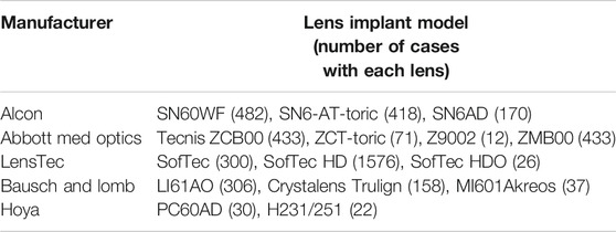
TABLE 1. Manufacturers and lenses used in our dataset with the number of cases with each lens. Some of these cases were excluded from the study due to insufficient post-op data, less than 20/30 post-op best-corrected vision, and other reasons.
Second, our formula is machine-learned using the state-of-the-art algorithm that sums decision trees. This model called “Bayesian Additive Regression Trees” (BART), an out-of-the-box predictive modeling algorithm that is known for high predictability (Chipman et al., 2010; Kapelner and Bleich, 2016). BART has several advantages over other computational algorithms: it allows for highly accurate fitting of non-linear relationships of the patient measurements and interaction of these measurements to our predictive target, i.e., improving accuracy via (2). Additionally, BART allows for measurement “missingness” to be incorporated naturally without the need for imputation. Also, BART uses Monte Carlo simulations to gauge its own accuracy and outputs an interval of possible lens powers with a probability density.
Third, note that previous formulas predicted Effective Lens Position (ELP) and then converted it to IOL power post facto. This conversion can introduce another source of error. Thus, we further improve accuracy in (2) by predicting IOL power directly, obviating the need for the post facto correction.
Fourth, we use BART to predict the difference between the back-calculated ideal implanted lens power and the standard SRK/T calculation for lens power for the obtained refraction AL-adjusted. This follows the approaches of Wang et al., (2011) and Savini et al., (2015) who adjust the standard formulas for long AL and corneal shape. We employ the AL adjustment of the former herein. Thus, our statistical modeling intention is to correct the error between the SRK/T theoretical-axial length (AL) adjusted lens power calculation and what we observe post-operation. This strategy to leverage the known physics allows us to further improve accuracy via (2).
The result of these four improvements lead to an overall estimate of median absolute lens power error of 0.204 D for future patients. This is of the same order as IOL manufacturer error tolerance (Savini et al., 2015) which we believe is the highest accuracy to date. We also believe our approach provides the highest applicability to non-standard patient profiles to date.
Is there a downside in safety when using our advanced formula? Sometimes yes and sometimes no. Our justification for why the answer is “no” when using our formula can be found in the discussion Our Formula’s Safety. Before doing so, we must discuss our data, our formula, validating its accuracy, comparison to other formulas as well as additional features of our approach and use cases.
A total of 5,331 eyes from 3,276 patients implanted between October 2013 and June 2016 were initially entered for analysis. Patient data (pre-op and post-op) were retrieved anonymously from 13 surgical practices who entered data into a HIPAA compliant secure, encrypted website (www.fullmonteiol.com) developed by Clarke.
Eyes were included if they had uneventful in-the-bag placement of any of several lenses from the manufacturers listed in Table 1. Eyes were excluded if pre-operative variables exceeded the allowed ranges of the RBF 1.0 calculator. Additionally, eyes with ocular pathology and pre-operative corneal (refractive) surgery were excluded. Patients with best corrected post-op vision worse than 20/30 were excluded. Post-operative refractions were not cycloplegic, performed by technicians or optometrists in the retrospective surgical practices. Length of refractive lane was not known. Refractive vertex was assumed to be 12 mm as standard. We ensured that if a patient had surgery on both eyes, then only one of the two eyes at random would belong to the dataset. This was to prevent possible overly optimistic models due to “both eyes bias”.
This study conformed to ethics codes based on the tenets of the Declaration of Helsinki and as the data are de-identified retrospective data; thus our study is exempt from IRB review under 45 CFR 46.104(d)(2) by any of the three options (1), (2), or (3).
We tried to collect many different types of measurements and features. First, all patients were measured pre-operatively with either the Lenstar LS 900 or the IOL Master (versions 3.02 and 5.4, respectively). All surgeons recorded the eye (OD/OS), measured flat keratometry and steep keratometry at 2 mm, 3 mm, and 5 mm, anterior chamber depth (ACD – endothelium to anterior lens), and axial length (AL). Biometry supplied corneal radii, flat and steep, with steep axis, central cornel thickness, retinal thickness, refractive sphere, cylinder, axis, and capsulorhexis. Surgeons also supplied pre-operative target refraction, patient age, whether there was post-refractive surgery, and the lens implant model. Recording the implant model was important as we found there are lens-to-lens idiosyncrasies that affect IOL power (see Explainability: Variable Importance on the variable importance section).
Other variables were supplied on a surgeon-by-surgeon basis. Several surgeons used the LenStar OLCR biometer, which measures central corneal thickness and lens thickness in addition to other variables. Surgeons using Zeiss IOL Master measured corneal diameter (formerly known as “white-to-white”). In addition, Clarke and one of the data contributors (Zudans), measured an ultrasonic biometry variable similar to the external corneal diameter, but measured this internally as sulcus-to-sulcus diameter (857 or 16% cases), and then perpendicular from this line to the corneal epithelial apex, the sulcus-to-sulcus depth similar to the anterior chamber depth (details available on request). Clarke also routinely measured corneal shape as the keratometric Q-factor, recently reported by Savini et al., (2015) to be significant. The total count of patient- and eye-specific characteristics comes to 29. Under no circumstances were post-op measurements included.
We augment these physical measurements by computing 15 theoretical variables from the pre-op measurements. First of these are the optimized SRK/T A-Constant, Holladay Surgeon Factor, Hoffer ACD, and the three Haigis constants, which were calculated for each lens and surgeon using the Haigis linear regression (Haigis et al., 2000). However, many lenses and surgeons did not have enough data to calculate all Haigis constants, hence the Haigis formula performed poorly when separately computed. These subjects’ Haigis constants were then considered missing. The A-Constant, Holladay SF, and Hoffer ACD optimization were calculated with regression for each surgeon/lens to yield emmetropia on average for the respective formulas. Other calculated variables included the SRK/T IOL, Wang-Koch Adjusted (Wang et al., 2011), SRK/T calculated expected refraction, SRK/T ELP, Haigis ELP and IOL, and Holladay calculated ELP and the Holladay IOL power, and the Hoffer ELP and IOL power (Holladay et al., 1988).
In total, we have 44 possible variables per eye (29 physical measurements plus 15 theoretical metrics) denoted x1, x2, …, x44. Each patient’s refraction and implanted IOL power was recorded post-op after a minimum of six weeks (denoted yIOL). Modern machine learning techniques can construct formulas from large input datasets with many variables and we turn to this now.
The data, consisting of 3,276 eyes (all fellow eyes were dropped at random from the 5,331 eye surgeries) were loaded into a data frame in R Core Team, (2018). Before we began to fit a model, we acknowledged that data-driven methods making use of a vast number of patient characteristics (as in our situation) have a tendency to “over-fit” the data and thus give an unrealistically optimistic estimate of future predictive accuracy (Hastie and Tibshirani, 2001). Thus, before beginning any modeling, we split the 3,276 eyes randomly into two sets: a training data set of 80% (2,621 eyes) and a test data set of 20% (655 eyes). The test data are set aside and used for validation which will be addressed in the next section.
We define our prediction target (the dependent variable denoted y) as the difference between the true implanted IOL and the theoretical (AL adjusted) SRK/T IOL power that gives the same post-operative refraction (i.e., y = yIOL - ySRK/T). Thus, our statistical modeling intention is to correct the error between the SRK/T theoretical lens power calculation and what we observe post-operation; this leverages the prediction potential of the optical model of the eye. Our procedure thus refines our knowledge of optics by correcting its systematic errors.
To create our formula, we must accurately fit the functional relationship (denoted f) in the model y = f (x1, x2, …, x44) + ε where ε is considered a catch-all for irreducible noise such as relevant patient characteristics we failed to assess (unknown unknowns) and pre- and post-operative measurement error. To fit the relationship f, we make no assumptions on its structure (e.g., linearity or additivity) and thus we wish to employ a non-parametric statistical learning procedure, i.e., the hallmark of “machine learning.” Note that this is the modeling philosophy also taken by the RBF 1.0 calculator who employ the machine learning method called “kernel regression.”
Here we use the algorithm Bayesian Additive Regression Trees (BART) to create our formula (synonymously refered to as our “BART model”). BART is the sum of a binary decision trees model. Decision trees are sets of rules that look like “if AL < 24, follow the rule on left, otherwise the rule on the right.” If the rule does not point to another nested rule, it will reveal a predicted value. Summing trees together provides higher accuracy since the resultant model is less coarse in its fit of a high-dimensional space such as our 44-variable space. Each crevice of the 44-dimensional space defined by the many trees’ binary rules has IOL powers that are considered Gaussian-distributed, an idea that goes back to Laplace in the late 1700s and is the standard assumption in statistical modeling (e.g., linear regression). The rules and predicted values are considered parameters in a statistical model and these parameters are then estimated with our data from Data Collection and Inclusion Criteria. Further, since BART’s perspective is Bayesian, our model can provide confidence of its estimates from its parameters’ posterior distributions (Chipman et al., 2010).
To fit a BART model to our data, we use the R package bartMachine (Kapelner and Bleich, 2016) which includes native missingness handling (Kapelner and Bleich, 2015). We define “missingness” as an attempt to both fit a model on eyes and/or predict on eyes where not all the 29 patient-specific measurements and/or the 15 theoretical pre-op variables are available. “Native missingness handling” means the algorithm allows for (1) constructing models from data that contains missingness and (2) predicting IOL power for patients’ eyes where not all variables were measured. The algorithm does both without the need for a preliminary imputation step, i.e., providing guesses for the missing patient- and eye-specific measurements. Feature (1) is especially advantageous because a model built with a certain subset of the eye measurements may be very different than a model with a different subset of the data. BART combines these multiple models together automatically. Figure 1 shows a schematic of our model fitting and prediction procedure.
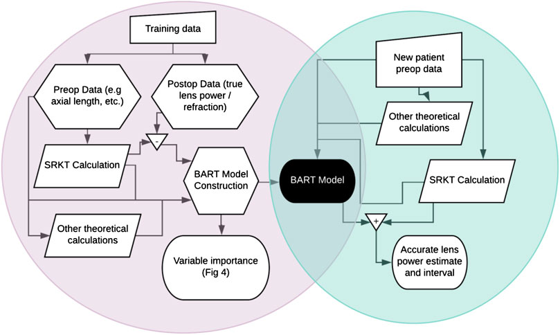
FIGURE 1. Flowchart of (A) BART model creation in the left circle and (B) patient lens power prediction in the right circle. Training data enables the creation of a Bayesian Additive Regression Trees (BART) model which can then be used to predict lens power for future patients.
It is important to stress that non-parametric function estimation has a great practical disadvantage. Although we can predict very accurately, it is atheoretical; we do not know exactly how the patient measurements are combined to produce an IOL power estimate (Breiman, 2001). These methods are often referred to as “black box” methods, as the inner mechanics are not apparent and the assessment of the statistical significance level of a variable’s contribution (as in a linear regression) is elusive.
Even though they are more accurate, these black box methods such as BART do not produce a model fit that corresponds to the “true” function f in any absolute sense. As famously stated by Box and Draper, “all models are wrong, but some are useful” (Box and Draper, 2001). Our model is quite accurate and thereby useful for helping surgeons improve their patients’ outcomes even though in an absolute sense it is not a true physical model nor do we know precisely how it works.
The training data were inputted into the BART algorithm to create a BART model. To validate this BART model, we employ it to predict on the “out-of-sample” test data. These results are an honest estimate of how a practitioner will see our model perform on an arbitrary future patient as our algorithm was blind to the test data.
Since our training data/test data split may have been idiosyncratic, we perform this procedure multiple times using 5-fold cross-validation (Hastie and Tibshirani, 2001). This means that several sets of trials were performed, as follows: 20% of the data were randomly excluded as a test set, and the algorithm was trained over the remaining 80%. This was repeated for five runs, rotating the 20%-sized test set until each eye was out-of-sample once.
We perform this same split-data procedure (model creation on the training data and validation on the test data) for the same specific splits for five comparison models: the RBF 1.0 calculator, the SRK/T formula, Holladay 1 formula, Hoffer-Q formula, and Haigis formula. Note that because the actual test data were not planned emmetropic, the RBF 1.0 calculator’s emmetropic IOL power was adjusted using Gaussian optics to yield the IOL power that produced the actual post-operative spherical equivalent refraction. The correction used is
where “Ref” is the desired post-op refraction (plano in this conversion), “Vtx” is the vertex distance assumed to be 12 mm, K is the average keratometry, and AL is the axial length as in Holladay et al. (1988). For each of the five comparison formulas, the ELP was calculated as in their published formulas.
To compare results with Cooke and Cooke, (2016) and other studies, the prediction errors (the difference between yIOL and the predictions from the three models) was adjusted to the refraction at the corneal plane using a standard vertex distance of 12 mm, yielding the post-operative prediction error. We compare the models using the test data differences of 1) median absolute error via the Wilcoxon rank test, 2) mean absolute error via the t-test, and 3) differences of variances via Levene’s test for non-normal data. Since the same data splits were used for both our BART formula and five competing strategies, the differences in predictive ability are directly comparable.
The BART model outperformed all five competing formulas. Over the 5-fold cross validation, the overall averages of five error metrics are shown in Table 2.
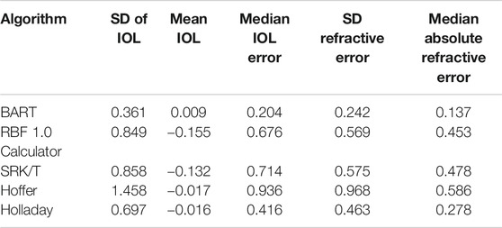
TABLE 2. Results of five random out-of-sample validations with 20% of the data held out.
The overall out-of-sample median absolute IOL error for the BART method was 0.204 D, compared with 0.416 D in Holladay I, 0.676 D in the RBF 1.0 calculator, 0.714 D in the SRK/T formula, 0.936 D for Hoffer-Q, and 1.204 D for Haigis. The standard deviation of the errors for the IOL powers was 0.361 D, 0.463 D, 0.849 D, 0.858 D, 1.458 D, and 1.608 D, respectively. Converting this to the refractive error using Gaussian optics at a vertex of 12 mm yields a standard deviation of 0.242 D (BART), 0.416 D (Holladay I), 0.569 D (RBF 1.0 calculator), 0.575 D (SRK/T), 0.936 D (Hoffer-Q), and 1.48 D (Haigis). The median absolute error (MAE) of refraction were 0.137 D (BART), 0.278 D (Holladay I), 0.45 3D (RBF 1.0 calculator), 0.478 D (SRK/T), 0.586 D (Hoffer-Q), and 1.268 D (Haigis). The Haigis formula performed very poorly in our series probably due to incorrect or missing Haigis constants 1 and 2. Hence, it will not be considered further.
Comparing BART’s absolute error precision to the other five formulas using a one-sample sign test yielded a significant difference (p < 2.2e-16) while there was no significant difference in precision between the RBF 1.0 calculator and SRK/T (p = 0.9). The Holladay 1 calculator was significantly better than the others (p < 0.0004), but still less accurate than the BART MAE. Levene’s tests of the variance for each distribution show BART to be significantly more precise (smaller variance) than all other methods (p < 2.2e-16).
In Figure 2 we plot a regression error curve (Bij et al., 2003) which is a visual performance comparison of BART, the RBF 1.0 calculator, and the SRK/T formula relating cumulative percentages of predictions to levels of absolute prediction error. The plot shows that 95% of the BART predicted IOL power calculations were within approximately ± 0.7 D of the ideal IOL power. This translates with Gaussian optics to 95% of refractions within approximately ± 0.47 D of target refraction. This improvement is seen over the entire range of AL measurements with no systematic error among eyes with short or long AL (see flat trend line in Figure 3). The regression error curve of Figure 2 also shows that 97.4% of BART’s predictions, 87.0% of the RBF 1.0 calculator’s predictions, and 82.9% of the SRK/T formula’s predictions were within ± 1.00 D; 89.5% of BART’s predictions, 61.4% of the RBF 1.0 calculator’s predictions, and 52.0% of the SRK/T formula’s predictions were within ± 0.50 D; and 66.2% of BART’s predictions, 33.4% of the RBF 1.0 calculator predictions, and 27.7% of the SRK/T formula’s predictions were within ± 0.25 D.
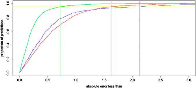
FIGURE 2. A regression error characteristic curve for the absolute error of intraocular lens (IOL) power (in D) for BART (green), the RBF 1.0 calculator (blue), and the SRK/T formula (red) for 1,000 eyes out-of-sample. To interpret this illustration, consider the example of eyes with 0.5 D or less absolute error in their predictions for IOL power. Approximately 90% of BART’s predictions have this level of precision, while approximately 60% of the RBF 1.0 calculator’s predictions and 55% of predictions with the SRK/T formula have such precision. The vertical lines represent the maximum absolute error for 95% of predictions in all three compared approaches.
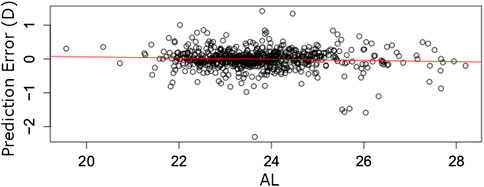
FIGURE 3. Prediction errors (y-axis) for 1,000 eyes out-of-sample arranged by AL (x-axis). The red line fits a linear error trend. The slope of zero implies the BART model’s errors are likely independent of AL.
To compare these result to those of Cooke and Cooke, (2016), we compute the errors in refraction at a vertex of 12 mm. Cooke and Cooke found the standard deviation of post-op refractive prediction error of the highest ranking formula, Olsen (OLCR) on the LenStar machine to be 0.402 D, compared with 0.242 D with our BART method, and median absolute error 0.225 D in post-op refraction, compared to 0.135 D with the BART method. The SRK/T and RBF 1.0 calculator yielded a MAE of refraction of 0.466 D and 0.471 D. The Holladay 1 MAE was 0.278, the second best in our series.
Since our approach is a “black box” formula common in machine learning, a natural question to ask is “how does the formula work?” and further “which measurements were important contributors to our formula”? We discuss explainability in the context of safety and effectiveness in Our Formula’s Safety.
Figure 4 answers the question of “which variables are important?” by plotting the 15 variables with the highest metric of “inclusion proportion”. BART is a model that ultimately looks like a tree which makes binary decisions at the internal nodes (e.g., “AL < 23.84?”). For each internal node in the tree (which could contain hundreds of internal nodes), we tally the variable that defines the decision. In the example of “AL < 23.84?,” we would tally one for the variable AL. The tally of each variable across all nodes defines the proportion of each variables’ inclusion. This inclusion proportion metric is an accepted way to measure degree of variable importance in BART (Kapelner and Bleich, 2016). It can be further used to distinguish statistical significance (that a variable correlates with IOL power) through permutation testing (Bleich et al., 2014) in future work.
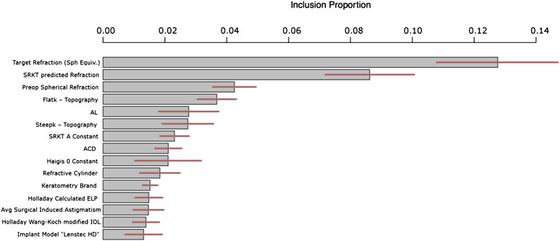
FIGURE 4. Top 15 most important variables for prediction ranked by inclusion proportion in the BART model. The remaining variables have similar inclusion proportions to the least important shown below i.e., approximately 1%. The lines through each bar shows 95% confidence across the BART model’s Monte Carlo simulations.
Figure 4 shows that the most important variable in our predictions that correct the SKR/T formula was intended target refraction. This is not a variable in the classical sense since the clinician specifies it, but nevertheless it is obviously important in the selection of IOL power. The second variable was pre-operative spherical refraction – perhaps this variable encapsulates AL and keratometry. One main observation is that the level of theoretical IOL is absolutely critical to know when correcting the actual IOL error. In other words, the errors in the SRK/T formula are extremely heterogeneous across the gamut of theoretical IOLs. Also, we have features of the SKR/T and Holladay formulas, such as calculated ELP and calculated IOL. We would like to make note of the 15th most important, the “Lenstec HD” implantation. This means this specific implant has its own fitted “submodel” within our overall model. This is likely due to this specific implantation being different than the others in some way when making use of the patient- and eye-specific characteristics.
Additionally, since BART internally runs Monte Carlo simulations to assess uncertainty (like the predictive uncertainty discussed in the previous section), these variable inclusion metrics are also reported with their degree of uncertainty (95% intervals are illustrated in the middle of the bars as horizontal lines in Figure 4).
IOL calculations have improved incrementally over the past twenty years, due to improvements in optical measurements and the incorporation of more IOL variables and lens variables in the formulas. We have developed a new procedure for calculating IOL power using the artificial intelligence technique, BART. Our work is part of the growing trend to use artificial intelligence to innovate in ophthalmology (Keel and Wijngaarden, 2018).
Our approach begins with the Wang-Koch modified SRK/T formula and then we use a BART model to predict its systematic inaccuracies. Our BART model is trained using a large number of patients and with many more measurements than previously considered. We also include previous formulas used as variables.
Using this procedure, we improve on the precision found in calculations derived from the RBF 1.0 calculator and the SRK/T formula by a factor of 2.3 when measured by absolute lens power difference, an improvement that is robust across the gamut of AL measurements.
Our model also produces estimates of the standard deviation of its IOL predictions. On average, this was ± 0.36 D. At the time of writing, manufacturers have an IOL power tolerance of ± 0.20 D. This suggests that we may be approaching the limits of patient ocular variables that influence the lens power prediction, and the observed variance might only be attributable to manufacturing tolerance or to post-operative refractions (Norrby, 2008; Zudans et al., 2012).
Some potential criticisms of our models might include: (1) we might be over-fitting data and thus our model may not generalize. Since our data were randomly split into 80–20 sets and we report our prediction results on data not used during model construction, we do not believe that we overfit. (2) Using data from fellow eyes of a patient would create over-optimistic results. We were careful during data preprocessing to only retain data from one of each patients’ two eyes at random, the other eye being dropped from the data set and thus this is not a concern at all. (3) Our formula uses a black box method with limited explainability and hence may not be safe. We address this in Our Formula’s Safety. (4) We only compared our formula against the modified SRK/T formula and the RBF 1.0 calculator. The latter is data-driven, and the version we used online is different than the current one. We also compared with the Holladay I, Hoffer-Q, and Haigis formulas. In our series Holladay I (Wang-Koch adjusted) did quite well, with a MAE of 0.278. This is very good, and conforms to other recent studies (Cooke and Cooke, 2016). Other formulas not readily available to investigators such as Barrett Universal II (Barrett, 1993) or Olsen (Olsen, 2006) might have performed better than ours. The Haigis formula performed very poorly in our series. This is due to the absence of reliable Haigis constants in many of our cases for IOLs in our study. Kane et al., (2017) tested an earlier version of BART developed by Clarke. In Kane’s series the earlier version of the BART formula performed least well vs. Barrett Universal II and RBF 1.0. This older version of the BART formula predicted ELP, not IOL error as in the current version, did not use the rich patient-specific and calculated variable set, and did not use as much data in the model training step. These three features accounted for our improved accuracy herein.
How does the BART model compare to some currently used formulas? Our analysis shows there is little difference between the precision of the RBF 1.0 to other formulas, save for the Holladay 1. The advantages of our approach include (1) robustness to missing data and (2) it provides a visual assessment of prediction accuracy which can be used in tandem with clinician expertise (see next section).
There may be a “quantum” level of accuracy that cannot be exceeded in a series like ours, in that the smallest step in refractions is 0.25 D clinically. Perhaps digital post-op refractions could exceed this level.
There are fruitful future extensions to what we have discussed. Accuracy should improve with even larger patient datasets and better post-operative measurement of refraction. One way to incentivize the sharing of data is for future models to include a variable indicating the specific surgeon. This would allow BART’s predictions to be optimized on a surgeon-by-surgeon basis.
There are subsets of patients where our model underperforms and where IOL predictions have historically been lacking (e.g., patients with post-refractive surgery, DS/MEK corneal transplant patients, patients with long eyes (Wang et al., 2011), and eyes with unusual corneal shapes (Wang et al., 2011)). To increase the accuracy for these rare patients, we conjecture that measuring posterior corneal parameters will help. Such measurements may not improve accuracy for the average patient but since BART can fit local models for special subsets of patients, these new measurements can increase accuracy locally, resulting in the average error decreasing globally.
Future algorithmic work should include out-of-sample testing on weakly influential variables to determine if the variables are needed. But once again, the BART algorithm’s native missingness handling allows a surgeon to use our system without measuring a complete record of the 29 raw measurements we used to build the model. Further work can also pare down the 29 variables to a more parsimonious set yielding an even higher predictive performance. A randomized prospective trial comparing formulas might be more definitive in head-to-head comparison of these new computational technologies.
We simulate a realistic future scenario of a surgeon using the BART model where the surgeon enters the patient’s data into our system (here, we pick one eye at random from the test data). The surgeon then receives a single-valued prediction of IOL power coupled with a sample histogram of possible predictions. This histogram is a feature of BART’s internal Monte Carlo simulation which attempts to estimate the prediction’s probability distribution; this is a feature of the Bayesian inference paradigm (Gelman et al., 2003). Using this histogram, the BART system computes a standard error and a 95% posterior predictive interval of this patient’s possible IOLs (Figure 5). Seeing an estimate along with the degree of certainty is useful for a clinician.
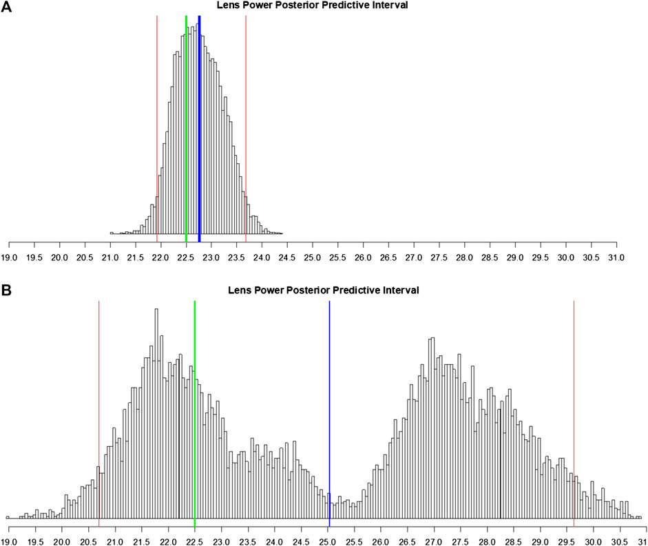
FIGURE 5. Histogram of posterior predictive samples for a random out-of-sample patient eye. The x-axis has the IOL values. The blue vertical line indicates the IOL prediction (mean of probabilities). The two red lines indicate the 95% predictive interval for IOL. The green line indicates the true lens power for this patient. (A) Posterior predictive sample for the eye with all measurements recorded. (B) Same as (A) except that many predictive variables were marked as missing.
To demonstrate the BART model’s flexibility in the case where the surgeon entered very little patient information, one of the major practical assets of our approach, we compare the situation where the outcome of this one eye is predicted with all measurements intact (Figure 5A) to the same eye where we deliberately omit some of the measurements and calculated variables (Figure 5B). Since it is the same eye, both scenarios share the real measured IOL power of 22.50 D in common.
With all measurements, the prediction is 22.76 ± 0.47 D with a 95% interval of [21.91 D, 23.70 D]. Note the shape of the posterior predictive distribution in Figure 5A: bell-like and symmetric (but not necessarily Gaussian); this is the usual scenario. This is a highly accurate estimate with a tight 95% uncertainty interval.
In the latter case, we consider the situation where the surgeon only recorded OD/OS, patient age, flat keratometry, steep keratometry, axial length, anterior chamber depth, SRK/T A-constant, and target post-operative spherical equivalent refraction. With many of our most predictive variables and calculated variables missing (see Explainability: Variable Importance), the BART model estimate of lens power is now 25.03 ± 2.86 D which is six times less accurate (in absolute deviation) than with all the measurements. Figure 5B shows that the 95% posterior predictive interval is now augmented to [20.69 D, 29.63 D], five times larger than previously. There is also an interesting bimodal shape to the posterior predictive distribution. This may signify that BART is fitting a mixture of two models (as visualized in the left hump and the right hump). As BART’s estimate is the mean of this bimodal distribution, the estimate falls in the center of these two humps, which is far from the true IOL power of 22.5, the center of the left hump.
In such a case, there is room for a clinician’s input. With more information, the ambiguity in which of the two models to select was resolved, with BART “picking” the correct one --- the model on the left (Figure 5A). The algorithm can thus advise the clinician to re-check patient measurement data and/or obtain measurements for the missing values among the 29 pre-op variables if applicable. In practice, our system can be used interactively. Note that there are no absolutely “required measurements” for our formula but there is great incentive (i.e., prediction accuracy) to collect as many as possible. In the case here, merely including variables from commonly used calculations (SRK/T A constant, Haigis, Holladay IOL, and Holladay ELP) disambiguates between these two models (in practice, our model does the computations of the 15 theoretical variables automatically). This reflects the fundamental target of our predictive model: the error in the calculated SRK/T modified IOL power.
We have demonstrated our formula’s effectiveness in our validated accuracy results which comes at the expense of low explainability (Explainability: Variable Importance). We now return to the question from the introduction: “Is there a downside in safety to using our high-generation machine learning formulas?”
We first have to answer how safety is related to accuracy. In cataract implant surgery, if the IOL power is predicted sufficiently wrong, the patient may have poor eyesight (“refractive surprise”) relative to the fellow eye. This can require the exchange of the intraocular lens or laser surgery. These post-operative fixes are not life-threatening and are mostly an annoyance. And, errors of this magnitude even when using lower-generation formulas are minimal, <0.1%. Hence, the bar of safety in this clinical setting is pretty low.
An error can come from two sources: (1) a measurement error i.e., an error in the measurement value of one of our inputs and (2) a prediction error in our formula. Source (1) is a problem for every single formula. Luckily, current biometry devices have self-correcting algorithms to insure proper variable acquisition. Surgeons are warned by the devices of values that are outside 3 standard deviations from the means. Thus, these errors are rare.
The more interesting error is source (2) i.e., an error that is the fault of our formula, the crux of our discussion. First, we never advocate herein for the clinician to robotically use our formula without their own input and other facts-on-the-ground that they judge are important via their clinical experience. They should consider our prediction formula within context of (1) a host of previous explicable formulas e.g., SRK/T and (2) the output of our uncertainty plots. If they judge our prediction to be sufficiently far from previous formulas and our uncertainty plot (Figure 5) to have large variance or multimodal shape, then they have to make their own judgment call. We repeat that our formula is as safe or safer than competing formulas in this context and that it meets current accepted FDA standards (FDA, 2020).
The raw data supporting the conclusions of this article will be made available by the authors, without undue reservation upon request to Clarke.
This study conformed to ethics codes based on the tenets of The Declaration of Helsinki and as the data are de-identified retrospective data; thus our study is exempted from IRB review under 45 CFR 46.101(b)(4). Written informed consent for participation was not required for this study in accordance with the national legislation and the institutional requirements.
GC owns copyright to the software described in this paper via his company Fullmonte Data, LLC. AK reported receiving wages for consulting for Fullmonte Data, LLC.
GC had full access to all the data in the study and takes responsibility for the integrity of the data collection. GC and AK performed the study concept and design, the analysis and interpretation of data, and the drafting of the manuscript.
Privately funded in a private clinic setting.
In addition to GC, the following surgeons provided data for this study: Dr. Jimmy K. Lee of the Albert Einstein College of Medicine, Dr. Cynthia Matossian of Matossian Eye Associates, Dr. Val Zudans and Dr. Karen Todd of the Florida Eye Institute, Dr. Thomas Harvey of the Chippewa Valley Eye Clinic, Dr. Stephen Dudley of OptiVision EyeCare, Dr. Paul Kang and Dr. Thomas Clinch of Eye Doctors of Washington, Dr. Paul (Butch) Harton of the Harbin Clinic, Dr. James Gills, Dr. Pitt Gills, and Dr. Jeffrey Wipfli of St. Luke’s Cataract and Laser Institute, and Dr. Ike Ahmed of the Prism Eye Institute.
Barrett, G. D. (1993). An improved universal theoretical formula for intraocular lens power prediction. J. Cataract Refract. Surg. 19 (6), 713–720. doi:10.1016/s0886-3350(13)80339-2
Bij, J. B., Edu, R., and Bennek, K. P. B. (2003). “Regression error characteristic curves,” in Proceedings of the Twentieth international conference on machine learning (ICML-2003), Washington, DC, August 21–24, 2003
Bleich, J., Kapelner, A., George, E. I., and Jensen, S. T. (2014). Variable selection for BART: an application to gene regulation. Ann. Appl. Stat. 8 (3), 1750–1781. doi:10.1214/14-aoas755
Box, G. E. P., and Draper, N. R. (2001). Empirical model-building and response surfaces. New York, NY: Wiley, Vol. 424.
Breiman, L. (2001). Statistical modeling: the two cultures (with comments and a rejoinder by the author). Stat. Sci. 16 (3), 199–231. doi:10.1214/ss/1009213726
Chipman, H. A., George, E. I., and McCulloch, R. E. (2010). BART: Bayesian additive regression trees. Ann. Appl. Stat. 4 (1), 266–298. doi:10.1214/09-aoas285
Clarke, G. P., and Burmeister, J. (1997). Comparison of intraocular lens computations using a neural network versus the Holladay formula. J. Cataract Refract. Surg. 23 (10), 1585–1589. doi:10.1016/s0886-3350(97)80034-x
Cooke, D. L., and Cooke, T. L. (2016). Comparison of 9 intraocular lens power calculation formulas. J. Cataract Refract. Surg. 2 (8), 1157–1164. doi:10.1016/j.jcrs.2016.06.029
FDA (2020). General principles of software validation. Available at: https://www.fda.gov/media/73141/download. (Accessed 12 June 2020).
Gökce, S. E., De Oca, I. M., Cooke, D. L., Wang, L., Koch, D. D., and Al-Mohtaseb, Z. (2018). Accuracy of 8 intraocular lens calculation formulas in relation to anterior chamber depth in patients with normal axial lengths. J. Cataract Refract. Surg. 44 (3), 362–368. doi:10.1016/j.jcrs.2018.01.015
Gelman, A., Carlin, J. B., Stern, H. S., and Rubin, D. B. (2003). Bayesian data analysis. Boca Raton, FL: Chapman & Hall/CRC, Vol. 2.
Haigis, W., Lege, B., Miller, N., and Schneider, B. (2000). Comparison of immersion ultrasound biometry and partial coherence interferometry for intraocular lens calculation according to Haigis. Graefes. Arch. Clin. Exp. Ophthalmol. 238 (9), 765–773. doi:10.1007/s004170000188
Hastie, T., and Tibshirani, R. (2001). The elements of statistical learning. Berlin, Germany: Springer.
Hoffer, K. J. (1993). The Hoffer Q formula: a comparison of theoretic and regression formulas. J. Cataract Refract. Surg. 19 (6), 700–712. doi:10.1016/s0886-3350(13)80338-0
Holladay, J. T., Musgrove, K. H., Prager, T. C., Lewis, J. W., Chandler, T. Y., and Ruiz, R. S. (1988). A three-part system for refining intraocular lens power calculations. J. Cataract Refract. Surg. 14 (1), 17–24. doi:10.1016/s0886-3350(88)80059-2
Kane, J. X., Van Heerden, A., Atik, A., and Petsoglou, C. (2017). Accuracy of 3 new methods for intraocular lens power selection. J. Cataract Refract. Surg. 43 (3), 333–339. doi:10.1016/j.jcrs.2016.12.021
Kapelner, A., and Bleich, J. (2015). Prediction with missing data via bayesian additive regression trees. Can. J. Stat. 43 (2), 224–239. doi:10.1002/cjs.11248
Kapelner, A., and Bleich, J. (2016). BartMachine: machine learning with bayesian additive regression trees. J. Stat. Software 70 (4), 1–40. doi:10.18637/jss.v070.i04
Keel, S., and van Wijngaarden, P. (2018). The eye in AI: artificial intelligence in ophthalmology. Clin. Exp. Ophthalmol. 47 (1), 5–6. doi:10.1111/ceo.13435
Norrby, S. (2008). Sources of error in intraocular lens power calculation. J. Cataract Refract. Surg. 34 (3), 368–376. doi:10.1016/j.jcrs.2007.10.031
Olsen, T. (2006). Prediction of the effective postoperative (intraocular lens) anterior chamber depth. J. Cataract Refract. Surg. 32 (3), 419–424. doi:10.1016/j.jcrs.2005.12.139
R Core Team (2018). R: A language and environment for statistical computing [computer program]. Version 3.5.0. Vienna, Austria: R Foundation for Statistical Computing.
Savini, G., Hoffer, K. J., and Barboni, P. (2015). Influence of corneal asphericity on the refractive outcome of intraocular lens implantation in cataract surgery. J. Cataract Refract. Surg. 41 (4), 785–789. doi:10.1016/j.jcrs.2014.07.035
Wang, L., Shirayama, M., Ma, X. J., Kohnen, T., and Koch, D. D. (2011). Optimizing intraocular lens power calculations in eyes with axial lengths above 25.0 mm. J. Cataract Refract. Surg. 37 (11), 2018–2027. doi:10.1016/j.jcrs.2011.05.042
Keywords: cataract surgery, intraocular lenses, intraocular lens power calculation formula, artificial intelligence, machine learning
Citation: Clarke GP and Kapelner A (2020) The Bayesian Additive Regression Trees Formula for Safe Machine Learning-Based Intraocular Lens Predictions. Front. Big Data 3:572134. doi: 10.3389/fdata.2020.572134
Received: 12 June 2020; Accepted: 30 October 2020;
Published: 18 December 2020.
Edited by:
Tuan D. Pham, Prince Mohammad bin Fahd University, Saudi ArabiaReviewed by:
Shivanand Sharanappa Gornale, Rani Channamma University, IndiaCopyright © 2020 Kapelner and Clarke. This is an open-access article distributed under the terms of the Creative Commons Attribution License (CC BY). The use, distribution or reproduction in other forums is permitted, provided the original author(s) and the copyright owner(s) are credited and that the original publication in this journal is cited, in accordance with accepted academic practice. No use, distribution or reproduction is permitted which does not comply with these terms.
*Correspondence: Gerald P. Clarke, Z3BjbGFya2UwNzI0QHlhaG9vLmNvbQ==; Adam Kapelner, a2FwZWxuZXJAcWMuY3VueS5lZHU=
Disclaimer: All claims expressed in this article are solely those of the authors and do not necessarily represent those of their affiliated organizations, or those of the publisher, the editors and the reviewers. Any product that may be evaluated in this article or claim that may be made by its manufacturer is not guaranteed or endorsed by the publisher.
Research integrity at Frontiers
Learn more about the work of our research integrity team to safeguard the quality of each article we publish.