 Sarah Van Driessche
 Kene Boun My
 Marielle Brunette3
94% of researchers rate our articles as excellent or good
Learn more about the work of our research integrity team to safeguard the quality of each article we publish.
Find out more
ORIGINAL RESEARCH article
Front. Behav. Econ., 11 September 2024
Sec. Behavioral Microfoundations
Volume 3 - 2024 | https://doi.org/10.3389/frbhe.2024.1456436
This article is part of the Research TopicDecision Making Under Risk and AmbiguityView all articles
Introduction: Ambiguity is part of most of the daily life decisions. It can affect the way people deal with environmental threats, especially when they face a social dilemma.
Method: We run an experiment where every group of four subjects is exposed to a risk that may result in a loss for each member. Subjects must decide on the allocation of their resources between mitigation strategies that allow them to decrease the probability of a disaster occurring for the group, and adaptation strategies that allow them to reduce the magnitude of that disaster for themselves only. In a first treatment (called Risk), subjects perfectly know the probability of occurrence of the event. We introduce ambiguity with regard to that probability in a second treatment (called Ambiguity), and in a third treatment (called Information Acquisition), subjects have the possibility to pay to obtain information allowing them to eliminate ambiguity.
Results and discussion: The results show that the introduction of ambiguity has no impact on average contributions compared to the Risk treatment. However, individual decisions to mitigate or to adapt are affected by subjects' attitude toward risk and ambiguity. In more than half of the cases, subjects are willing to pay to obtain information, which argues in favor of greater dissemination of information.
The last report of the Intergovernmental Panel of experts on IPCC (2021) emphasizes the urgent need to limit climate change. Societies must strengthen their mitigation efforts, just as they need to become more resilient by adopting effective adaptation policies. Dealing with climate change also comes with the uncertainties that surround this global issue which make it even more challenging (Bramoullé and Treich, 2009; Boucher and Bramoullé, 2010; Raihani and Aitken, 2011; Etner et al., 2020). Societal choices and actions implemented to tackle climate change in the immediate future will determine the next state of the world. The five Shared Socio-economic Pathways (SSP) scenarios of the IPCC are specifically designed to describe different plausible evolutions of the future society. Based on diverse socio-economic hypotheses and on different levels of greenhouse gas (GHG) emissions, they represent uncertain future situations. In this sense, these scenarios constitute a common basis to make decisions but are still ambiguous with regard to the likelihood of each one of them.1 Individuals are therefore not aware of the future climate conditions even though they need to address climate change promptly, through the implementation of mitigation and adaptation policies. This also raises the question of investments in more and better information in order to allay the uncertainties related to climate change (Ingham et al., 2007; Morath, 2010; Kuusela and Laiho, 2020).
In this ambiguous context, one may wonder what type of effort individuals are willing to make to cope with global warming. We consider that individuals may undertake two types of actions: mitigation or adaptation practices.2 Mitigation policies aim at curtailing the emissions of greenhouse gas in the atmosphere to lower the probability of bad climate states occurring (e.g., use of cleaner energy). Adaptation policies, however, serve to decrease the vulnerability of a person to the adverse consequences of climate change (e.g., installation of a drain system around one's house).3,4 It becomes apparent that mitigation can be compared to a global public good wherein each individual faces a cost to reduce GHG emissions while everyone can benefit from this reduction regardless of one's own contribution (Hasson et al., 2010, 2012). The trade-off between mitigation and adaptation therefore translates into a collective action problem. In addition to the conflicting interests between what is individually rational and what is socially optimal, risk and ambiguity preferences of people may also alter this choice. It is likely that decisions in terms of mitigation and adaptation change according to individual preferences.
In this paper, we propose to analyse how subjects deal with the threat of a climate event in a risky and in an ambiguous situation. For that purpose, we implement an experiment with context-framed instructions with students. The experimental design supposes a climatic risk that can entail a loss at the group-level (Hasson et al., 2010, 2012; Lefebvre and Van Driessche, 2022). In a first step, subjects are members of a group and they have to decide how much to invest in mitigation in order to reduce the probability of occurrence of the disaster for the whole group, and how much to allocate to adaptation in order to reduce the severity of the loss for themselves only. In the first treatment (Risk), subjects are in a risky situation. They know the probability of a climate event occurring. In the second treatment (Ambiguity), we introduce ambiguity with regard to the probability of occurrence of the event, so that subjects do not know in which state of nature they are. We also have a third treatment (Information Acquisition) in which we question subjects about their willingness to pay to obtain information, allowing them to go from an ambiguous context to a risky one. In a second step, subjects take individual decisions, which gives us a measure of their risk and ambiguity preferences.
Our paper is closely related to several other studies. Hasson et al. (2010, 2012) are the first to model the mitigation-adaptation trade-off as a public good experiment. Nevertheless, our experimental design differs from theirs in the sense that the authors consider a one-shot public good game with discrete choice. That is, subjects could choose to invest their whole endowment in either mitigation or adaptation but not in both measures at the same time. In a first paper, Hasson et al. (2010) study the impact of changing the vulnerability of subjects (i.e., the size of the climate event). They do not find any difference between the low-vulnerability and the high-vulnerability treatments. They explain this result by the role of trust (i.e., beliefs). In another paper, Hasson et al. (2012) compare a deterministic model (the climate hazard occurs with certainty) and a stochastic one (there is a risk of a climate event occurring). The results indicate that there is no difference between the two models in terms of mitigation and that the level of cooperation is rather low. Lefebvre and Van Driessche (2022) experimentally examine the effects of income inequality on the mitigation-adaptation trade-off. They find out that group contributions are not affected by the degree of inequality. McEvoy et al. (2022) look at the effect of non-binding pledges when subjects only have the possibility to mitigate, and when they can both mitigate and adapt. Their results suggest that pledges increase mitigation contributions only when both climate policies are available. Blanco et al. (2020) also study social dilemmas but in a wider context than climate change. Subjects are given three possibilities to face potential losses at the group-level: public insurance (reduction in the group probability), private insurance (reduction in the individual size of the loss), and no insurance (increase in the individual payoff). They investigate the impact of varying the size of the loss and find that investments in public insurance decrease as this size decreases. Keser and Montmarquette (2008) examine the behavior of group members who can collectively contribute to reduce the probability of a common loss. They show that introducing ambiguity has a negative impact on the level of voluntary contributions.
There is, however, a growing body of literature which considers adaptation as a global public good. Khan and Munira (2021) argue that reframing adaptation as a global public good would be beneficial for its funding. Adaptation has long been regarded as a local or national good which has led to insufficient financial backing. Yet, adaptation measures provide indirect benefits such as maintaining world trade, reducing migratory flows, avoiding pandemics, etc., which are likely to benefit everyone (Kartha et al., 2006). Banda (2018) considers adaptation as a multi-level (i.e., domestic, transboundary, and global) public good. She explains that, given this particularity, the unilateral effort of individual nations will not be enough to ensure the provision of this good. It will require international legal and governance frameworks as well as a more consistent adaptation finance. Nevertheless, for this experiment, we consider adaptation as a private action so as to confront subjects with a social dilemma.
This paper is also related to another strand of the literature, namely public good games with uncertainty. There is no clear picture that emerges from that literature. Some experiments have focused on introducing uncertainty about the marginal per capita return (see e.g., Fisher et al., 1995; Levati et al., 2009; Fischbacher et al., 2014; Bjök et al., 2016; Boulu-Reshef et al., 2017; Théroude and Zylbersztejn, 2020), while others have looked at the effect of introducing uncertainty about actually receiving the benefits from the public good (see e.g., Dickinson, 1998; Gangadharan and Nemes, 2009; Levati and Morone, 2013). Fisher et al. (1995), Bjök et al. (2016), Boulu-Reshef et al. (2017), and Théroude and Zylbersztejn (2020) find no effect of uncertainty on the level of contributions. However, Gangadharan and Nemes (2009), Levati et al. (2009), and Fischbacher et al. (2014) show evidence of a negative effect on cooperation. Levati and Morone (2013) state that this negative impact is due to the payoff parameterization. Other papers have looked at the effect of uncertainty in threshold public good games. In this kind of games, the provision of the public good must attain a certain level in order to avoid a collective loss. Barrett and Dannenberg (2012, 2014) introduce uncertainty regarding the location of the threshold, that is, the threshold lies within a known range of values. Dannenberg et al. (2015) consider an ambiguous threshold. The results show that cooperation is hindered by uncertainty and even more by ambiguity.
The role of risk and ambiguity preferences has also been carefully studied in the economic literature.5 Risk aversion has long been recognized as a key determinant of individual behaviors (Pratt, 1964). Its effect on various decisions has been considered: insurance (Mossin, 1968), self-insurance and self-protection (Ehrlich and Becker, 1972), the level of effort (i.e., preventing activity) (Jullien et al., 1999), timber harvesting (Brunette et al., 2017b), etc. In particular, De Pinto et al. (2013) show that considering risk neutral farmers whereas they are risk averse leads to miscalculate the incentives required to induce participation to a mitigation policy, like carbon sequestration programs. Truong and Trück (2016) show that assuming risk neutrality rather than risk aversion results in an unnecessary delay of investments in adaptation policies. However, Lades et al. (2021) questioned the capacity of different economic preferences (i.e., risk taking, patience, present bias, altruism, negative and positive reciprocity, and trust) to predict pro-environmental behaviors in everyday life. They found that altruism is the only preference which is related to environmentally friendly attitudes. This suggests that individuals do not consider or do not perceive the inherent riskiness of environmental decisions. They rather focus on the pro-social aspects of pro-environmental behaviors.
Regarding ambiguity preferences, Ellsberg (1961) is the first to identify this tendency to avoid ambiguous situations and to prefer risky ones. As for risk preferences, ambiguity aversion has been widely considered to characterize numerous individual decisions: value of a statistical life (Treich, 2010), portfolio choices (Gollier, 2011), insurance and self-protection (Alary et al., 2013), etc. Especially, Berger et al. (2017) show how ambiguity aversion influences the optimal level of mitigation. They proposed an integrated assessment model that generates quantitative estimates of the impact of ambiguity aversion on optimal emissions reduction. Brunette et al. (2017a) analyse the relevancy of considering adaptation efforts in an insurance contract to lower the financial cost of the insurance premium when climate change makes the probability of the natural event occurring uncertain. They show that including adaptation efforts in the insurance contract leads to an increase in the adaptation efforts of risk-averse and ambiguity-averse agents. In the same vein, Brunette et al. (2020), combining an elicitation method and survey questions, show that risk aversion has a significant and negative impact on the probability to adapt and on the intensity of adaptation, whereas ambiguity aversion has no effect. Alpizar et al. (2011) study the role of ambiguity aversion in the choice to adapt to climate change. By means of a framed field experiment with coffee farmers in Costa Rica, they find that ambiguity aversion fosters the adoption of technologies for adaptation.
Preferences toward risk and ambiguity have been found to explain various individual choices and, in particular, mitigation and adaptation decisions. Our study aims at looking at the effects of these preferences on the choice of one strategy or the other. To the best of our knowledge, this is the first experiment that examines the trade-off between mitigation and adaptation by considering a risky context and an ambiguous one. Anticipating our results, we find that: (i) there is no difference in average contributions between the Risk and Ambiguity treatments; (ii) risk and ambiguity preferences impact the decisions to mitigate or to adapt; (iii) ambiguity preferences explain the willingness to pay to obtain information.
The rest of the paper is organized as follows. In Section 2, we present the experimental design. In Section 3, the results are described. Section 4 provides a discussion of the results and concludes.
The experiment consists of a repeated game played for ten periods. Subjects are divided into groups of four. The groups remain unchanged throughout all the periods of the game. At the beginning of each period, subjects receive an endowment of 250 ECUs6 (Experimental Currency Units) that allows them to recover from a potential loss of 200 ECUs, and a climate budget of 25 tokens which has to be entirely spent on the two strategies (i.e., mitigation and adaptation). Following Hasson et al. (2010, 2012), we do not give subjects the opportunity to “do nothing,” that is, to ignore threats from climate change and keep their tokens for themselves. While the experiment would gain in external validity with that third option, it would also prevent us from analyzing the real-life trade-off between adaptation and mitigation in the management of threats. Indeed, if most of the subjects preferred this third option, there would be no trade-off to analyze and therefore we would be unable to address our research question.
In each period, every group faces a risk of incurring a climate-related event that can inflict a loss of 200 ECUs on each member. Subjects must decide, at the same time and without communicating with each other, on the allocation of their climate budget between adaptation and mitigation strategies. Relying on Alekseev et al. (2017), we use context-framed instructions in order to ease the comprehension of the tasks for the subjects and avoid confusion. Thus, rather than using abstract terms, we employ words like “climate change,” “mitigation,” “greenhouse gas,” etc., which are supposed to be more evocative (see the instructions in the Supplementary material). At the beginning of the game, we ask subjects to imagine that they are part of a small community which is threatened by climate-related events (such as rising water leading to floods, extreme heat waves, storms, etc.). We also give them concrete examples of the two strategies. We explain that mitigation actions can consist in sorting and reducing waste or choosing public transport rather than the car to move around. We illustrate adaptation by replacing the windows with laminated glass in order to face high winds. However, still in an attempt to facilitate the understanding of the game, we explain that the occurrence of a climate event depends on a random draw of a ball from an urn filled with balls of two different colors.
The climate budget must be divided between mitigation and adaptation. A token invested in mitigation reduces the probability of the climate event occurring for all the group members. This probability is represented by an urn filled with black balls (event) and white balls (no event). Depending on the treatment (see below), we use either one or all of the following mitigation urns:
• Urn A contains a total of 150 balls. It is initially comprised of 145 black balls and five white balls, such that the initial occurrence probability equals 96.7%.
• Urn B contains a total of 150 balls. It is initially comprised of 125 black balls and 25 white balls, such that the initial occurrence probability equals 83.3%.
• Urn C contains a total of 150 balls. It is initially comprised of 105 black balls and 45 white balls, such that the initial occurrence probability equals 70%.
Every token contributed to mitigation replaces a black ball with a white ball in the urn, thus it reduces the probability by 0.67%. Therefore, the probability decreases as group members allocate their tokens to mitigation and is given by the following function:
where xi is the number of tokens contributed to mitigation by subject i, i∈{1, 4}, and Bu is the initial number of black balls in the mitigation urn (u = A, B, C).
However, a token allocated to adaptation reduces the size of the potential loss only for the individual who decides to adapt. The reduction of the loss follows this linear function:
where (25−xi) represents the number of tokens invested in adaptation by subject i. In order to help subjects make their decisions, a table displaying the amount of the loss for every token invested in adaptation was included in the instructions (see the Supplementary material).
While the marginal benefit of a token contributed to mitigation does not depend on the urn, the marginal cost (i.e., giving up on the possibility to reduce the size of the damage) does. The higher the occurrence probability of the climate event, the higher the marginal cost of a token invested in mitigation. A risk-neutral and self-interested subject has two strategies to maximize their payoffs which depend on the number of tokens the other group members invest in mitigation. As long as there are strictly less than:
• 69 tokens invested in mitigation in urn A,
• 49 tokens invested in mitigation in urn B,
• 29 tokens invested in mitigation in urn C,
the marginal benefit of a token allocated to mitigation is always lower than the marginal cost. Therefore, the subject should not invest in mitigation. When the mitigation fund exceeds the aforementioned levels, the subject should invest all their tokens in mitigation.
The random draw of a ball by the computer arises at the end of each period. We acknowledge that it would make more sense in terms of external validity to consider that the benefits of mitigation occur in the long term (i.e., a few periods later). However, it would mean considering a dynamic public good game which is outside the scope of this paper.
In this subsection, we present the three different treatments implemented in this experiment: Risk (hereafter R), Ambiguity (hereafter Amb), and Information Acquisition (hereafter IA).
In the Risk treatment (R), subjects are in a risky situation. They face the mitigation urn B. They know the initial composition of the urn and are thus aware that if no token is contributed to mitigation, the probability of an event occurring for the group is 83.3%, while if the four group members invest their entire climate budget in mitigation, the probability decreases down to 16.7%.7 In order to facilitate the subjects' decision making, we give them access to two sliders. The first one allows them to simulate their own level of contribution to mitigation, while the second one represents the total investment of the three other group members. According to the position of the sliders, the resulting probability is displayed in a pie chart (see Figure 1).
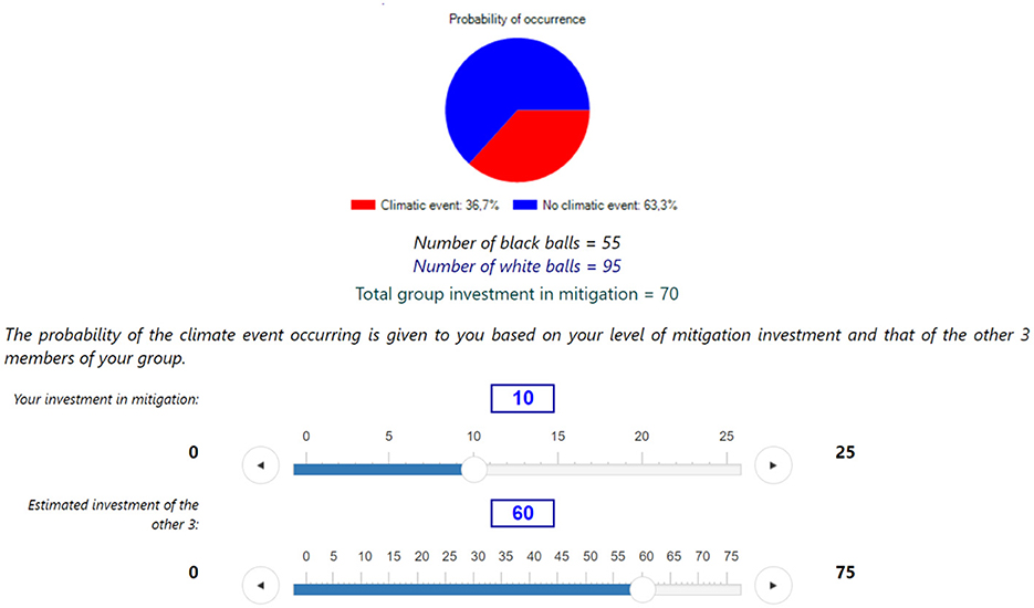
Figure 1. Resulting probability in risk (screenshot).
In the Ambiguity treatment (Amb), subjects are in an ambiguous situation with regard to the probability of a climate event occurring. Indeed, they face the three mitigation urns (A, B, C) without knowing which one will be selected. They make their allocation decisions considering the three different possible states of nature, with urn A representing the most adverse state and urn C corresponding to the most favorable one. They are aware of the initial composition of each urn, so that they know that the probability of:
• Urn A goes from 96.7% if no one contributes to mitigation, to 30% if the four group members invest their 25 tokens in mitigation.
• Urn B goes from 83.3% if no one contributes to mitigation, to 16.7% if the four group members invest their 25 tokens in mitigation.
• Urn C goes from 70% if no one contributes to mitigation, to 3.3% if the four group members invest their 25 tokens in mitigation.
In order to facilitate the subjects' decision making, they also have access to the two sliders in order to simulate their own level of contribution to mitigation and the total investment of the three other group members. According to the position of the sliders, the resulting probability for each mitigation urn is displayed in a pie chart (see Figure 2).
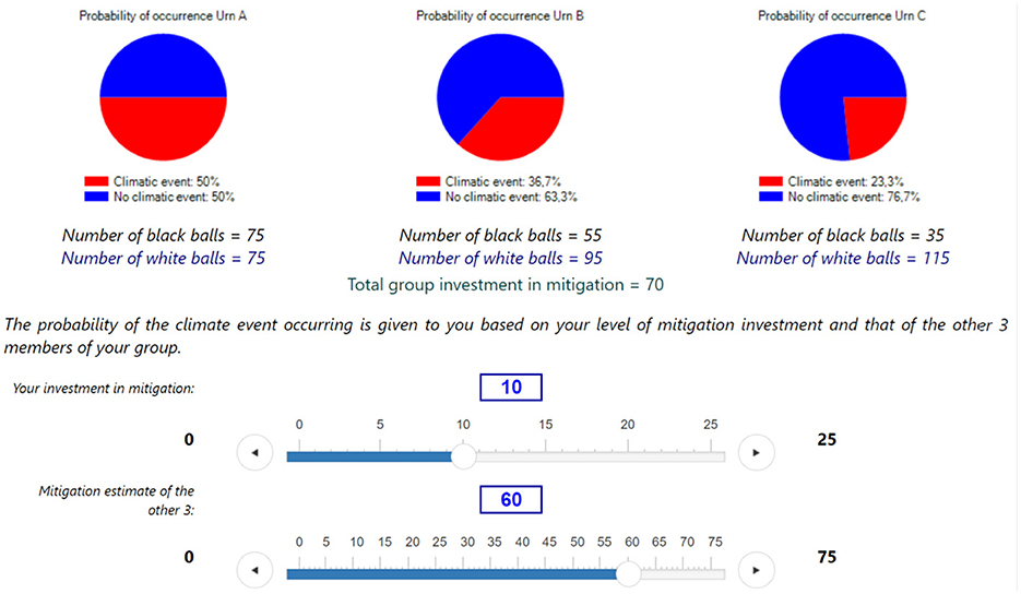
Figure 2. Resulting probabilities in Ambiguity (screenshot).
Following Attanasi et al. (2014), we use a two-stage lottery to determine the occurrence of a climate event. To that end, in each period, an opaque big urn which contains one hundred mitigation urns of three different compositions (urn A, urn B, and urn C) is generated. Subjects do not know the proportion of urns A, B and C in the big urn nor the mitigation urn which is randomly drawn from the big opaque one. Therefore, they do not precisely know the probability of a climate damage occurring in the Ambiguity treatment.
In the Information Acquisition treatment (IA), subjects are initially confronting the three mitigation urns and they have the possibility to buy information in order to know which of the three urns they will actually face. To do so, they can use up to 50 ECUs from their endowment of 250 ECUs.8 Subjects are asked to indicate the maximum price at which they are willing to buy information about the selected urn.9 This price should give us an approximation of the subjects' Willingness To Pay (WTP) to eliminate ambiguity, and thus to make their decision in a risky context rather than in an ambiguous one. In every period, the computer randomly generates a number for each group which determines the actual price of information. If the price indicated by a subject is equal to or higher than the one set by the computer, the subject learns the selected mitigation urn and pays the computer's price. Otherwise, the subject does not get information and pays nothing.10
In each treatment, subjects make the same decision, that is, they decide how many tokens they want to allocate to mitigation and how many they want to invest in adaptation. In the Amb and IA treatments, prior to this decision, subjects have to indicate which urn they think they will face (A, B, C, or “I do not know”). Then, in IA, subjects must reveal their willingness to pay to obtain information. If they get information, they take their allocation decision in a risky context, facing either urn A, B, or C. If they do not receive information, they make their decision in an ambiguous context (as in Amb). Regardless of the treatment condition, subjects also have to declare how many tokens they think the three other members will invest in mitigation. Following Gächter and Renner (2010) and Blanco et al. (2010), we incentivize subjects' beliefs. They are rewarded according to the precision of their beliefs. They earn 25 additional ECUs if they correctly (±7 tokens) predict the total investment of the three other members.
The gains of subjects, for each period, depend on whether or not an event occurs. It is determined by a random draw of a ball (black or white) from the mitigation urn B in R and from the selected mitigation urn (i.e., either A, B, or C) in Amb and IA. If there is a climate event, in R and Amb, subjects get their endowment of 250 ECUs minus the amount of the loss whose size depends on their investment in adaptation. In IA, they get their endowment of 250 ECUs minus the amount of the loss, minus the price of information if they had access to it. If no climate damage occurs, in R and Amb, subjects get their endowment of 250 ECUs, and in IA, they receive their endowment of 250 ECUs minus the price of information if they got it.
At the end of each period, subjects are informed of the drawn urn in Amb and IA, the total investment of their group in mitigation, the resulting probability, the occurrence of the climate event, and their own payoffs.
After the ten periods of the main game, we use two questionnaires to assess the environmental sensitivity of subjects. The first one investigates subjects' pro-environmental behaviors. They must answer to the fifteen statements by indicating the frequency (between 1 “never” and 5 “always”) with which they adopt pro-environmental attitudes (see the instructions in Supplementary material). The second one is the New Ecological Paradigm (NEP) scale (Dunlap et al., 2000). It aims to assess the ecological consciousness of subjects. They have to indicate (using a Likert scale from 1 “strongly disagree” to 5 “strongly agree”) whether or not they agree with the fifteen sentences regarding limits to growth, anti-anthropocentrism, fragility of balance, rejection of exemptionalism, and ecocrisis (see the instructions in Supplementary material).
We also measure Social Value Orientation (SVO) of subjects following Murphy et al. (2011).11 To do so, subjects are randomly grouped in pairs and have to decide how they want to allocate resources between themselves and the other person. For the six different propositions, subjects must indicate which distribution of resources they prefer (see the instructions in Supplementary material). According to their answers to the six propositions, it is possible to classify them into four categories: altruist, prosocial, individualist, and competitive (we use them as explanatory variables in the regressions, see below).
Finally, following Halevy (2007), we ask subjects for their certainty equivalent of two lotteries: a known lottery and an unknown lottery.12 This allows us to elicit subjects' risk and ambiguity attitude within a Klibanoff et al. (2005) (KMM) framework. Before completing these two tasks, subjects have to select their winning color (yellow or blue). In the first task, they must choose between a lottery with known probabilities (represented by an urn comprised of five yellow balls and five blue balls, Lknown) and ten fixed amounts of money. More specifically, they have to make a choice between the Left option which is a lottery with two outcomes (0€and 10€) and 50% chance of getting either 0€or 10€, and the Right option which provides a safe amount of money, from 1€in the first proposition, 2€in the second one, to 10€in the tenth one (see the instructions in Supplementary material). For the ten propositions, subjects have to indicate whether they prefer the Left or the Right option.13 Then, we use the subjects' switching point between the two options to classify them as either risk averse, risk neutral or risk lover (we use this classification in the regressions, see below). Similarly, in the second task, subjects also have to choose between the Left and the Right option. The only difference is that they do not know the composition of the urn. Therefore, they have to decide between a lottery with two outcomes (0€and 10€) and unknown probabilities (Lunknown), and a sure amount of money, from 1€in the first proposition, 2€in the second one, to 10€in the tenth one (see the instructions in Supplementary material). Relying on d'Albis et al. (2020), we use their definition of value-ambiguity attitude in order to classify subjects into three categories: value-ambiguity averse, value-ambiguity neutral, and value-ambiguity lover (we use them as explanatory variables in the regressions, see below). To do so, we compare the subjects' switching point for the known lottery (Lknown) and the unknown lottery (Lunknown).
A total of 192 subjects participated in 12 sessions (four sessions per treatment) in September, October and November 2021 in Strasbourg and in Nancy. Each subject participated in one treatment only. Half of the subjects were recruited from a list of experimental subjects maintained at the Laboratory of Experimental Economics of Strasbourg (LEES) using the ORSEE software (Greiner, 2015). We contacted the other half by mail because we targeted students who were pursuing environmental studies. Since those students are supposed to be more committed to the environmental cause, we wanted to see whether they would behave differently than students from other disciplines. Therefore, three sessions were run with students from the National School for Water and Environmental Engineering of Strasbourg (ENGEES) and three others with students from AgroParisTech (APT) in the campus of Nancy. Apart from the location, the conditions of the experiment were the same for each session. Table 1 summarizes the number of sessions and subjects per treatment for all subjects (All) and for the two subcategories of subjects: subjects whose studies are not specifically environment-related (hereafter called Classic) and those who pursue environmental studies (hereafter called Environment).14 The latter category corresponds to the students from ENGEES and APT.
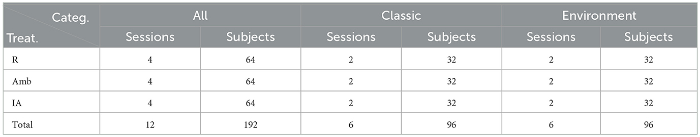
Table 1. Number of sessions and subjects per treatment.
All subjects completed the experiment using tablet computers. Each session followed an identical procedure. The instructions were read aloud by the experimenter and, before starting, subjects had to respond to a comprehension questionnaire in order to check that they properly understood the rules. The experiment could start only after all subjects had cleared the control questions. After the ten periods of the main game, subjects completed the questionnaire about their environmental habits and the NEP. The last parts of the experiment consisted of the SVO and the elicitation of risk and ambiguity preferences. Finally, subjects answered a post-experiment questionnaire (see the instructions in Supplementary material).
At the end of the experiment, one period from the main game was randomly selected for actual payment. For the SVO, a random draw was made to determine which of the six propositions would actually be paid out. Either the risk elicitation task or the ambiguity elicitation task was rewarded and it also depended on a random draw. Independently of the task selected at random, the computer selected the proposition which would be compensated. If, for that proposition, a subject chose the Left option, then the computer randomly drew a ball from the urn. If the ball was the same color as the subject's winning color, the subject got 10€. Otherwise, the subject got 0€. However, if a subject chose the Right option, the subject got the amount corresponding to the proposition selected by the computer. The conversion rate was 100 ECUs to 4€for the main game and the SVO. Subjects were paid their earnings privately at the end of the session. A session lasted 100 min on average and the average earnings were 20.85€ (SD = 4.77). The next section presents the results.
Recall that subjects have a climate budget of 25 tokens to fully allocate between mitigation and adaptation. We choose to consider, as our variable of interest, the amount of tokens contributed to the mitigation measure. However, the opposite results are true for adaptation. We proceed in two steps to analyse the results. First, we focus on average contributions to mitigation, then we study the individual decisions to mitigate or to adapt and we run a series of regressions.
In the second column of Table 2, we present the average contributions to mitigation per treatment for all subjects (All) and for the two subcategories of subjects (Classic and Environment). In the Risk treatment, the average contribution amounts to 17.28 tokens which represents 69.12% of the climate budget. This figure is relatively high compared to the initial average contribution of 40%–60% usually observed in traditional public good games (Villeval, 2012). Moreover, we do not see a decline in average contributions over time for the two subcategories of subjects, as illustrated in the top-left corner of Figure 3. Unlike traditional public good games, recall that zero contribution is not a dominant strategy in R. Subjects may have an interest in investing all their tokens in mitigation, depending on the number of tokens in the mitigation fund. This can explain why subjects maintain cooperation throughout the periods of the game, and thus why our results depart from what is generally seen in public good games. The same observation is true in Amb. Subjects invest on average 16.49 tokens in mitigation, that is, 65.96% of their climate budget. The top-right corner of Figure 3 also shows no decrease in mean contributions over time for the two subcategories of subjects.
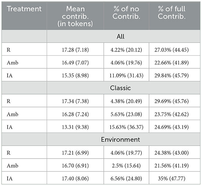
Table 2. Mean (in tokens), minimum and maximum (in %) contributions to mitigation (SD in parentheses).
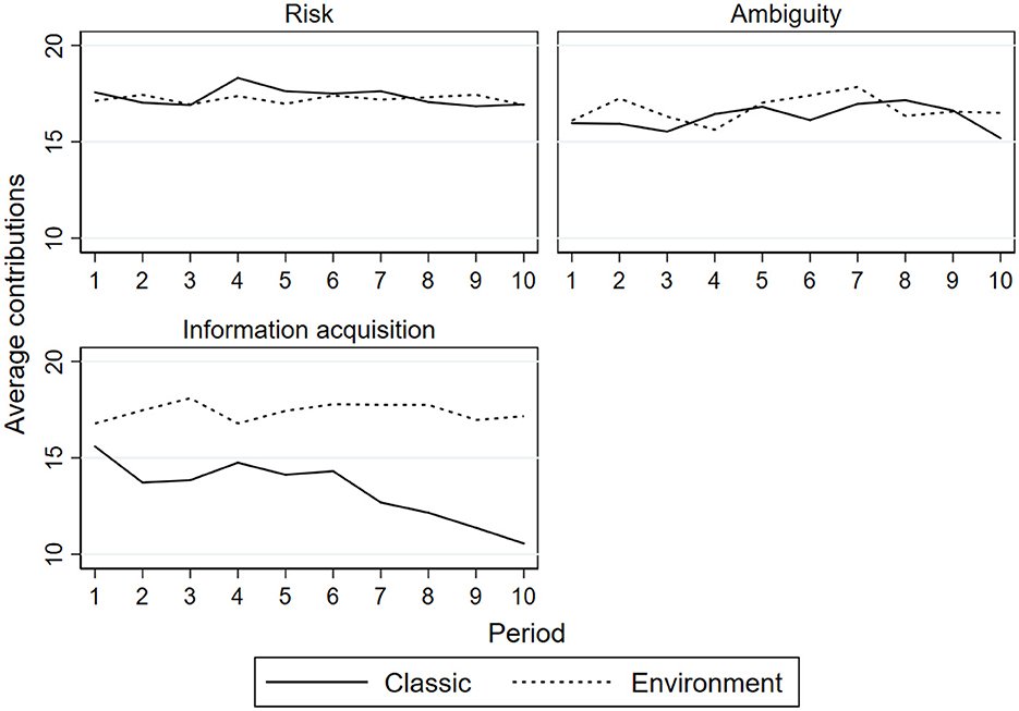
Figure 3. Mean contributions to mitigation over period per treatment.
In order to assess the effect of introducing ambiguity in the game, we now compare the Risk and Ambiguity treatments.15 For the whole sample of subjects, in R, average contributions equal 17.28 tokens and in Amb, subjects invest on average 16.49 tokens. However, this difference is not significant according to a two-sided Mann-Whitney (MW) ranksum test taking group averages as units of observation (p = 0.4177).16 The same holds true for Classic subjects. There is no significant difference in average contributions between R (17.34) and Amb (16.28; p = 0.5632). For Environment subjects, mean contributions in R (17.21) and in Amb (16.70) are not statistically different either (p = 0.5992). In the public good games' literature, a series of papers that attempts to assess the effect of uncertainty about the marginal per capita return also finds zero effect on contributions (see e.g., Fisher et al., 1995; Boulu-Reshef et al., 2017; Théroude and Zylbersztejn, 2020). It should be noted that looking at average contributions does not allow us to identify the effect of individual preferences. This will be studied in subsection 3.2 when looking at individual decisions. It ensues from the above the following result.
RESULT 1. Introducing ambiguity with respect to the probability of a climate-related event occurring does not affect average contributions to mitigation.
Then, we compare Classic and Environment subjects. We only find a marginally significant difference in mean contributions in the Information Acquisition treatment (p = 0.0929). The results suggest that Classic subjects invest less on average (13.31) than Environment ones (17.40). There is no significant difference for the other treatments.17
In the last two columns of Table 2, we also report the percentages of time subjects do not invest in mitigation (0 token contributed) and the percentages of time they contribute their entire climate budget (25 tokens) per treatment and for the different categories of subjects. If we consider the Risk and Ambiguity treatments, we see that, for the whole sample of subjects (All), the percentages of zero contribution are around 4% (respectively 4.22 and 4.06%, p = 64.17).18 Regarding the proportions of maximum contributions, subjects invest all their tokens 27.03% of time in R and 22.65% of time in Amb. The difference is not statistically significant (p = 0.6056).19 For Classic subjects, the proportion of minimum contributions in R (4.38%) is not statistically different from this proportion in Amb (5.63%; p = 0.9764). The same holds true for the percentages of full contributions, there is no difference between R (29.69%) and Amb (23.75%; p = 0.6842). If we now look at Environment subjects, there is no difference in the percentages of zero contribution between R (4.06%) and Amb (2.5%; p = 0.4492), nor is there a difference in the proportions of full contributions between R (24.38%) and Amb (21.56%; p = 0.7539). On the basis of the above, we formulate the next result.
RESULT 2. Introducing ambiguity has no effect on the proportions of minimum and maximum contributions.
Between the two subcategories of subjects, the only difference lies in the proportions of minimum contributions in IA. Classic subjects tend to contribute 0 token more often (15.63%) than Environment ones (6.56%; p = 0.0119). This may provide an explanation as to why average contributions seem to be lower for Classic subjects than for Environment ones in IA. The bottom-left corner of Figure 3 which represents the average contributions to mitigation per period for the two subcategories of subjects, shows that average contributions of Classic subjects tend to decrease over time, especially in the last periods of the game. Data analysis shows that the number of free-riders (who invest 0 token in mitigation) doubled in the last three periods of the game.20
Remember that, in the IA treatment, subjects have the possibility to buy information in order to know which urn they will face. The average contribution, in this treatment, amounts to 15.35 tokens (see Table 2). For the analysis, we distinguish between subjects who wish to obtain information about the selected urn (i.e., WTP >0) and those who do not (i.e., WTP = 0) (respectively wish yes/wish no). We also identify subjects who actually get information (i.e., WTP ≥ price) and those who do not (i.e., WTP < price) (respectively info yes/info no). The first panel of Table 3 summarizes the number of times subjects wish to receive information and the number of times they get it, as well as their willingness to pay to eliminate ambiguity. In 52.97% of the cases, subjects wish to obtain information. In particular, Classic subjects wish to get information in 56.25% of the cases and Environment subjects wish to obtain it in 49.69% of the cases. The difference between Classic and Environment subjects is not statistically significant according to a MW ranksum test taking the number of times individuals wish to obtain information as units of observation (p = 0.4590). Subjects actually get information in 21.88% of the cases: 17.5% for Classic subjects and 26.25% for Environment subjects. The difference between Classic and Environment subjects is not statistically significant according to a MW ranksum test taking the number of times individuals receive information as units of observation (p = 0.4379).
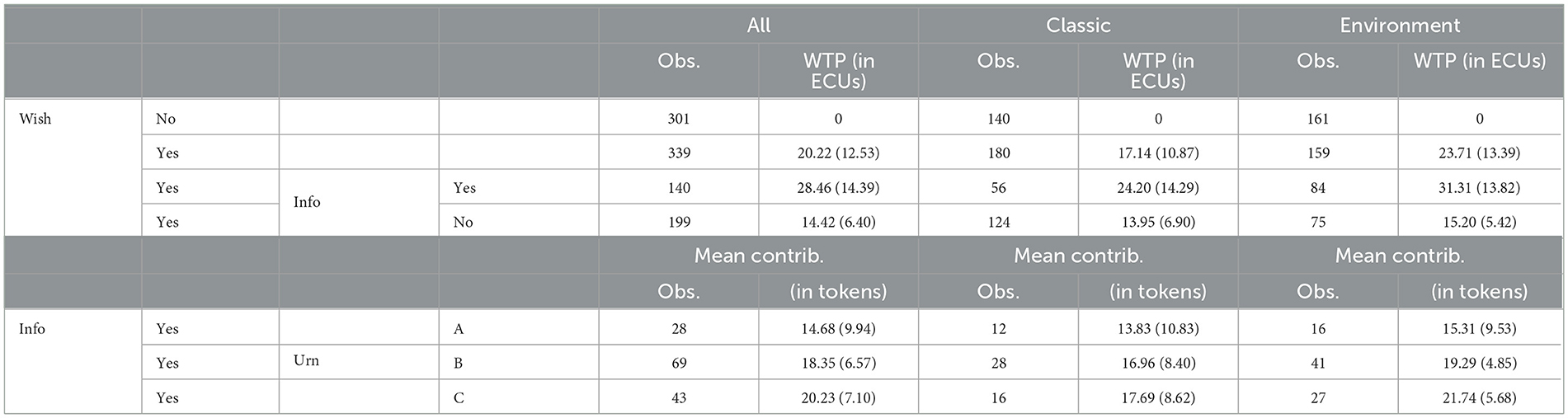
Table 3. WTP (in ECUs) and mean contributions (in tokens) according to the urn (SD in parentheses).
Regarding the WTP of subjects, Classic subjects offer on average 9.64 ECUs (SD = 10.98) to obtain information and Environment subjects offer 11.78 ECUs (SD = 13.92).21 However, the difference is not statistically significant according to a MW test taking individual averages as units of observation (p = 0.8759). We can see from Figure 4 which represents the distributions of the WTP for the two categories of subjects, that the mode of both distributions is 0 (43.75% for Classic subjects and 50.31% for Environment subjects). A Kolmogorov–Smirnov test taking individual averages as units of observation indicates that the two distributions are not statistically different (p = 0.968). If we only consider strictly positive offers, the average WTP of Classic subjects equals 17.14 ECUs (34.28% of the 50 ECUs) and it amounts to 23.71 ECUs (47.42% of the 50 ECUs) for Environment subjects. On the basis of the above, we present the next result.
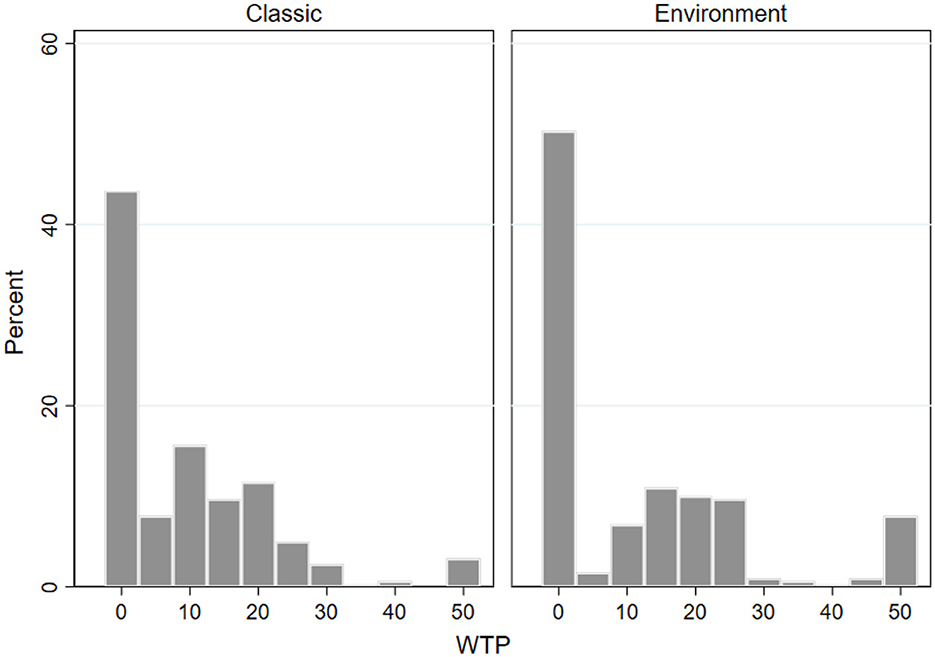
Figure 4. Distributions of WTP (in ECUs) for Classic and Environment subjects.
RESULT 3. Classic and Environment subjects do not behave differently in IA.
In the second panel of Table 3, we look at the average number of tokens subjects contribute to mitigation when they get information about the selected urn. Subjects invest the least in mitigation (14.68) when they face urn A (unfavorable state). Classic subjects contribute 13.83 tokens on average and Environment subjects invest 15.31 tokens. Mean contributions are higher when subjects are aware that urn B is drawn (18.35). Classic subjects invest an average of 16.96 tokens and Environment subjects contribute 19.29 tokens on average. When urn C is selected (favorable state), mean contributions are the highest (20.23). Classic subjects invest 17.69 tokens on average and the mean contribution of Environment subjects is 21.74 tokens. It seems that subjects use the information they receive and that they mitigate more when they are in the most favorable state (urn C).
We now turn to the analysis of individual decisions in order to look at the determinants of the choice to mitigate or to adapt in the different treatments. We estimate tobit models with random effects since the dependent variable (the number of tokens invested in mitigation) is left-censored at 0 and right-censored at 25. Table 4 presents the different variables that are used in the regressions along with some descriptive statistics and the results are presented in Tables 5, 6.
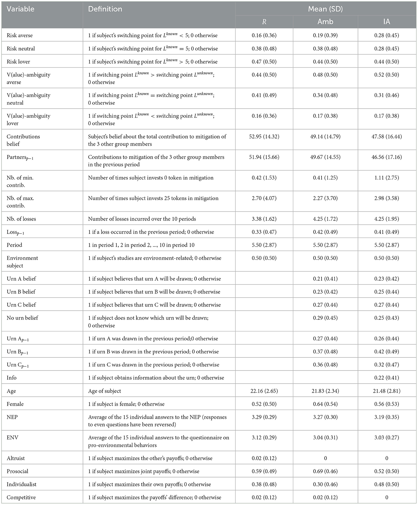
Table 4. Variables definition and descriptive statistics per treatment.
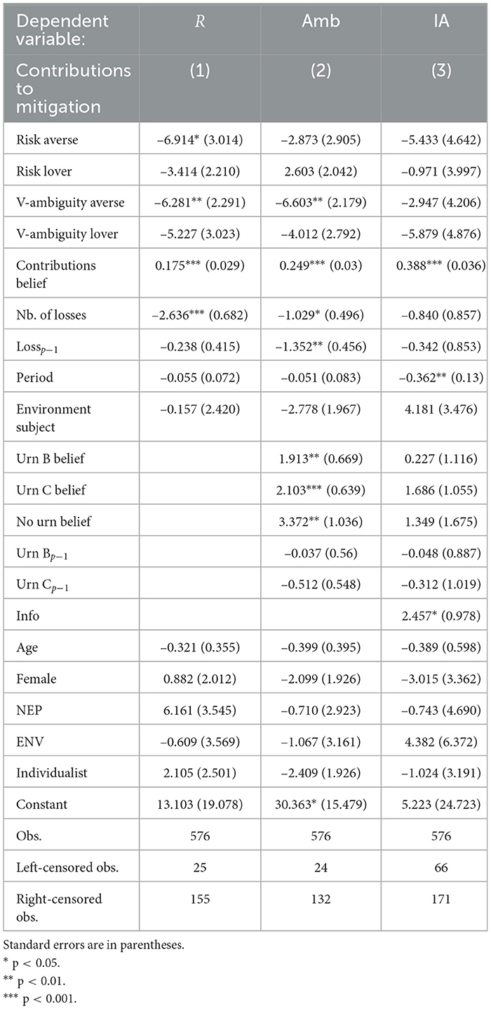
Table 5. Tobit regressions per treatment.
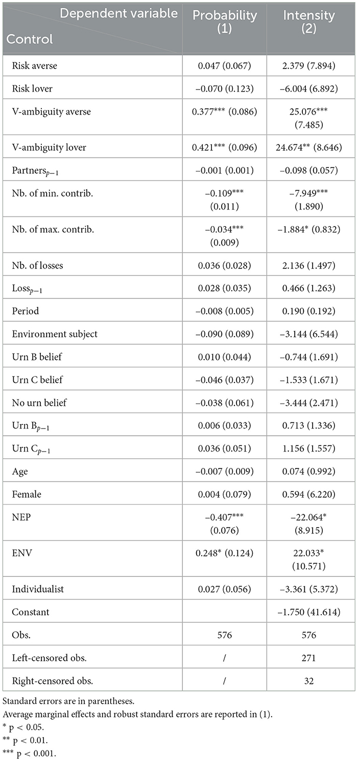
Table 6. Probit and tobit regressions on the WTP in IA.
Specification (1) of Table 5 focuses on the Risk treatment. In this treatment, the subjects' preferences toward risk and ambiguity play a role in the decision to mitigate or to adapt, as evidenced by the coefficients of Risk averse and V-ambiguity averse22 which are statistically significant and negative. For risk averse subjects facing urn B, zero contribution can become a dominant strategy depending on their degree of risk aversion if we consider the Constant Relative Risk Aversion utility function. Indeed, risk averse subjects need a higher level of investment in mitigation than risk neutral subjects (whose level is 49) in order to have an interest in investing all their tokens in mitigation. This can explain why risk averse subjects invest less than risk neutral subjects. Value-ambiguity aversion also has a negative effect on mitigation investments, even though there is no ambiguity per se in this treatment. However, there is strategic ambiguity which refers to situations where the behaviors of others cannot be precisely predicted (Eddai and Guerdjikova, 2023). Gangadharan and Nemes (2009) studied the effects of strategic and environmental uncertainty on the provision of public and private goods. The authors found evidence of aversion from strategic uncertainty, that is, even when subjects know that either the probability of return from the private good is low or the probability of return from the public good is high, they prefer to invest their tokens in the private good. In our case, strategic uncertainty matters a great deal since the strategy of a particular subject depends on what the others will do. This may explain why value-ambiguity averse subjects prefer to adapt more than value-ambiguity neutral subjects. Among other results, we see that the coefficient of Contributions belief is positive and significant. In a similar experiment, Lefebvre and Van Driessche (2022) found the same result. This is a well-known result in public good games. Fischbacher and Gächter (2010) explained this finding by the fact that individuals are willing to cooperate in order to generate high beliefs and therefore to ensure high contributions. The total number of losses incurred by individuals negatively affects the mitigation level. It means that the more losses people incur, the less they invest in mitigation, and thus the more they adapt. Lefebvre and Van Driessche (2022) and Blanco et al. (2020) also found a negative effect of the number of losses. We also see from specification (1) that there is no decline in contributions over time, as shown by the coefficient of Period which is not statistically different from zero. This corroborates what we already observed in the top-left corner of Figure 3. The coefficient of Environment subject is not statistically significant which confirms the non parametric result obtained in the previous subsections and indicates that there is no difference in behavior between Classic subjects and Environment ones. Based on the above, we formulate the next result.
RESULT 4. In the Risk treatment, risk and value-ambiguity averse subjects mitigate less than (respectively) risk and value-ambiguity neutral subjects.
In specification (2) of Table 5, we look at the Ambiguity treatment. What is interesting is that value-ambiguity averse subjects invest less in mitigation than value-ambiguity neutral subjects, as evidenced by the negative and significant coefficient of V-ambiguity averse. In this treatment, subjects do not know which urn they will face so that the probability of a climate damage occurring is ambiguous. Ambiguity averse agents are expected to put more weight than ambiguity neutral agents on unfavorable priors (Alary et al., 2013). It is thus reasonable to believe that value-ambiguity averse subjects have less incentives to invest in mitigation since they think that urn A is more likely to be drawn. Still from specification (2) of Table 5, we notice that the beliefs about the contributions of the other members and the number of losses incurred have the same effect as in specification (1). However, in this treatment, subjects also rely on the occurrence of a loss in the previous period. It negatively impacts the level of contributions to mitigation. Keser and Montmarquette (2008) showed that zero contribution to reducing the probability of a common loss is more likely to happen after experiencing a loss. The subjects' beliefs about the drawn urn play a role in the decision to mitigate or to adapt. Indeed, we see that subjects who believe that Urn B23 will be drawn, those who believe that urn C (favorable state) will be drawn, and those who do not know which urn will be drawn invest more than subjects who believe that Urn A (unfavorable state) will be selected. Thus, if they think they will be in the most adverse state (greater chances of damages), subjects mitigate less than in any other situations, and thus adapt more. On the basis of the above, we present the next result.
RESULT 5. When there is ambiguity with regard to the probability of a climate event occurring, value-ambiguity averse subjects invest less in mitigation than value-ambiguity neutral subjects.
Finally, in specification (3) of Table 5, we focus on the Information Acquisition treatment where subjects can pay in order to know the drawn urn. Regarding risk and ambiguity preferences, we notice that they do not affect the level of mitigation. In Table 6, we investigate whether those preferences influence the WTP to obtain information. Still from specification (3), we see that, as in specifications (1) and (2), the subjects' beliefs about the total contribution of the other group members positively affect the level of mitigation. However, the number of losses incurred and the occurrence of a loss in the previous period no longer impact the level of contributions in this treatment. There is a negative effect of time which we already observed in the bottom-left corner of Figure 3 but only for Classic subjects. Indeed, the coefficient of Period is negative and significant, indicating that contributions to mitigation tend to decline over time. However, there is no econometric evidence of a difference between Environment and Classic subjects since the coefficient of Environment subject is not statistically significant. The possibility to obtain information wipes out the effects of the beliefs about the mitigation urns. Indeed, these dummy coefficients are no longer significant in contrast with specification (2). What is of particular interest in specification (3) is that subjects who receive information actually use it. Indeed, when subjects are aware of the drawn urn, they mitigate more than subjects who do not know which urn they face, as evidenced by the positive and significant coefficient of Info.24 The fact that subjects use information is not systematic. Indeed, Gangadharan and Nemes (2009) found that, in a public good game where either the return from the public good or the private good is unknown, even when subjects learn that return, they do not take it into account in their decision making. The authors explained this finding by the subjects' aversion to strategic uncertainty. This leads us to the next result.
RESULT 6. When there is the possibility to eliminate ambiguity, subjects who receive information actually use it. They mitigate more than subjects who do not know the urn they face.
Following Brunette et al. (2020), we proceed in two steps to analyze the subjects' willingness to pay to obtain information about the drawn urn in the Information Acquisition treatment. Firstly, we focus on the probability to make a positive offer to obtain information25 using a probit model with random effects. Secondly, we explore the intensity with which subjects buy information using a tobit model with random effects since the subjects' WTP is left-censored at 0 and right-censored at 50. In specification (1) of Table 6, we look at the probability that subjects buy information. We see that value-ambiguity averse and value-ambiguity lover subjects are more likely to buy information than value-ambiguity neutral subjects. While it makes sense that subjects who dislike ambiguity (i.e., V-ambiguity averse) try to get rid of it by buying information, this result is more surprising for subjects who show value-ambiguity proneness. If we take a careful look at the probabilities to buy information by category of ambiguity preferences,26 we notice that the mean probability of value-ambiguity neutral subjects is relatively low (0.38, SD = 0.49) compared to the probability of the whole sample (0.53, SD = 0.5). Still from specification (1) of Table 6, we see that subjects who contribute 0 token to mitigation more often are less likely to buy information, just as it is less likely that those who invest their entire climate budget a larger number of times buy information. The rationale may be that subjects who often contribute either the minimum or the maximum make their decisions irrespective of the drawn urn. They do not consider the state of nature in which they may be. Therefore, they do not need to buy information. Subjects who obtain a higher NEP score (i.e., subjects with a stronger pro-environmental orientation) are less likely to buy information. However, subjects who engage in pro-environmental behaviors more often, that is, those who have a higher ENV score, are more likely to buy information. Indeed, the coefficient of ENV is positive and statistically significant.
If we now focus on specification (2) of Table 6, that is, on the intensity of the WTP, we see that ambiguity preferences also matter, as evidenced by the coefficients of V-ambiguity averse and V-ambiguity lover which are positive and significant. In other words, value-ambiguity averse and value-ambiguity lover subjects pay more to obtain information than value-ambiguity neutral subjects. It is reasonable to believe that subjects who are averse to value-ambiguity will pay more in order to know the urn they will face. Snow (2010) theoretically proved, using the KMM model, that the WTP for information that resolves ambiguity increases with higher ambiguity aversion. In the same vein, Attanasi and Montesano (2012), relying on the Choquet expected utility model, showed that the reservation price for information about the probability of an unknown event rises with the degree of ambiguity aversion. However, what is unexpected is that value-ambiguity lover subjects are also willing to pay more than value-ambiguity neutral subjects to eliminate ambiguity. If we look at the mean WTP by category of ambiguity preferences,27 we notice that value-ambiguity neutral subjects actually paid very little for information (5.6 ECUs on average) while the average WTP over the 10 periods and the 64 subjects is 10.71 ECUs (SD = 13.61). Also, subjects who often make zero contribution and those who contribute their entire climate budget quite often are willing to pay less to obtain information. Indeed, the coefficients of Nb. of min. contrib. and Nb. of max. contrib. are negative and significant. Those subjects value less information because they may not consider the different mitigation urns if they are used to investing either nothing or their entire endowment in mitigation. The intensity of the WTP is also explained by environmental preferences. Subjects with higher NEP scores are willing to pay less to obtain information while subjects with higher ENV scores are willing to pay more to know the drawn urn. It follows from the above the following result.
RESULT 7. Ambiguity preferences explain the probability to buy information and the intensity of the WTP to obtain information.
This paper investigates the role of risk and ambiguity preferences on how to manage probabilistic loss threats in a risky context, in an ambiguous one, and when there is the possibility to fully resolve ambiguity by buying information. We propose an experiment in which each group of four subjects faces a risk of incurring a climate-related event that can cause a loss for every group member. In each treatment (i.e., Risk, Ambiguity, and Information Acquisition), subjects have two strategies to face the environmental threat: mitigation which reduces the occurrence probability for everyone in the group and adaptation which decreases the magnitude of their own damage. They are asked to decide on the allocation of their tokens between these two strategies. We also control for the subjects' risk, ambiguity, environmental, and social preferences.
We find that the introduction of ambiguity has no effect on average contributions to mitigation. This result supports the series of papers which found no effect of uncertainty in public good games settings (see e.g., Fisher et al., 1995; Boulu-Reshef et al., 2017; Théroude and Zylbersztejn, 2020). However, when it comes to the individual decisions to mitigate or to adapt, we show that risk and ambiguity aversion matters in this trade-off by jeopardizing cooperation. Indeed, in a risky context, risk and value-ambiguity aversion negatively impacts the decision to mitigate. When the probability of a climate-related event occurring is ambiguous, subjects who dislike ambiguity neglect mitigation policies in favor of adaptation ones.
We believe that these findings contribute to the understanding of the effect of ambiguity in public good game settings where contributions are used to avoid probabilistic losses. The results show that preferences toward ambiguity play a role in the choice of one or the other strategy. Future research is thus needed in order to deepen our knowledge of the effects of individual preferences in social dilemmas related to disaster prevention.
We acknowledge that we cannot consider our experimental results as guidelines for climate policies. As shown by Goeschl et al. (2020), the use of abstract public good game experimental evidence as guidance for climate policies may be problematic. Indeed, such configurations (i.e., small group size, relatively high marginal per-capita return, and payoff symmetry) are unlikely to represent the real-life complexities of global climate change. The mitigation of climate change involve all humanity and each individual effort has a very low impact. Obviously, such conditions are impossible to replicate in the lab. That is why these experiments may lack generalizability. Nevertheless, our research provides interesting findings on the role of risk and ambiguity in collective action problems.
Our analysis also shows that subjects are willing to pay to obtain information in order to eliminate ambiguity. More than half of the time, subjects wish to have access to information and they actually use it when they obtain it. This emphasizes the importance to make information available to individuals, whether it is through the education system, awareness campaigns, or science popularization. Alpizar et al. (2011) state that, in some situations, it could be beneficial for governments to alleviate ambiguity among individuals by providing information. It is also in line with the conclusion of Gautier et al. (2019) which states that raising awareness about the environmental challenges to come can strengthen the adoption of pro-social and pro-environmental behaviors.
In future research, it could be worthwhile to introduce real consequences outside the lab, such as making donations to environmental associations which actually act against climate change. In this way, the environmental aspect of the game would become more salient.
While we have considered mitigation as a means of reducing the occurrence probability and adaptation as a means of reducing the size of the damage, an interesting extension of this paper would be to consider adaptation as a way to reduce individual risks. Indeed, one can easily imagine individuals choosing to eat healthy or to exercise in order to reduce their chances of falling ill because of bad air quality.
The datasets presented in this study can be found in online repositories. The names of the repository/repositories and accession number(s) can be found at: https://static.data.gouv.fr/resources/cc-risk-ambiguity/20240605-135931/online-database.xls.
Ethical review and approval was not required for the study on human participants in accordance with the local legislation and institutional requirements. The studies were conducted in accordance with the local legislation and institutional requirements. The participants provided their written informed consent to participate in this study.
SVD: Writing – original draft, Writing – review & editing. KBM: Writing – original draft, Writing – review & editing. MB: Writing – original draft, Writing – review & editing.
The author(s) declare financial support was received for the research, authorship, and/or publication of this article. This research has been conducted with the financial support of the “Projets collaboratifs INRAE 2021” and the LabEx ARBRE. This work was supported by a grant overseen by the French National Research Agency (ANR) as part of the “Investissements d'Avenir” program (ANR-11-LABX-0002-01, Lab of Excellence ARBRE). This work was also supported by the Laboratory of Experimental Economics of Strasbourg (LEES).
The authors warmly thank Eve-Angéline Lambert, Julien Jacob, François Cochard, and the participants at the Newcastle Experimental Economics Workshop 2022 and at the 13th ASFEE Conference for their useful comments. The authors are grateful for the support of the LabEx ARBRE. They also thank the two reviewers for their useful comments.
The authors declare that the research was conducted in the absence of any commercial or financial relationships that could be construed as a potential conflict of interest.
All claims expressed in this article are solely those of the authors and do not necessarily represent those of their affiliated organizations, or those of the publisher, the editors and the reviewers. Any product that may be evaluated in this article, or claim that may be made by its manufacturer, is not guaranteed or endorsed by the publisher.
The Supplementary Material for this article can be found online at: https://www.frontiersin.org/articles/10.3389/frbhe.2024.1456436/full#supplementary-material
1. ^We refer to ambiguity as unknown probabilities and use the following definition: “ambiguity is uncertainty about probability, created by missing information that is relevant and could be known” (Camerer and Weber, 1992, p. 330). This is actually what Knight (1921) called “uncertainty”.
2. ^There has been a vast debate in the literature on the kind of relationship that exists between mitigation and adaptation strategies (i.e., substitutes or complements) (see e.g., Kane and Shogren, 2000; Tol, 2005; Ingham et al., 2013; Greenhill et al., 2018). However, it is now unequivocal that an optimal climate policy should include a mix of both strategies (Parry, 2007).
3. ^Mitigation and adaptation refer to the concepts of Ehrlich and Becker (1972), respectively self-protection which is a decrease in the probability of a loss and self-insurance which is a reduction in the magnitude of a loss.
4. ^In this paper, we do not consider potential side effects of adaptation, such as maladaptation (e.g., installing an air conditioning system and therefore using more energy) (Scheraga and Grambsch, 1998).
5. ^There also exists an abundant literature on the link between risk and ambiguity preferences (see e.g., Boun My et al., 2024).
6. ^The conversion rate is currently 100 ECUs to 4€.
7. ^There is still a climatic risk even if all members mitigate at the maximum possible level (25 tokens). This reflects the fact that, as stated by the IPCC sixth assessment report, climate hazards will multiply in the near term when global warming reaches 1.5°C.
8. ^This way, they still have at least 200 ECUs to cover the risk of a climate damage.
9. ^They have to choose an amount of ECUs included in {0, 5, 10, 15, …, 45, 50}. If they indicate 0, it means that they do not which to have access to information.
10. ^This procedure can be assimilated to a Becker et al. (1964) (Becker-Degroot-Marschak, BDM) mechanism. However, instead of asking the smallest amount of cash subjects are willing to accept in exchange of their wager, they must state the highest price at which they are willing to buy information.
11. ^This task is incentivized, see Subsection 2.5.
12. ^One of these two tasks is incentivized, see Subsection 2.5.
13. ^We impose monotonicity so that individuals can only have one switching point.
14. ^We provide a brief comparison of the two subcategories of subjects in the first section of the Supplementary material.
15. ^We will not compare IA with any other treatment on the basis of average contributions. Indeed, in IA, subjects can either be in a risky situation or in an ambiguous one when making their decisions.
16. ^In this paragraph and the next one, unless specifically noted, we report the significance levels of a two-sided MW ranksum test taking group averages as units of observation.
17. ^Classic vs. Environment in R (p = 0.6742), in Amb (p = 0.7527).
18. ^In this paragraph and the next one, whenever we consider minimum contributions, we report the significance levels of a two-sided MW ranksum test taking the number of times 0 token is invested in mitigation by individuals as units of observation.
19. ^In this paragraph and the next one, whenever we consider maximum contributions, we report the significance levels of a two-sided MW ranksum test taking the number of times 25 tokens are invested in mitigation by individuals as units of observation.
20. ^In the second section of the Supplementary material, we present the evolution of the beliefs over periods in the IA treatment.
21. ^A two-tailed t-test indicates that those values are statistically different from 0 for both Classic subjects (p = 0) and Environment subjects (p = 0).
22. ^For both types of preferences, the baseline is neutrality.
23. ^The dummy Urn A belief is not included in regression (2) nor (3) since it is the baseline.
24. ^Unfortunately, we are not able to distinguish between subjects who actually face urn A, urn B and urn C due to the small amount of data.
25. ^The dependent variable takes the value 1 if the subjects' WTP is strictly higher than 0, and 0 otherwise.
26. ^Mean probability for V-ambiguity averse: 0.56 (SD = 0.5); for V-ambiguity neutral: 0.38 (SD = 0.49); for V-ambiguity lover: 0.73 (SD = 0.45).
27. ^Mean WTP for V-ambiguity averse: 12.44 (SD = 14.93); for V-ambiguity neutral: 5.6 (SD = 8.11); for V-ambiguity lover: 14.82 (SD = 14.77).
Alary, D., Gollier, C., and Treich, N. (2013). The effect of ambiguity aversion on insurance and self-protection. Econ. J. 123, 1188–1202. doi: 10.1111/ecoj.12035
Alekseev, A., Charness, G., and Gneezy, U. (2017). Experimental methods: when and why contextual instructions are important. J. Econ. Behav. Organ. 134, 48–59. doi: 10.1016/j.jebo.2016.12.005
Alpizar, F., Carlsson, F., and Naranjo, M. A. (2011). The effect of ambiguous risk, and coordination on farmers' adaptation to climate change — a framed field experiment. Ecol. Econ. 70, 2317–2326. doi: 10.1016/j.ecolecon.2011.07.004
Attanasi, G., Gollier, C., Montesano, A., and Pace, N. (2014). Eliciting ambiguity aversion in unknown and in compound lotteries: a smooth ambiguity model experimental study. Theory Decis. 77, 485–530. doi: 10.1007/s11238-013-9406-z
Attanasi, G., and Montesano, A. (2012). The price for information about probabilities and its relation with risk and ambiguity. Theory Decis. 73, 125–160. doi: 10.1007/s11238-011-9271-6
Banda, M. (2018). Climate adaptation law: governing multi-level public goods across borders. Vanderbilt J. Transnatl Law 51, 1027–1074.
Barrett, S., and Dannenberg, A. (2012). Climate negotiations under scientific uncertainty. Proc. Nat. Acad. Sci. 109, 17372–17376. doi: 10.1073/pnas.1208417109
Barrett, S., and Dannenberg, A. (2014). Sensitivity of collective action to uncertainty about climate tipping points. Nat. Clim. Change 4, 36–39. doi: 10.1038/nclimate2059
Becker, G., DeGroot, M., and Marschak, J. (1964). Measuring utility by a single-response sequential method. Behav. Sci. 9, 226–232. doi: 10.1002/bs.3830090304
Berger, L., Emmerling, J., and Tavoni, M. (2017). Managing catastrophic climate risks under model uncertainty aversion. Manage. Sci. 63, 749–765. doi: 10.1287/mnsc.2015.2365
Björk, L., Kocher, M., Martinsson, P., and Nam Khanh, P. (2016). Cooperation under risk and ambiguity. Technical Report 683. Gothenburg: University of Gothenburg, Department of Economics.
Blanco, E., Dutcher, E. G., and Haller, T. (2020). Social dilemmas with public and private insurance against losses. J. Econ. Behav. Organ. 180, 924–937. doi: 10.1016/j.jebo.2019.02.008
Blanco, M., Engelmann, D., Koch, A. K., and Normann, H.-T. (2010). Belief elicitation in experiments: is there a hedging problem? Exp. Econ. 13, 412–438. doi: 10.1007/s10683-010-9249-1
Boucher, V., and Bramoullé, Y. (2010). Providing global public goods under uncertainty. J. Public Econ. 94, 591–603. doi: 10.1016/j.jpubeco.2010.06.008
Boulu-Reshef, B., Brott, S. H., and Zylbersztejn, A. (2017). Does uncertainty deter provision of public goods? Rev. Écon. 68:785. doi: 10.3917/reco.pr3.0087
Boun My, K., Brunette, M., Couture, S., and Van Driessche, S. (2024). Are ambiguity preferences aligned with risk preferences? J. Behav. Exp. Econ. 111:102237. doi: 10.1016/j.socec.2024.102237
Bramoullé, Y., and Treich, N. (2009). Can uncertainty alleviate the commons problem? J. Eur. Econ. Assoc. 7, 1042–1067. doi: 10.1162/JEEA.2009.7.5.1042
Brunette, M., Coutre, S., and Pannequin, F. (2017a). Is forest insurance a relevant vector to induce adaptation efforts to climate change? Ann. For. Sci. 74, 41–49. doi: 10.1007/s13595-017-0639-9
Brunette, M., Foncel, J., and Kéré, E. (2017b). Attitude towards risk and production decision: an empirical analysis on french private forest owners. Environ. Model. Assess. 22, 563–576. doi: 10.1007/s10666-017-9570-6
Brunette, M., Hanewinkel, M., and Yousefpour, R. (2020). Risk aversion hinders forestry professionals to adapt to climate change. Clim. Change 162, 2157–2180. doi: 10.1007/s10584-020-02751-0
Camerer, C., and Weber, M. (1992). Recent developments in modeling preferences: uncertainty and ambiguity. J. Risk Uncertain. 5, 325–370. doi: 10.1007/BF00122575
d'Albis, H., Attanasi, G., and Thibault, E. (2020). An experimental test of the under-annuitization puzzle with smooth ambiguity and charitable giving. J. Econ. Behav. Organ. 180, 694–717. doi: 10.1016/j.jebo.2019.09.019
Dannenberg, A., Löschel, A., Paolacci, G., Reif, C., and Tavoni, A. (2015). On the provision of public goods with probabilistic and ambiguous thresholds. Environ. Resour. Econ. 61, 365–383. doi: 10.1007/s10640-014-9796-6
De Pinto, A., Robertson, R. D., and Darko Obiri, B. (2013). Adoption of climate change mitigation practices by risk-averse farmers in the Ashanti region, Ghana. Ecol. Econ. 86, 47–54. doi: 10.1016/j.ecolecon.2012.11.002
Dickinson, D. L. (1998). The voluntary contributions mechanism with uncertain group payoffs. J. Econ. Behav. Organ. 35, 517–533. doi: 10.1016/S0167-2681(98)00048-1
Dunlap, R., Liere, K., Mertig, A., and Jones, R. (2000). Measuring endorsement of the new ecological paradigm: a revised NEP scale. J. Soc. Issues 56, 425–442. doi: 10.1111/0022-4537.00176
Eddai, N., and Guerdjikova, A. (2023). To mitigate or to adapt: How to deal with optimism, pessimism and strategic ambiguity? J. Econ. Behav. Organ. 211, 1–30. doi: 10.1016/j.jebo.2023.04.011
Ehrlich, I., and Becker, G. S. (1972). Market insurance, self-insurance, and self-protection. J. Polit. Econ. 80, 623–648. doi: 10.1086/259916
Ellsberg, D. (1961). Risk, ambiguity, and the savage axioms. Q. J. Econ. 75, 643–669. doi: 10.2307/1884324
Etner, J., Jeleva, M., and Raffin, N. (2020). Climate policy: how to deal with ambiguity? Econ. Theory 72, 263–301. doi: 10.1007/s00199-020-01284-y
Fischbacher, U., and Gächter, S. (2010). Social preferences, beliefs, and the dynamics of free riding in public goods experiments. Am. Econ. Rev. 100, 541–556. doi: 10.1257/aer.100.1.541
Fischbacher, U., Schudy, S., and Teyssier, S. (2014). Heterogeneous reactions to heterogeneity in returns from public goods. Soc. Choice Welfare 43, 195–217. doi: 10.1007/s00355-013-0763-x
Fisher, J., Isaac, R. M., Schatzberg, J. W., and Walker, J. M. (1995). Heterogenous demand for public goods: behavior in the voluntary contributions mechanism. Public Choice 85, 249–266. doi: 10.1007/BF01048198
Gächter, S., and Renner, E. (2010). The effects of (incentivized) belief elicitation in public goods experiments. Exp. Econ. 13, 364–377. doi: 10.1007/s10683-010-9246-4
Gangadharan, L., and Nemes, V. (2009). Experimental analysis of risk and uncertainty in provisioning private and public goods. Econ. Inq. 47, 146–164. doi: 10.1111/j.1465-7295.2007.00118.x
Gautier, A., Hoet, B., Jacqmin, J., and Van Driessche, S. (2019). Self-consumption choice of residential PV owners under net-metering. Energy Policy 128, 648–653. doi: 10.1016/j.enpol.2019.01.055
Goeschl, T., Kettner, S. E., Lohse, J., and Schwieren, C. (2020). How much can we learn about voluntary climate action from behavior in public goods games? Ecol. Econ. 171:106591. doi: 10.1016/j.ecolecon.2020.106591
Gollier, C. (2011). Portfolio choices and asset prices: the comparative statics of ambiguity aversion. Rev. Econ. Stud. 78, 1329–1344. doi: 10.1093/restud/rdr013
Greenhill, B., Dolšak, N., and Prakash, A. (2018). Exploring the adaptation-mitigation relationship: does information on the costs of adapting to climate change influence support for mitigation? Environ. Commun. 12, 911–927. doi: 10.1080/17524032.2018.1508046
Greiner, B. (2015). Subject pool recruitment procedures: organizing experiments with ORSEE. J. Econ. Sci. Assoc. 1, 114–125. doi: 10.1007/s40881-015-0004-4
Halevy, Y. (2007). Ellsberg revisited: an experimental study. Econometrica 75, 503–536. doi: 10.1111/j.1468-0262.2006.00755.x
Hasson, R., Löfgren, A., and Visser, M. (2010). Climate change in a public goods game: investment decision in mitigation versus adaptation. Ecol. Econ. 70, 331–338. doi: 10.1016/j.ecolecon.2010.09.004
Hasson, R., Löfgren, A., and Visser, M. (2012). Treatment effects of climate change risk on mitigation and adaptation behaviour in an experimental setting. S. Afr. J. Econ. 80, 415–430. doi: 10.1111/j.1813-6982.2011.01278.x
Ingham, A., Ma, J., and Ulph, A. (2007). Climate change, mitigation and adaptation with uncertainty and learning. Energy Policy 35, 5354–5369. doi: 10.1016/j.enpol.2006.01.031
Ingham, A., Ma, J., and Ulph, A. M. (2013). Can adaptation and mitigation be complements? Clim. Change 120, 39–53. doi: 10.1007/s10584-013-0815-3
IPCC (2021). “Summary for Policymakers,” in Climate Change 2021: The Physical Science Basis. Contribution of Working Group I to the Sixth Assessment Report of the Intergovernmental Panel on Climate Change, eds. V. Masson-Delmotte, P. Zhai, A. Pirani, S. L. Connors, C. Péan, S. Berger, N. Caud, Y. Chen, L. Goldfarb, M. I. Gomis, M. Huang, K. Leitzell, E. Lonnoy, J. B. R. Matthews, T. K. Maycock, T. Waterfield, O. Yelekçi, R. Yu, and B. Zhou (Cambridge, UK; New York, NY: Cambridge University Press), 3–32. doi: 10.1017/9781009157896.001
Jullien, B., Salanié, B., and Salanié, F. (1999). Should more risk-averse agents exert more effort? Geneva Pap. Risk Insur. Theory 24, 19–28. doi: 10.1023/A:1008729115022
Kane, S., and Shogren, J. F. (2000). Linking adaptation and mitigation in climate change policy. Clim. Change 45, 75–102. doi: 10.1023/A:1005688900676
Kartha, S., Bhandari, P., van Schaik, L., Cornland, D., and Kjellén, B. (2006). Adaptation as a strategic issue in climate negotiations. Europ. Clim. Platform Rep. 3, 1–29.
Keser, C., and Montmarquette, C. (2008). Voluntary contributions to reduce expected public losses. J. Econ. Behav. Organ. 66, 477–491. doi: 10.1016/j.jebo.2006.06.007
Khan, M. R., and Munira, S. (2021). Climate change adaptation as a global public good: implications for financing. Clim. Change 167:50. doi: 10.1007/s10584-021-03195-w
Klibanoff, P., Marinacci, M., and Mukerji, S. (2005). A smooth model of decision making under ambiguity. Econometrica 73, 1849–1892. doi: 10.1111/j.1468-0262.2005.00640.x
Kuusela, O.-P., and Laiho, T. (2020). The role of research in common pool problems. J. Environ. Econ. Manage. 100:102287. doi: 10.1016/j.jeem.2019.102287
Lades, L. K., Laffan, K., and Weber, T. O. (2021). Do economic preferences predict pro-environmental behaviour? Ecol. Econ. 183:106977. doi: 10.1016/j.ecolecon.2021.106977
Lefebvre, M., and Van Driessche, S. (2022). Climate Policies Under Income Inequality. Memphis, TN: Mimeo. doi: 10.2139/ssrn.4624843
Levati, M. V., and Morone, A. (2013). Voluntary contributions with risky and uncertain marginal returns: the importance of the parameter values. J. Public Econ. Theory 15, 736–744. doi: 10.1111/jpet.12043
Levati, M. V., Morone, A., and Fiore, A. (2009). Voluntary contributions with imperfect information: an experimental study. Public Choice 138, 199–216. doi: 10.1007/s11127-008-9346-2
McEvoy, D. M., Haller, T., and Blanco, E. (2022). The role of non-binding pledges in social dilemmas with mitigation and adaptation. Environ. Resour. Econ. 81, 685–710. doi: 10.1007/s10640-021-00645-y
Morath, F. (2010). Strategic information acquisition and the mitigation of global warming. J. Environ. Econ. Manage. 59, 206–217. doi: 10.1016/j.jeem.2009.08.003
Mossin, J. (1968). Aspects of rational insurance purchasing. J. Polit. Econ. 76:553–568. doi: 10.1086/259427
Murphy, R. O., Ackermann, K. A., and Handgraaf, M. (2011). Measuring social value orientation. Judgm. Decis. Mak. 6, 771–781. doi: 10.1017/S1930297500004204
Parry, M. (Ed.). (2007). Climate Change 2007: Impacts, Adaptation and Vulnerability: Contribution of Working Group II to the Fourth Assessment Report of the Intergovernmental Panel on Climate Change. Cambridge: Cambridge University Press.
Pratt, J. W. (1964). Risk aversion in the small and in the large. Econometrica 32, 122–136. doi: 10.2307/1913738
Raihani, N., and Aitken, D. (2011). Uncertainty, rationality and cooperation in the context of climate change. Clim. Change 108, 47–55. doi: 10.1007/s10584-010-0014-4
Scheraga, J. D., and Grambsch, A. E. (1998). Risks, opportunities, and adaptation to climate change. Clim. Res. 11, 85–95. doi: 10.3354/cr011085
Snow, A. (2010). Ambiguity and the value of information. J. Risk Uncertain. 40, 133–145. doi: 10.1007/s11166-010-9088-7
Théroude, V., and Zylbersztejn, A. (2020). Cooperation in a risky world. J. Public Econ. Theory 22, 388–407. doi: 10.1111/jpet.12366
Tol, R. S. (2005). Adaptation and mitigation: trade-offs in substance and methods. Environ. Sci. Policy 8, 572–578. doi: 10.1016/j.envsci.2005.06.011
Treich, N. (2010). The value of a statistical life under ambiguity aversion. J. Environ. Econ. Manage. 59, 15–26. doi: 10.1016/j.jeem.2009.05.001
Truong, C., and Trük, S. (2016). It's not now or never: implications of investment timing and risk aversion on climate adaptation to extreme events. Eur. J. Oper. Res. 253, 856–868. doi: 10.1016/j.ejor.2016.01.044
Keywords: climate change, experiment, mitigation, adaptation, social dilemma, risk, ambiguity
Citation: Van Driessche S, Boun My K and Brunette M (2024) Risk and ambiguity in a public good game. Front. Behav. Econ. 3:1456436. doi: 10.3389/frbhe.2024.1456436
Received: 28 June 2024; Accepted: 23 August 2024;
Published: 11 September 2024.
Edited by:
Daniel Lee, University of Delaware, United StatesReviewed by:
Johannes Lohse, University of Birmingham, United KingdomCopyright © 2024 Van Driessche, Boun My and Brunette. This is an open-access article distributed under the terms of the Creative Commons Attribution License (CC BY). The use, distribution or reproduction in other forums is permitted, provided the original author(s) and the copyright owner(s) are credited and that the original publication in this journal is cited, in accordance with accepted academic practice. No use, distribution or reproduction is permitted which does not comply with these terms.
*Correspondence: Sarah Van Driessche, c2FyYWgudmFuLWRyaWVzc2NoZUB1bml2LWxvcnJhaW5lLmZy
Disclaimer: All claims expressed in this article are solely those of the authors and do not necessarily represent those of their affiliated organizations, or those of the publisher, the editors and the reviewers. Any product that may be evaluated in this article or claim that may be made by its manufacturer is not guaranteed or endorsed by the publisher.
Research integrity at Frontiers
Learn more about the work of our research integrity team to safeguard the quality of each article we publish.