Improving the stimulation selectivity in the human cochlea by strategic selection of the current return electrode

The hearing quality provided by cochlear implants is poorly predicted by computer simulations. A high-resolution, human-specific cochlear anatomy is crucial for the accuracy of predictions. In this study, the standard multipolar stimulation paradigms are revisited and Rattay's Activating Function is evaluated in a finite element model of a realistic cochlear geometry that is based on μ-CT images and a commercial lead. The stimulation thresholds across the cochlear fibers were investigated for monopolar, bipolar, tripolar, and a novel (distant) bipolar electrode configuration using an active compartmental nerve model based on Schwartz-Eikhof-Frijns membrane dynamics. The results suggest that jumping of the stimulation point from the vicinity of the cathodic electrode to distant fibers, especially to the low frequency (apical) region of the basilar membrane that is most critical to hearing, occurs more often with monopolar stimulation than other electrode configurations. Bipolar and tripolar electrodes near the apical region did not provide a large threshold margin either. On the other hand, the threshold margin could be improved by proper selection of the electrode for the return current with bipolar stimulation, a technique named here as distant bipolar. The results also demonstrate the significance of having a realistic cochlear geometry in computer models for accurate interpretation for multipolar stimulation paradigms. More selective and focal stimulation may be possible by designing the electrode carrier shape and positioning of the current return electrodes more strategically. This is needed particularly in the apical turn of the cochlea where the current stimulation methods are the least selective.

1. Introduction

Cochlear implant (CI) technology has been developed over many years to assist those with profound hearing loss. Typically, a microphone captures sound and feeds it to a signal processor. The signal processor separates the sound signal into several frequency bands or channels and transmits the filtered signal to electrodes that activate the auditory nerve fibers in the cochlea. The number of electrodes determines the number of spectral stimulation bands. The current commercial stimulation leads contain only 12–22 electrodes although the average human ear contains 30,000 or more auditory nerve fibers in health.

CIs have become a standard method of rehabilitation for children and adults with severe to profound hearing loss. CIs are most effective in conveying voice information, particularly in quiet environments. In the most successful cases, even understanding speech over the telephone may be possible after having an implant for some subjects. Despite the overall success of CI technology, there is a subset of CI users for whom speech recognition is inadequate (Dhanasingh and Jolly, 2017; Zeng, 2017). Perception of increasingly sophisticated signals, like tonal language comprehension and music perception in the presence of background noise, requires a higher number of stimulation channels to represent the richer frequency content (Lenarz, 2017; Carlyon and Goehring, 2021).

Current focusing and current steering are stimulation techniques aimed to expand the number of unique perceptual channels by adjusting the currents applied through multiple CI electrodes concurrently (Frijns et al., 1996, 2009, 2011; Koch et al., 2007; Bonham and Litvak, 2008; Goldwyn et al., 2010; Snel-Bongers et al., 2013; Kalkman et al., 2015; Luo et al., 2021). Electrical stimulation through multiple electrodes would normally cause channel interactions, distort the intended perception, and reduce understandability of speech. Experiments have shown, however, that by stimulating two neighboring electrodes simultaneously with a proper ratio of current amplitudes, CI users can sense a pitch between the ones perceived when the electrodes are stimulated individually. Since there is no actual electrode to provide a real stimulation channel at the intermediate pitch, it is referred to as a virtual channel. The virtual channels can be strategically shifted along the basilar membrane by current steering, i.e., adjusting the ratio of currents between the electrodes. This method can be utilized to increase the number of perceived channels without modifying the number of contacts on the implanted lead (Choi and Hsu, 2009).

Prior to the widespread adoption of the Continuously Interleaved Sampling (CIS) strategy (Wilson et al., 1991), there was significant interest in multipolar stimulation as a means of reducing electrical interactions between the contacts inherent to simultaneous stimulation, which hindered cochlear implant performance at the time (Kalkman et al., 2016). Although the majority of current clinical stimulation strategies do not employ simultaneous activation of cochlear implant electrode contacts, multipolar stimulation has remained an area of research interest, especially as a method of creating more localized regions of neural excitation in order to improve spatial selectivity (Goldwyn et al., 2010; Frijns et al., 2011; Zhu et al., 2012; Snel-Bongers et al., 2013; Kalkman et al., 2014, 2015). As we intend to do in this paper, these multipolar stimulation paradigms need to be reevaluated again and again for more selective stimulations and thus increased number of channels as more realistic human data, both electrophysiological and anatomical, become available.

On the other hand, computer models have progressively been developed to predict the stimulation patterns with the new lead designs. Finley et al. (1990) was the first to publish simulations of a three-dimensional volume conductor model mixed with a cable model of the auditory nerve. They used the Finite Element Method (FEM) to figure out how the electric potential was distributed in their unrolled human cochlear geometry. They then integrated the results to their version of an auditory nerve fiber model (AFM). Following that, various research groups have employed volume conductor models to mimic electric potentials within progressively complex structures of implanted cochleae: first as unrolled cochleae, then with rotationally symmetric geometries, and finally as increasingly realistic spiraling structures (Finley et al., 1990; Frijns et al., 1995, 1996, 2001; Briaire and Frijns, 2000; Hanekom, 2001; Rattay et al., 2001a; Choi et al., 2004, 2005, 2006; Tognola et al., 2007; Whiten, 2007; Nogueira et al., 2014; Pau et al., 2014; Kalkman et al., 2015; Wong et al., 2015; Malherbe et al., 2016).

In addition, electrical models of the auditory nerve have been improved through the integration of data obtained from electrophysiological single fiber experiments conducted on mammalian neurons, as well as the inclusion of morphological characteristics specific to the human auditory nerve (Frijns et al., 1995; Rattay et al., 2001b; Briaire and Frijns, 2005; Dekker et al., 2014). However, it is important to note that not all of the developed cochlear models have incorporated active neural models; instead, some studies employed the so-called activating function to estimate neural responses (Finley et al., 1990; Litvak et al., 2007; Bonham and Litvak, 2008; Choi and Hsu, 2009; Goldwyn et al., 2010; Wong et al., 2015). The activating function corresponds to the second spatial derivative of the electric potential along the nerve fibers (Rattay, 1986). Despite its easiness to implement, the activating function only provides an approximation of neural thresholds, and it is not suitable to model complex aspects of neural stimulation. We used both activating function and a complete nerve model in our predictions of the paper.

In general, computational models provide valuable insight into the underlying mechanisms of cochlear stimulation by simulating various types of experiments that are impractical or impossible to perform in cochlear implant patients or animal models (Kikidis and Bibas, 2014; Hanekom and Hanekom, 2016; Kalkman et al., 2016). Since the development of imaging techniques, it has been apparent that imaging of the human cochlea has provided a powerful tool in audiology and other areas of hearing research (Frijns et al., 2001; Braun et al., 2012; Cheng et al., 2022). However, these cochlear images have not been widely utilized to improve the predictions in CI models with few exceptions (Dang et al., 2015).

In this paper, our goal was to reevaluate how multipolar stimulation paradigms behave using high-definition human cochlear image datasets that became recently available. Metrics were defined to quantify the focality of stimulation for the traditional monopolar, bipolar, and tripolar electrode configurations as well as a novel configuration for current steering that was termed as “distant bipolar.”

2. Method and materials

2.1. Creating a 3D cochlea model

Flow diagram for constructing the cochlear model and predicting the neural responses is shown in Figure 1. In our study, we chose a dataset that included the inner cochlear structures from a published dataset (Gerber et al., 2017). The dataset, published online by the University of Bern and the Technical University of Munich (TUM), consists of 52 cadaveric human temporal bone specimens containing the cochlea scanned with clinical cone beam CT (CBCT) at 7.6 μm resolution. The cochlear segments included scala tympani, scala vestibuli, spiral ligament, basilar membrane, spiral ganglion, modiolus, round window and semicircular canals (Figure 2). ITK-SNAP (Yushkevich et al., 2006) software was used to manually alter the segmentations and export the parts as STL (stereolithography) files that contain the mesh information used to discretize the images (Figure 2).

FIGURE 1

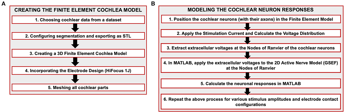
Figure 1. Illustration of the flow chart to construct the FE cochlear model. (A) Creating the finite element cochlea model. (B) Modeling the cochlear neuron responses.

FIGURE 2

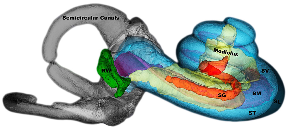
Figure 2. The selected dataset is shown as 3D image in ITK-SNAP. The structures are semicircular canals, modiolus, SG, spiral ganglion; BM, basilar membrane; SV, scala vestibuli; ST, scala tympani; SL, spiral ligament; RW, round window.

The size of each cochlear image was ~2.20 GB with more than a million voxels. To reduce computation time, we imported the STL files into Simpleware™ software (Version 2021; Synopsys, Inc., Mountain View, USA) and reduced the size of the mesh for certain computational tasks without sacrificing resolution in critical segments of the model. Then, we exported the parts as STL files. Geomagic (3D Systems, Morrisville, NC) and Hypermesh (Altair Engineering, Troy, MI) software tools were utilized to clear the noise, delete unwanted parts, and refine the mesh in the data (Figure 3).

FIGURE 3

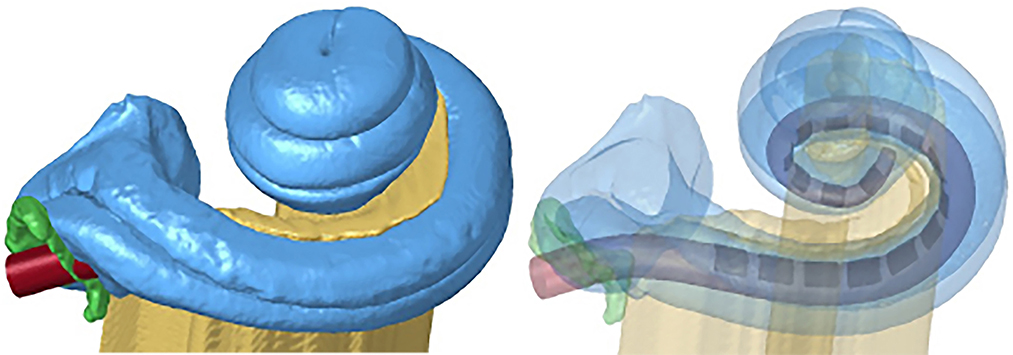
Figure 3. Finite element model of the cochlea and electrode array design (in red).

The model was completed by adding the electrode array inside the scala tympani. We used PTC Creo Software (PTC, Boston, MA) for the electrode design that consisted of 16 platinum contacts (conductivity σ = 2.5 × 10⁶ S/m) and a silicon carrier (σ = 10⁻¹² S/m) (Table 1). The electrode array geometry was based on the Advanced Bionics (Sonova, Valencia, CA, USA) HiFocus 1J commercial lead and positioned laterally closer to the modiolus inside the scala tympani.

TABLE 1

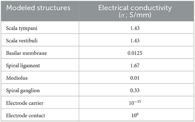
Table 1. Electrical conductivity for various compartments of the cochlea (Strelioff, 1973; Spelman et al., 1982; Finley et al., 1990; Frijns et al., 1996; Hanekom, 2001; Rattay et al., 2001a; Hanekom and Hanekom, 2016).

The length of the basilar membrane in our human data was ~23 mm and the total length of the electrode was ~17 mm. Finally, this model was pre-processed to construct a 3D model using Synopsys' Simpleware™ FE module and then a volumetric mesh was generated consisting of 20,528,625 tetrahedra elements.

2.2. Electric potential distribution inside the cochlea

A finite element model (FEM) of the cochlea was developed in COMSOL Multiphysics 5.4a^® (COMSOL AB, Stockholm, Sweden). Electric potentials inside the cochlea induced by a current applied to each one of the electrode contacts were simulated by applying the Poisson's equation (Eq. 1) at each finite element of the model mesh as a volume conductor using COMSOL AC/DC Module.

$\begin{array}{ll}{\nabla }^2\phi =-\frac{I_s}{\sigma }& (1)\end{array}$

where φ is the electrical potential, I_s is the current source, and σ is the specific conductivity.

Four different electrode contact configurations were tested to investigate the effect on stimulation selectivity:

i. Monopolar (MP): cathodic current is applied to one electrode contact and the outer boundaries of the volume conductor were grounded for the return current.

ii. Bipolar (BP): two currents with the same amplitude and opposite polarities are applied to adjacent contacts.

iii. Tripolar (TP): cathodic current is applied to the center contact and the anodic current is divided into two equal parts and applied to the adjacent two contacts on each side of the cathode.

iv. Distant Bipolar (DB): cathodic current is applied to one contact, and the anodic current to any of the remaining contacts to steer the extracellular field. The anodic electrode that generated the best results was searched for each cathode.

A monophasic rectangular current pulse with 0.2 ms duration is used in all electrode configurations, although a biphasic charge-balanced current waveform is typically used in cochlear stimulators. The monophasic waveform was chosen for simplicity since the sole purpose of the preceding phase in the biphasic waveform here would be to reverse the charge injected in the main phase and thus prevent drifting of the electrode voltage. The effect of the preceding phase is negligible if there is sufficient time gap between the two phases (Gorman and Mortimer, 1983), as we confirmed in our simulations. The stimulus current pulse was simulated by scaling the extracellular voltage amplitudes generated in COMSOL for a unit current.

2.3. Situating the cochlear neurons in the extracellular voltage field

To predict the electrical behavior of individual auditory nerve fibers, the electrical potentials at all mesh points of the cochlear model were extracted in COMSOL (scatteredInterpolant function for linear interpolation) and imported into Matlab (The Mathworks, Inc., Natick, MA, USA). Since the nerve fibers are not visible in the micro-CT images, a priori knowledge of the morphology of the fibers was used to estimate their position and trajectory.

We assume that the unmyelinated terminal of the fibers is positioned at the middle point of the basilar membrane between the scala tympani and scala vestibuli, and leave out the micro scale details of the connections to the hair cells for model simplicity (Figure 4—number one). We believe this simplification did not affect the results significantly since the activation never took place at the fiber tip. The fiber proceeds into the modiolus and then posteriorly to the spiral ganglion where the cell soma is located adjacent to the scala tympani within the modiolus (Figure 4—number two). The fiber continues radially outward from the modiolus into the internal auditory canal (IAC) where the auditory nerve is formed (Figure 4—number three) by the cumulation of fibers and projects to the auditory cortex. The trajectory of the fiber connecting the unmyelinated terminal to the soma and then to the IAC endpoint that matches the anatomical shape of the cochlea was formed using these three locations marked by three circles in Figure 4. Matlab's csaps function is used for creating three cubic splines passing through the three coordinates. Then, cscvn function is applied for smoothing and interpolating three cubic spline curves (Figure 5A). Finally, the x, y, and z coordinates of all the fibers along 2.5 turns of the cochlea are extracted from Hypermesh and then imported into Matlab.

FIGURE 4

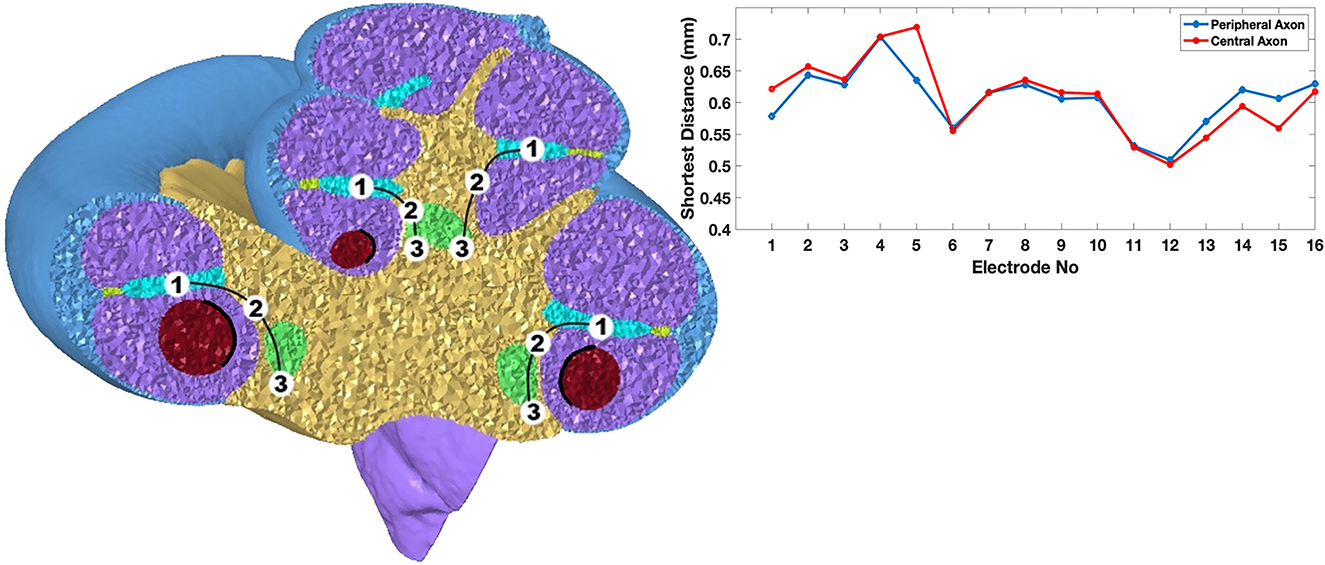
Figure 4. (Left) A cross-sectional view of the cochlea where the scala tympani (purple), modiolus (yellow), basilar membrane (cyan), spiral ganglion (green) and silicone electrode carrier (red) are shown. The locations marked are: 1. the middle point of the basilar membrane, 2. the cell soma in the spiral ganglion, and 3. a point of passage for the proximal fiber where the cochlear nerve is formed. (Right) Shortest distances from the center of the electrode contacts to the nearest cochlear fiber. The electrode distance to the closest node of Ranvier in the central and peripheral axons of the nearest cochlear fibers are plotted.

FIGURE 5

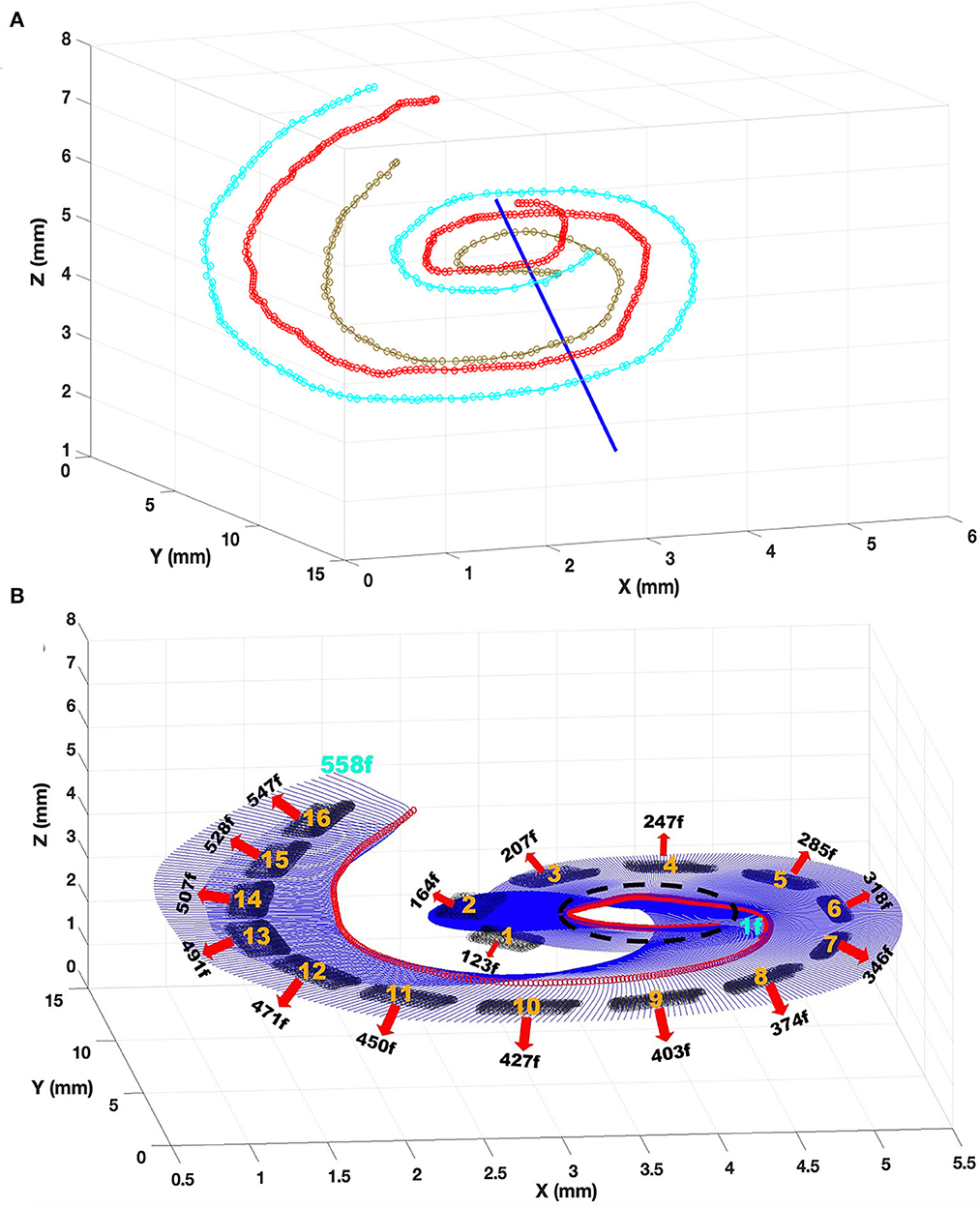
Figure 5. Steps of the procedures to create cochlear nerve fibers. (A) Interpolated trajectories using three cubic splines are created through three nerve components marked: 1. the middle point of the basilar membrane (cyan), 2. the cell soma (red), and 3. a point of passage for the proximal fiber in the spiral ganglion (light brown). The blue line shows the central axis of the cochlea. (B) Estimated trajectory of 558 auditory nerve fibers (blue) and the somas (red circles), and the electrode contacts (black shading). The fiber numbers nearest to the center of the electrodes are marked down.

To connect three splines and then create fiber trajectories, a center reference point is needed. The center point from the top view and the bottom view of the cochlea are marked in HyperMesh. These two points are extracted from HyperMesh and then imported into Matlab. A line is created connecting these two points to form a central axis for the cochlea (linear line in Figure 5A). This central line is used as a reference for calculating the radial angles at all points on the three spirals starting from the initial point of the basilar membrane. The points along the three spirals were calculated that are 1° apart as the center line being the apex of the angle. Finally, csaps function is used again for creating a cubic spline passing through each set of three points marked on the spirals to form the trajectory of a total of 558 nerve fibers corresponding to one and a half turn of the cochlear spiral (Figure 5B), similar to a previous study (Kalkman et al., 2014). Also, the positions for the 20 nodes of Ranvier are created on each fiber according to the spacing shown in Figure 6. These node of Ranvier coordinates did not fall on the node of the FE mesh (Potrusil et al., 2020). The extracellular voltages at the exact nodal positions were computed by interpolating the voltages at the neighboring nodes of the mesh.

FIGURE 6

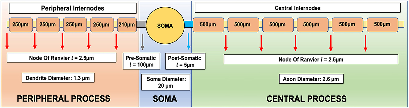
Figure 6. Compartmentalized model of an auditory nerve including the peripheral (distal) and proximal fibers, which are myelinated, and the soma. Geometric parameters are adopted from Potrusil et al. (2020).

2.4. Compartmental active nerve model in Matlab

A human auditory nerve fiber consists of a peripheral axon, the pre-somatic region, the soma, and the central axon (Figure 6). A compartmental nerve model incorporating the active and passive membrane properties was developed in Matlab, with geometric parameters adopted from Potrusil et al. (2020), to determine the activation threshold for each one of the auditory nerve fibers. The electric potential field generated varies along the spiral of the cochlea and results in a different response in each nerve fiber. The extracellular electric potentials at the assumed positions of the nodes of Ranvier are transferred from the COMSOL environment to Matlab as an input to the nerve fiber model in order to predict the threshold current for each fiber and at which node the action potential is initiated (Frijns et al., 1995; Hanekom, 2001, 2005).

For the active behavior of the nerve membrane in the unmyelinated parts, we used the generalized Schwarz-Eikhof-Frijns (GSEF) auditory nerve fiber model (Frijns et al., 1995). The GSEF model, which is based on Frankenhaeuser–Huxley (FH) (Frankenhaeuser and Huxley, 1964), explains the membrane kinetics of the myelinated nerve fiber in the frog. Frijns (1995) modified the FH model for the guinea pig cochlea. They assumed uniform finite-length fibers for all neurons in the cochlea. The equation consists of three time-independent matrices A, B, and C (Eq. 2). A and B are tridiagonal matrices that calculate the resistive coupling between compartments and C is a diagonal matrix containing the nodal capacitances.

$\begin{array}{ll}\frac{dV}{dt}=AV+Bd{V}_e+C\left[I_{Na}+I_K+I_L\right]& (2)\end{array}$

V_e represents the extracellular voltages due to the stimulating electrode and V represents the deviation from the resting membrane potential at each node as a function of time to determine if a propagating action potential is generated on the nerve fiber. I_Na is the sodium current, I_K is the potassium current, and I_L is the leakage current.

To calculate the nerve fiber responses, extracellular voltages exported from COMSOL were applied as external excitation potentials at the nodes of Ranvier in each nerve fiber. Then, the threshold currents at each node were determined for the occurrence of an action potential by iteratively changing the stimulus current intensity, which is implemented by scaling the extracellular voltage field generated for a unit current in the FEM. Threshold currents for MP, BP, TP, and DB electrode configurations are computed for all fibers. The nerve fiber is considered to be activated at the current level that stimulates at least one node. The lowest thresholds for all the nerve fibers are plotted to investigate the spatial change of threshold and thus the stimulation selectivity along the cochlear spiral.

3. Results

3.1. Potential distributions in the cochlea

The voltages measured at the nodes of Ranvier of all the cochlear neurons are plotted for four different electrode configurations (MP, BP, TP, and DB) in Figure 7 (top panel) where contact 5 served as a cathode in all cases for comparison. MP field has a wider spread across the fibers than all other configurations and does not switch polarity along the initial 20 nodes depicted. The peripheral nodes distal to the soma, the soma, and the central nodes close to the soma are exposed to the most negative extracellular voltages inside the basilar membrane.

FIGURE 7

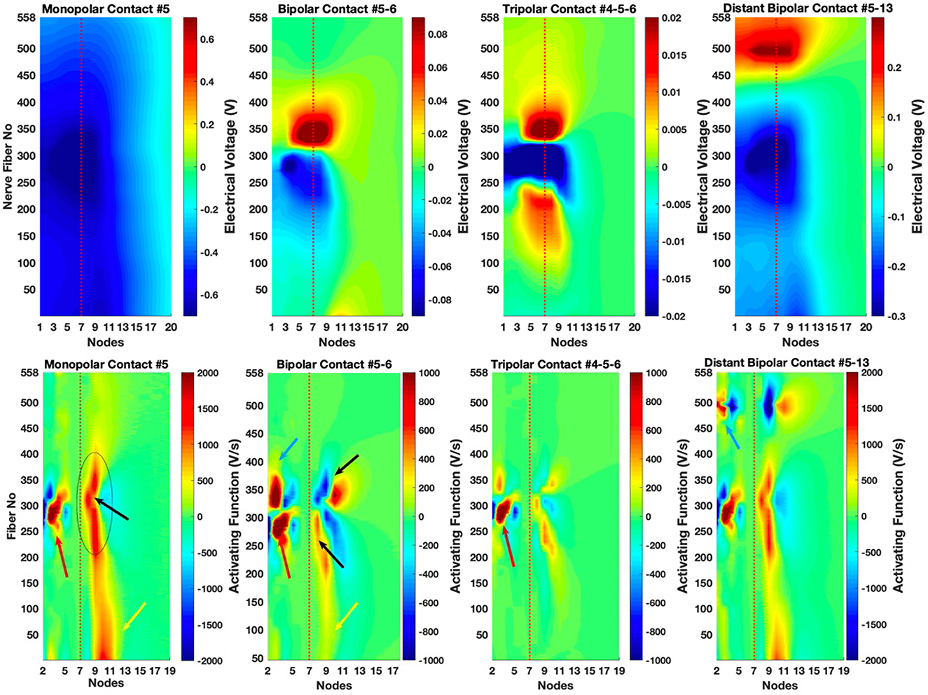
Figure 7. Extracellular voltages and activating function as a function of the node and fiber numbers. (Top panel) Extracellular voltage profiles, measured at the nodes of Ranvier, are plotted for all configurations in which contact 5 is the cathode for comparison. (Bottom panel) The activating function calculated according to Eq. 3 along each fiber. Node 7 corresponds to the soma (red dash lines).

For the BP, the contact 6 serves as the current return electrode (anode). The BP field has much sharper peaks around the contacts and quickly decreases to zero at the central nodes, but the most negative voltages are about eight times smaller than that of the MP.

For the TP, the contacts 4 and 6, flanking contact 5, serve as the anodic contacts with equal share of the return current. The TP configuration generates even a sharper voltage field by limiting the spread of the current on both sides of the cathodic contact. The negative peak (−0.07 V, out of the chosen range in Figure 7) is slightly smaller than the BP peak (−0.09 V). More importantly, in both BP and TP configurations, the spatial extent of the negative field is much shorter than that of the MP across the fibers, i.e., along the basilar membrane.

For the DB, contact 13 (near fibers 485–495) serves as the anode in order to steer the current in a direction orthogonal to the basilar membrane. The DB field represents a midway solution between MP and BP configurations in terms of the voltage spread and the peak amplitudes. The cathodic voltage spreads less and the negative extreme of the voltages are smaller than the MP field (−0.27 V vs. −0.7 V).

3.2. Activating function

Activating function (AF, Eq. 3), proposed by Rattay (1986, 1999) and quantifies the rate of increase in the membrane potential at the start of the stimulus pulse, is a reliable predictor of where the action potential is initiated along then axon, although small deviations may occur in this prediction for long pulse durations (Warman et al., 1992). The positive values in Figure 7 (bottom panel) indicate depolarization of the nodal membrane, and vice versa.

$\begin{array}{ll}ActivatingFunction(AF)=\frac{\left[\frac{V_{e,n-1}-V_{e,n}}{\frac{R_{n-1}}{2}+\frac{R_n}{2}}+\frac{V_{e,n+1}-V_{e,n}}{\frac{R_{n+1}}{2}+\frac{R_n}{2}}\right]}{C_{m,n}}& (3)\end{array}$

where n is the node number, R_n is the axoplasmic resistance at node n to the neighboring nodes, and C_{m, n} is the membrane capacitance at node n.

Nearest to Contact 5 are the fibers 260 through 285. There is a positive peak at the third nodes of the fibers between 270 and 300 in the MP plot (red arrow, Figure 7, bottom panel). In agreement to this, the lowest stimulation thresholds occur at those fibers according to the simulations of the active axon model in Matlab (Figure 9, top panel). The AF plot (MP in Figure 7, bottom panel) also suggests that the fibers from 200 to 400 are depolarized at the central nodes of 8 and 9 (black oval). This is mostly due to the anatomical features of the cochlea that nodes 8 and 9 happen to be where the cochlear fiber has a curvature yielding a larger second difference. The threshold and node plots in Figure 10 also agree with this prediction. Finally, positive values in the AF predicts low thresholds at node 10 of fibers 1–50 (yellow arrow), as also confirmed by the threshold plot. This low threshold region occurs, however, for a completely different reason. The cochlea spirals inwardly, first moving away from contact 5 and then making a turn and starting to come back toward contact 5 (dash oval in Figure 5B). Thus, the fibers with the smallest numbers on the inner turn of the cochlear spiral tend to have low thresholds because of their proximity to contact 5. A similar phenomenon occurs for all the contacts from 3 through 7 (except 5) where some of the fibers within the 1–100 range present even lower threshold than the ones nearest to the cathode due to spiraling of the cochlea.

In the AF plot for the BP stimulation, there is a dark red island between the fibers 270 and 300 in Figure 7 (bottom panel), as in the MP plot, for the most distal nodes (red arrow). The second most strong values of the AF function occur for the fibers 325–375, also at the distal nodes, nodes 2–3 (blue arrow) and around the central node 10. This is surprising since the anodic contact (near fibers 300–325) is very close to those fibers. However, the AF peaks on each side of the anodic contact due to the second difference of the voltage along the fibers and gives rise to low threshold regions. There is a low threshold area at the lower end of the fibers (1–50) as in the MP plot (yellow arrow), but the effect is much weaker due to containment of the electric field into a smaller area with the BP configuration. The two red islands in the AF at the central nodes of the fibers within the 200–350 range (black arrows) are not strong enough to impose lower thresholds than those at the proximal nodes of the same fibers. But these peaks tend to widen the threshold plots (see the discussion on the side lobes) because of their wider spread across the fibers.

The AF plot for the TP predicts a focal point at the peripheral nodes of the fibers between 270 and 300 as in MP and BP (red arrow). The fiber curvature effects are small enough that they do not produce other significant local maxima in the activating function. As seen in Figure 9, the threshold plot for the shown amplitude range is contained in a much narrower fiber range compared to the other configurations.

DB activating function is very similar to that of MP around the cathodic contact and at the fibers 1–50, although the secondary peaks are weaker. The anodic contact (number 13) generates additional low threshold areas at the most distal nodes (node 3) of the fiber numbers around 500 (blue arrow), but fortunately not as strong as those near the cathode.

3.3. Current threshold vs. fiber number

Threshold currents are computed using the compartmental nerve model in Matlab based on the extracellular nodal voltages found from the FE model. Regarding the distant bipolar (DB), the region of neural excitation near the cathode can be shaped gradually by carefully selecting the electrode for the return current, i.e., by current steering. We took a closer look at how the threshold curve changes when the return current (anode) is applied through different contacts for current steering and compared them with the other three configurations (Figure 8). The threshold curve for DB using contacts 5 and 10 resembles the MP curve (black and red respectively) and thus does not provide lower thresholds or better spatial selectivity over MP. As the return current is switched to contacts 5 and 3, the curves (dash lines) start resembling that of BP (green) and TP (blue) in terms of the horizontal spread. But the minimum threshold currents stay at the low values similar to MP (around fiber 282). This suggests that the placement of the anodic contact can steer the field in a way to reduce the spread of the current along the basilar membrane without increasing the thresholds at the center of the targeted group of fibers.

FIGURE 8

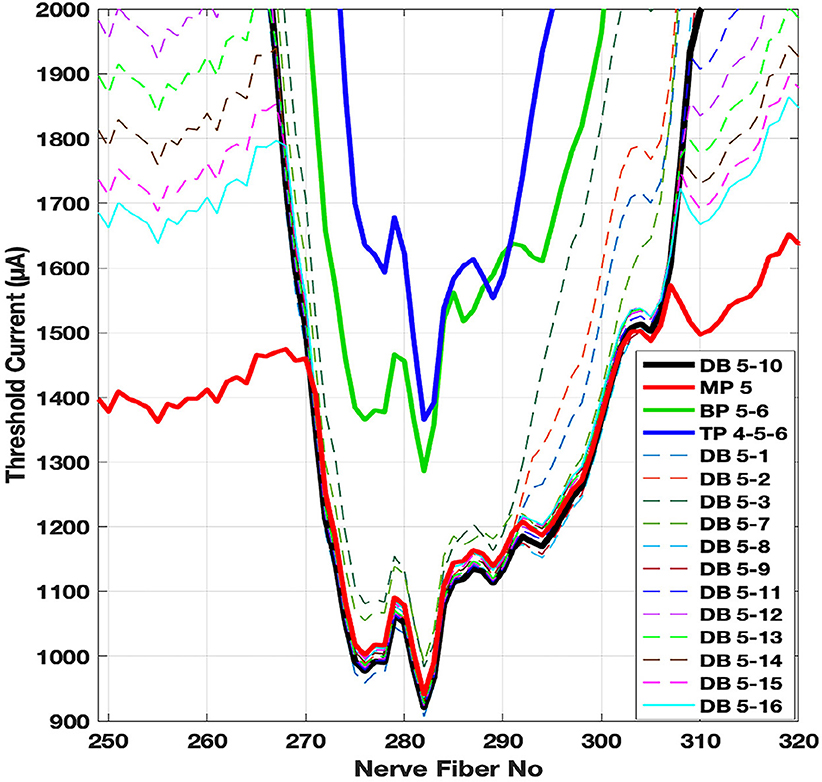
Figure 8. Threshold curves for DB stimulation, where the return current (anode) is applied at selected contacts from 1 through 16, is compared with other electrode configurations. A narrow range of fibers are selected on the horizontal axis for better visualization. MP (contact 5): red, TP (contacts 4-5-6): blue, BP (contacts 5 and 6): green, DB (contacts 5 and 10): black, and DB (other contact combinations): dash lines.

Minimum currents required to generate an action potential and the node at which it is initiated are plotted for all the fibers in Figure 9 for the extracellular nodal voltages shown in Figure 7. In general, the action potential initiation point was at nodes 2–3 on the peripheral axon for the fibers with the lowest threshold points. The threshold was higher for the fibers that are further away from the cathodic electrode and the node of action potential initiation moved more proximally and jumped to the central nodes (nodes > 7). The unexpected finding was that the threshold curves had lobes of local minima on each side of the main lobe, which sometimes had even lower thresholds. These side lobes are a result of stimulations switching from peripheral to the central nodes due to the curved trajectory of the nerve fibers in this voltage field. However, these side lobes are not due to jumping of the stimulus point to opposite side of the spiral as seen with MP having low thresholds at fibers 1–100. These secondary low-threshold regions are an undesired side effects since they will compromise the spatial selectivity of the stimulation.

FIGURE 9

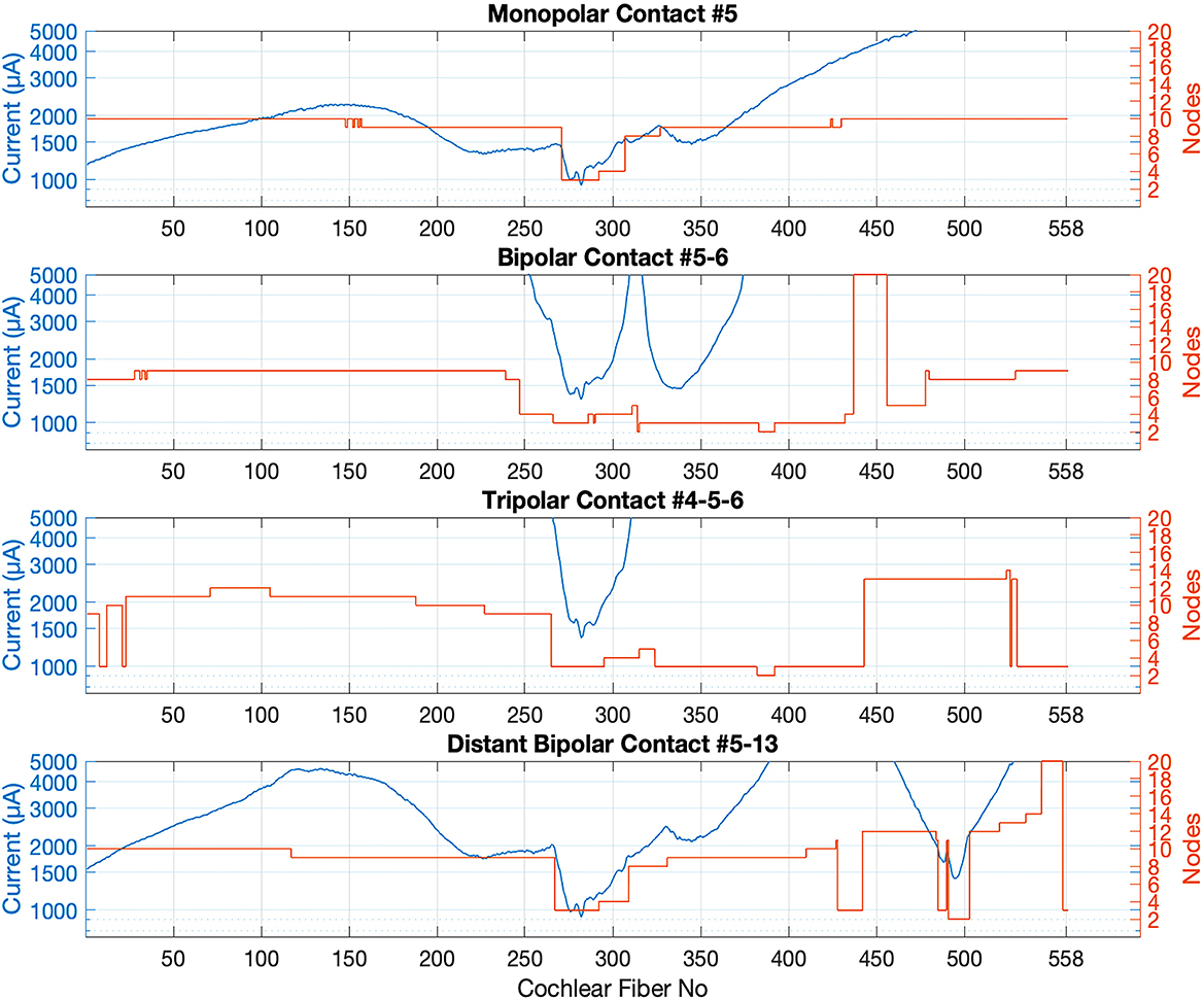
Figure 9. Threshold current profiles for all electrode configurations in which contact 5 is the cathode. The red plots indicate the nodes of Ranvier where action potential is initiated in each cochlear neuron. Node 7 represents the soma.

MP and DB configurations have the lowest thresholds (941 μA and 979 μA) on the fibers near contact 5 (node 281) because they produce the largest voltage fields. The BP and TP stimulations have higher thresholds, but narrower spread of excitation across the fibers than the MP stimulation. TP has the highest thresholds (1,365 μA at node 281) of all.

The threshold currents and the nodes at which the action potential was initiated are shown for all electrodes in Figure 10. For DB, the anodic electrode that produced the largest Threshold Margin (see below for definition) was found for each cathodic electrode individually (Table 2). Threshold currents vary depending on the contact number, however, the relative amplitudes for different configurations follow the general trend presented specifically for contact 5 in Figure 9. TP and BP have higher thresholds than MP and DB configurations in all cases. In contacts 7–9, the threshold is slightly higher for BP than it is for TP, but they are comparable in most cases. The DB and MP thresholds are also very similar in all cases. Action potential is initiated mostly at the peripheral nodes 3 through 5, but in some cases jumped to the central nodes 8 or 9. This happened in seven electrodes with MP, five electrodes with DB, four electrodes with TP, and three with BP. Stimulation jumped to the central axon with MP and DB in every case where BP and/or TP did the same. Soma is never the lowest threshold point (node 7), possibly due to its high membrane capacitance and small transmembrane resistance.

FIGURE 10

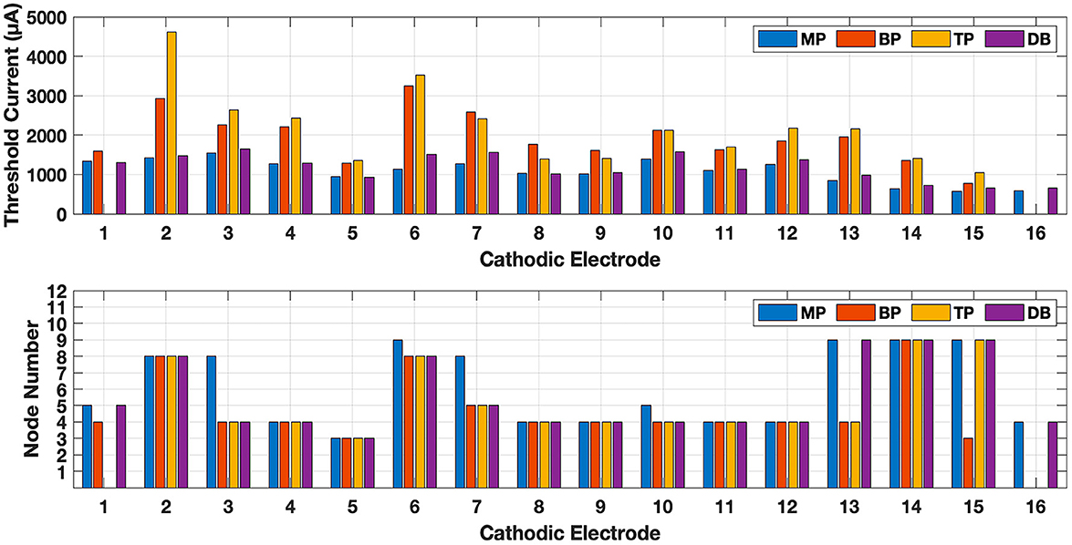
Figure 10. Threshold currents (top panel) and the nodes of Ranvier (bottom panel) at which the action potential is initiated for all electrodes of the array and for monopolar (MP), bipolar (BP), tripolar (TP) and distant bipolar (DB) electrode configurations. Note that x-axis shows the cathodic electrode number in each case. TP configuration is not possible when electrode 1 or 16 is the cathode for the lack of flanking anodic electrodes. BP also does not exist for the 16th electrode for the same reason.

TABLE 2

Table 2. Optimum cathode-anode combinations for the DB stimulation.

Finally, we investigated how much would the exclusion of the electrode carrier make in the activation thresholds by removing it from the model while keeping the electrode contacts in place, as also questioned by Potrusil et al. (2020). As an example, the thresholds for the electrode 5 increased by 36%, 44%, 67%, and 36% for MP, BP, TP, and DB configurations, respectively, in the absence of the electrode carrier, although the overall shape of the threshold plots (as in Figure 9) did not change noticeably. Thus, the threshold currents were substantially higher in all cases with no carrier in place and it should be included in the model for accuracy of the predictions.

3.4. Threshold margins

The focality of stimulation determines how many independent channels of stimulation can be achieved with cochlear implants. The spatial extend of the activation before the stimulation point jumps or spills over a distant fiber can be defined as Threshold Margin (ThresMar). In our model, there are 16 contacts spanning 558 fibers of the cochlea. Ideally, we would expect each contact to stimulate ~35 fibers on average, not more and not less, in order to uniformly cover all the fibers with 16 contacts. We could then define ThresMar to quantify how successfully an average of 35 fibers per electrode can be achieved as follows: the threshold current is gradually increased at the cathode until at least 35 consecutive fibers are stimulated near the cathode (Figure 11). If a horizontal line (red line) drawn at that current level intersects the threshold curve anywhere else outside the stimulated 35 fibers, those fibers (the second lobe on the right) would be activated by this current as well. The minimum threshold point for this second set of fibers is found and divided by the minimum of the primary set and expressed as a percentage (Eq. 4).

$\begin{array}{l}ThresholdMargin(ThresMar)\\ =(\frac{MinimumThreshol{d}_{centralfiber}}{MinumumThreshol{d}_{elsewhere}}-1)\times 100& (4)\end{array}$

FIGURE 11

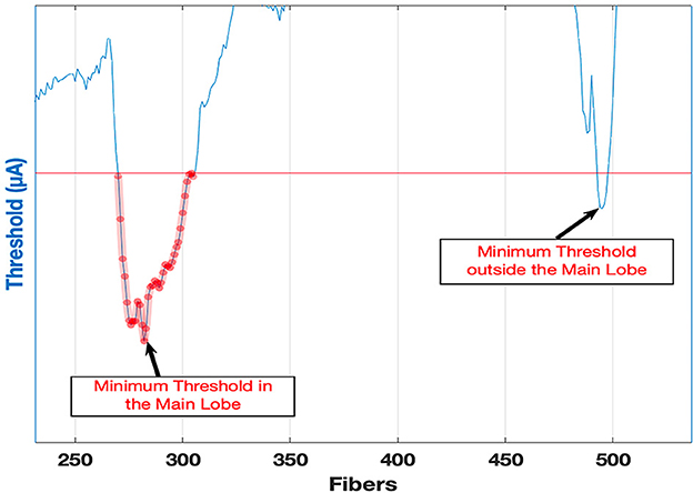
Figure 11. The method of calculating the Threshold Margin for an electrode based on the current threshold curve. Example is for TP contacts 7-8-9.

This metric quantifies how much the current can be increased before the activation jumps outside the targeted zone of fibers while the total number of fibers in the targeted zone does not exceed a maximum number of 35 for each electrode. For instance, 100% implies that the current can be doubled without off target activation and without stimulation of more than 35 fibers in the targeted zone. A 0% or a negative value indicates that the stimulation jumps to another part of the basilar membrane before even a single fiber is activated in the targeted zone. In Figure 12, if the red line did not cross the threshold plot anywhere else, the threshold value at the edge of the 35 consecutive fiber block would be taken and divided by the minimum to find ThresMar.

FIGURE 12

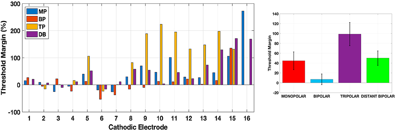
Figure 12. Threshold margins for all electrode configurations according to Eq. 4. The bar plot on the (right) shows the average and ±standard error for each type.

ThresMars (Figure 12) show that TP presents the largest percent margins especially in the outer electrodes (>7), followed by MP and DB. BP has the smallest margins in general except in electrode 15. The ThresMars are very low or even negative for most of the configurations with electrodes (cathodic) 1 through 7 where the side lobes tend have a smaller threshold than the main lobe near the cathodic electrode, due to activation at the central nodes. The mean ±standard error for MP, BP, TP, and DB are 44.7 ± 18.1, 7.68 ± 10.9, 98.8 ± 23.6, 50.1 ± 14.7 percent, respectively. On average, DB increased the ThresMars slightly over MP, but TP had the highest margins. BP was the lowest.

3.5. Average number of fibers per electrode

An additional piece of information that can be presented here is the actual number of fibers that are stimulated per electrode before the current jumps outside the targeted zone. In a perfect scenario, the number of fibers for all electrodes would be 35. Any value <35 at any electrode would imply that some of the 558 fibers will not be accessed when the maximum number of fibers at the other electrodes is limited to 35 in order to keep the stimulation focal.

The maximum number of fibers stimulated without spillover is shown Figure 13. The mean ±standard error for MP, BP, TP, and DB are 23.2 ± 3.6, 10.0 ± 3.4, 19.3 ± 3.6, 20 ± 3 fibers respectively (bar plot in Figure 13). A one-way ANOVA confirmed a significant effect of electrode configurations [F_{(3, 57)} = 2.846, p = 0.0455]. Post-hoc independent-samples t-tests, using a Bonferroni correction (alpha adjusted to 0.0125), revealed significant differences between MP and BP only [t₍₂₉₎ = −2.66, p < 0.0125]. Electrode 6 is the worst-case scenario where the stimulation jumps to a distant location before even one fiber can be stimulated at the targeted range of fibers for all configurations. This is because electrode 6 is the nearest to the fibers 1–100 (Figure 5B) and those fibers are activated first before the targeted fibers 300–325.

FIGURE 13

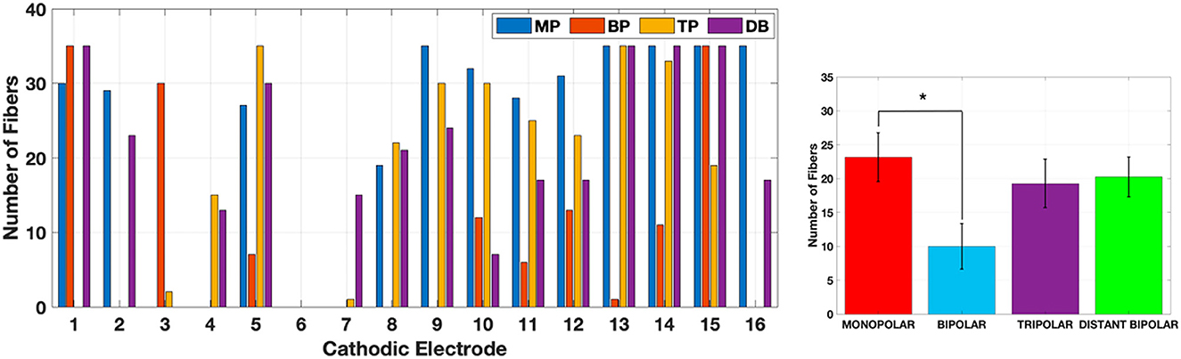
Figure 13. Number of fibers stimulated in each electrode configuration before spillover. The bar plot shows the average and ±standard error for each type. ^*Only MP mean is statistically different than BP (ANOVA, alpha adjusted to 0.0125).

Although the average across all electrodes do not favor DB over MP or TP, when individual cases were compared, in fact the DB improved ThresMars in nine electrodes out of 16, and increased the number of fibers stimulated in 5 of those 9. The ThresMars was 31% ± 8.5% (mean ± SE, range 6%−84%) higher with DB over that of MP in those nine electrodes and 3.8 ± 1.8 (mean ± SE, range 0–15 fibers) more fibers were stimulated per electrodes by those same nine electrodes.

4. Discussion

Our main objective in this study was to revisit the multipolar stimulation methods in a computational model that incorporated a realistic cochlear gross anatomy with complex inner ear geometry that is extracted from human μ-CT images, and that which included a commercial stimulation lead design. We also introduced a novel stimulation paradigm (distant bipolar) for current steering.

4.1. The AF patterns

The AF patterns around the cathodic electrodes appeared to be very similar regardless of the electrode configuration (Figure 7, bottom row), suggesting minimal interaction from the anodic contacts. Interference between the contacts can increase with larger separations between the basilar membrane and the electrode carrier in the scala tympani (Frijns et al., 1996, 2001; Hanekom, 2001; Briaire and Frijns, 2006; Seeber and Bruce, 2016). The additional AF peaks that emerged for the anodic electrodes in the BP and DB configurations were much weaker in the case of TP. The interesting, and perhaps unexpected observation was that each electrode had two positive peaks (depolarization) in the AF plots, one at the peripheral and the other at the central nodes, and usually two negative peaks (hyperpolarization) adjacent to the positive peaks. The AF along a straight myelinated axon in a homogeneous medium predicts two hyperpolarized lobes on each side that are four times weaker than the depolarization peak near the cathode in the center (Ranck Jr, 1975; Rattay, 1986, 1987, 1989) This agrees with the AF patterns due to the cathodic contact alone at the peripheral nodes. The additional depolarized and hyperpolarized points emerging at the central nodes seem to be related to the unique geometry of the cochlear neuron with its curved shape and the presence of the soma in the center. The electrode contacts were almost at equidistance from the peripheral and central axons of the nerve positioned inside scala tympani (Figure 4). The relative strengths of depolarizations at the peripheral and central axons would change depending on how the electrode carrier is positioned inside the scala tympani.

The fibers in the ~1–50 range presented low current thresholds with electrodes 5 through 9 of the MP configurations, due to spreading of the voltage field to the apex, and the first activated nodes were the central nodes 10 and 11. This limited the ThresMar and lowered the average number of fibers per electrode before the current jumps to the apical fibers. This issue does not appear to be present in the plots of Kalkman et al. (2015) which could be due to differences in the assumed spatial distributions and the trajectory of the auditory nerve fibers in the two models. The TP had larger current margins with the electrodes located in the outer spiral of the cochlea. However, BP suffered from stimulation spillover to adjacent fibers due to virtual peaks created in the AF by the anodic contact (Figures 9, 11). The DB method introduced in this study searches for an optimum choice for the anodic electrode in order to steer the current and overcome the disadvantages of the MP an BP methods. The DB provided a larger ThresMar than MP in most of the electrodes, while having comparable stimulation thresholds (Figure 10). Thus, the DB technique can be applied selectively to individual contacts whenever there is potential for improving threshold margins and thereby selectivity.

4.2. Stimulation threshold plots

The excitation took place mostly in the peripheral axon, though not always near the end (Rubinstein, 1993; Rattay, 2008; Rattay et al., 2017) and jumped to the central axons in a few electrodes (Figure 10, bottom row). Selectivity with focal stimulation was achieved and was better in the outer turn of the cochlear spiral, with all configurations without resorting to the use of simultaneous pulses for leveraging field interactions. This is in contrast to the findings of Kalkman et al. (2015) which suggested that selective stimulation is only possible if the excitation occurs in the central axon when the focal electric fields are able to penetrate into the spiral ganglion. The discrepancy in our results may be because we adopted the compartmental neural model developed by Potrusil et al. (2020) where the peripheral axon is longer, although the neural membrane dynamics were based on the model developed by Frijns et al. (1994, 1995, 1996). The relative distance of the electrode contacts to the central and peripheral axons plays a significant role on the focality of the stimulation and the initiation point of the action potential (Litvak et al., 2007; Smit et al., 2008; Frijns et al., 2009; Goldwyn et al., 2010; Seeber and Bruce, 2016). The shortest distance from the electrode centers to the central and peripheral axons of the closest fibers were approximately the same along the entire electrode lead in our model (Figure 4), and thus cannot be the reason behind initiation of activation preferably in the peripheral axon. The endings of the fibers had an unmyelinated terminal for 10 μm as in Potrusil et al. (2020), and those near the cathode were hyperpolarized as seen in the AF plots in Figure 7.

Almost all plots of the threshold current as a function of the fiber number contained lobes on each side of the main lobe near the cathode (Figure 9). These side lobes were not due to stimulation point jumping to distant fibers, or because of the electric fields generated by the anodic contacts as suggested by Kalkman et al. (2016) but because of the central nodes having thresholds slightly above that of the peripheral axons. This is clearly shown in the AF plots in Figure 7 where the red regions at the central nodes (8–10) span a much wide fiber range than the ones in the peripheral nodes. This must be because of the fact that the central axons draw closer to each other as they travel down the modiolus. As a result, the electric field of a similar spatial extent affects a large number of central axons in the modiolus than the peripheral axons in the basilar membrane. Phased arrays were suggested as a potential solution to eliminate these side lobes (Frijns et al., 2011). The DB method proposed here also weakens the side lobes by reducing the AF peaks at the central nodes (Figure 7) and increases the ThresMar. Note that the improvements in selectivity suggested by the results of the present study can be combined with other methods that can achieve focal stimulation (e.g., simultaneous multi-contact stimulation or using different temporal waveforms) since the electric fields in volume conductors scale linearly and they are additive.

The threshold differences between the peripheral and central axons are smaller for the electrodes in the apex, probably because the central axons are even more closely packed than they are in the outer spiral of the cochlea. As a result, the ThresMars are very small or negative for the first seven electrodes regardless of the configuration (Figure 12) in agreement with Bai et al. (2019). In order to achieve selective stimulation and larger current margins in the apex, the electrodes should be made smaller and positioned with smaller spacing in between and perhaps closer to the basilar membrane inside scala tympani.

4.3. Model validation

Despite the lack of electrophysiological data to validate our results, the insight that can be gained through modeling can be valuable. The AF closely agreed with the fibers of lowest threshold predicted by the active compartmental model, and it was useful to gain insight for the mechanisms underlying the stimulation profiles with multipolar electrode configurations and a novel method, the distant bipolar method. Our nerve model adopted from Potrusil et al. (2020) contained 20 nodes including the soma. The simulations were run with lower number of compartments, by removing the five most proximal ones, in order to check if the number of compartments were sufficient for the accuracy of threshold predictions. The threshold currents were <5% different with the shorter model indicating that adding more compartments would not change the results significantly. We also checked if the boundary conditions would introduce significant changes in the results. We made the surrounding box around the cochlea smaller (50 mm × 50 mm × 50 mm) than the current size (100 mm × 100 mm × 100 mm), which altered the extracellular voltages again <5%. The mesh size inside the cochlea was the smallest available in COMSOL and much smaller than the spatial extent of any local variations seen in the voltage fields.

4.4. Isotropic conductivity

Reported cochlear implant models typically use isotropic conductivities for various compartments of the cochlea. This may be sufficient for most cochlear inner structures. But the electrical currents cannot be conducted equally well in all directions in the modiolus because the auditory nerve fibers introduce a great deal of anisotropy and take up a notable size of space. Adding anisotropy to the cochlea model to account for the presence of such structures could have a significant effect on the results and should be implemented in the future for more realistic results (Kalkman et al., 2016; Fellner et al., 2022). A detailed geometry for the human head could also be incorporated into the model to achieve more realistic distributions of the voltage field at the boundaries of the cochlea. Our experience, however, agrees with another report Potrusil et al. (2020) that the boundary conditions mostly add a common shift to the voltage and do not affect the AF profiles.

4.5. Trajectory of the auditory nerve fibers

In our model, auditory nerve fibers had an assumed smooth trajectory from the basilar membrane to the modiolus, a fixed length, and regular spacing, simply because the μ-CT images are not able to capture the trajectory of individual fibers. In the human cochlea, the fibers are bundled after passing the Organ of Corti through the basilar membrane (Cakir et al., 2019; Rattay and Tanzer, 2022). The actual trajectories of these fibers can vary considerably along the turns of the cochlea. Low threshold points will occur along these fibers whenever there is bending or an inhomogeneity in the extracellular conductivity at the micro scale, as suggested by Potrusil et al. (2020). In addition, other reports Frijns et al. (2015) and Badenhorst et al. (2016) found that adding stochasticity to the cochlear models plays a significant role in prediction of the stimulation thresholds. The present study was intended to provide a general understanding of how traditional multipolar stimulation results are affected by a realistic gross cochlear geometry and introduce the DB method, and therefore does not challenge the findings of other reports incorporating more sophisticated models of the auditory nerve anatomy and membrane physiology.

4.6. CT vs. μ-CT

In comparison to the size of the human cochlea and its internal structures, the resolution of contemporary clinical CT images is quite poor. As a result, images obtained from patients often lack information on the intracochlear anatomy and are therefore of limited use for the development of artificial hearing implants (Gerber et al., 2017). To compensate for the low resolution of clinical CT imaging, several attempts have been made to extract the desired geometric information (e.g., total cochlear duct length, position of the basilar membrane) from surrogate measurements made from CT images (Escudé et al., 2006; Erixon and Rask-Andersen, 2013). However, the intricacy of cochlear anatomy reduces the efficacy of these techniques. With the development of current imaging techniques such as micro computed tomography (μ-CT), the ability to gather comprehensive imaging information has enabled researchers to obtain previously inaccessible aspects of the cochlear structures (Teymouri et al., 2011). The reduced size of the scanning field of view and the high radiation dose necessary to attain a high degree of image quality are the current limits of this technology for clinical integration.

5. Conclusions

Overall, the results demonstrate once more that the stimulation patterns in a human cochlea may not be as uniform as predicted by idealized cochlear geometries used in some reported models (Rattay et al., 2001a). It is likely that each human cochlea will have slightly different anatomy and local inhomogeneities. Therefore, the optimum electrode configuration and the optimum set of current thresholds for each electrode will have to be determined in each subject individually. In the past, the traditional multipolar stimulation paradigms only considered adjacent placement of the electrodes or skipping one or two contacts in the bipolar configuration for current steering (Frijns et al., 1994, 1995, 1996; Heshmat et al., 2021). The optimum choice for the return current may be a distant electrode, as suggested by our results, in order to achieve larger current margins and thus selectivity. The commercial cochlear leads currently do not allow different electrode configurations most likely because of the limitations on the battery life. Complex electronics and current drivers that consume extra energy are required to implement such variations. Nonetheless, as the longevity of implantable batteries improves with technological advancements in that field and switch-mode electrode driving system that can also improve battery life are incorporated into the cochlear implants, these alternative stimulation paradigms should become available for the cochlear implant users in the near future.

Data availability statement

Publicly available datasets were analyzed in this study. This data can be found at: https://www.smir.ch/objects/204388.

Ethics statement

Ethical approval was not required for the study involving humans in accordance with the local legislation and institutional requirements. Written informed consent to participate in this study was not required from the participants or the participants' legal guardians/next of kin in accordance with the national legislation and the institutional requirements.

Author contributions

OC: Methodology, Software, Visualization, Writing—original draft. SP: Formal analysis, Methodology, Software, Supervision, Validation, Writing—review & editing. MS: Conceptualization, Formal analysis, Methodology, Supervision, Validation, Writing—review & editing.

Funding

The author(s) declare financial support was received for the research, authorship, and/or publication of this article. This work was supported by Faculty Seed grant from NJIT Research Office.

Conflict of interest

The authors declare that the research was conducted in the absence of any commercial or financial relationships that could be construed as a potential conflict of interest.

The author(s) declared that they were an editorial board member of Frontiers, at the time of submission. This had no impact on the peer review process and the final decision.

Publisher's note

All claims expressed in this article are solely those of the authors and do not necessarily represent those of their affiliated organizations, or those of the publisher, the editors and the reviewers. Any product that may be evaluated in this article, or claim that may be made by its manufacturer, is not guaranteed or endorsed by the publisher.

References

Badenhorst, W., Hanekom, T., and Hanekom, J. J. (2016). Development of a voltage-dependent current noise algorithm for conductance-based stochastic modelling of auditory nerve fibres. Biol. Cybern. 110, 403–416. doi: 10.1007/s00422-016-0694-6

PubMed Abstract | CrossRef Full Text | Google Scholar

Bai, S., Encke, J., Obando-Leitón, M., Weiß, R., Schäfer, F., Eberharter, J., et al. (2019). Electrical stimulation in the human cochlea: a computational study based on high-resolution micro-CT scans. Front. Neurosci. 13, 1312. doi: 10.3389/fnins.2019.01312

PubMed Abstract | CrossRef Full Text | Google Scholar

Bonham, B. H., and Litvak, L. M. (2008). Current focusing and steering: modeling, physiology, and psychophysics. Hear. Res. 242, 141–153. doi: 10.1016/j.heares.2008.03.006

PubMed Abstract | CrossRef Full Text | Google Scholar

Braun, K., Böhnke, F., and Stark, T. (2012). Three-dimensional representation of the human cochlea using micro-computed tomography data: presenting an anatomical model for further numerical calculations. Acta Otolaryngol. 132, 603–613. doi: 10.3109/00016489.2011.653670

PubMed Abstract | CrossRef Full Text | Google Scholar

Briaire, J. J., and Frijns, J. H. (2000). Field patterns in a 3D tapered spiral model of the electrically stimulated cochlea. Hear. Res. 148, 18–30. doi: 10.1016/S0378-5955(00)00104-0

PubMed Abstract | CrossRef Full Text | Google Scholar

Briaire, J. J., and Frijns, J. H. (2005). Unraveling the electrically evoked compound action potential. Hear. Res. 205, 143–156. doi: 10.1016/j.heares.2005.03.020

PubMed Abstract | CrossRef Full Text | Google Scholar

Briaire, J. J., and Frijns, J. H. (2006). The consequences of neural degeneration regarding optimal cochlear implant position in scala tympani: a model approach. Hear. Res. 214, 17–27. doi: 10.1016/j.heares.2006.01.015

PubMed Abstract | CrossRef Full Text | Google Scholar

Cakir, A., Labadie, R. F., and Noble, J. H. (2019). “Auditory nerve fiber segmentation methods for neural activation modeling,” in Paper presented at the Medical Imaging 2019: Image-Guided Procedures, Robotic Interventions, and Modeling (San Diego, CA). doi: 10.1117/12.2513006

CrossRef Full Text | Google Scholar

Carlyon, R. P., and Goehring, T. (2021). Cochlear implant research and development in the twenty-first century: a critical update. J. Assoc. Res. Otolaryngol. 22, 481–508. doi: 10.1007/s10162-021-00811-5

PubMed Abstract | CrossRef Full Text | Google Scholar

Cheng, Q., Yu, H., Liu, J., Zheng, Q., Bai, Y., Ni, G., et al. (2022). Design and optimization of auditory prostheses using the finite element method: a narrative review. Ann. Transl. Med. 10, 12. doi: 10.21037/atm-22-2792

CrossRef Full Text | Google Scholar

Choi, C. T., and Hsu, C.-H. (2009). Conditions for generating virtual channels in cochlear prosthesis systems. Ann. Biomed. Eng. 37, 614–624. doi: 10.1007/s10439-008-9622-9

PubMed Abstract | CrossRef Full Text | Google Scholar

Choi, C. T., Lai, W.-D., and Chen, Y.-B. (2004). Optimization of cochlear implant electrode array using genetic algorithms and computational neuroscience models. IEEE Trans. Magn. 40, 639–642. doi: 10.1109/TMAG.2004.824912

CrossRef Full Text | Google Scholar

Choi, C. T., Lai, W.-D., and Chen, Y.-B. (2005). Comparison of the electrical stimulation performance of four cochlear implant electrodes. IEEE Trans. Magn. 41, 1920–1923. doi: 10.1109/TMAG.2005.846228

CrossRef Full Text | Google Scholar

Choi, C. T., Lai, W.-D., and Lee, S.-S. (2006). A novel approach to compute the impedance matrix of a cochlear implant system incorporating an electrode-tissue interface based on finite element method. IEEE Trans. Magn. 42, 1375–1378. doi: 10.1109/TMAG.2006.872461

CrossRef Full Text | Google Scholar

Dang, K., Clerc, M., Vandersteen, C., Guevara, N., and Gnansia, D. (2015). “In situ validation of a parametric model of electrical field distribution in an implanted cochlea,” in Paper presented at the 2015 7th International IEEE/EMBS Conference on Neural Engineering (NER) (Montpellier: IEEE). doi: 10.1109/NER.2015.7146711

CrossRef Full Text | Google Scholar

Dekker, D. M., Briaire, J. J., and Frijns, J. H. (2014). The impact of internodal segmentation in biophysical nerve fiber models. J. Comput. Neurosci. 37, 307–315. doi: 10.1007/s10827-014-0503-y

PubMed Abstract | CrossRef Full Text | Google Scholar

Dhanasingh, A., and Jolly, C. (2017). An overview of cochlear implant electrode array designs. Hear. Res. 356, 93–103. doi: 10.1016/j.heares.2017.10.005

PubMed Abstract | CrossRef Full Text | Google Scholar

Erixon, E., and Rask-Andersen, H. (2013). How to predict cochlear length before cochlear implantation surgery. Acta Otolaryngol. 133, 1258–1265. doi: 10.3109/00016489.2013.831475

PubMed Abstract | CrossRef Full Text | Google Scholar

Escudé, B., James, C., Deguine, O., Cochard, N., Eter, E., Fraysse, B., et al. (2006). The size of the cochlea and predictions of insertion depth angles for cochlear implant electrodes. Audiol. Neurotol. 11(Suppl. 1), 27–33. doi: 10.1159/000095611

PubMed Abstract | CrossRef Full Text | Google Scholar

Fellner, A., Heshmat, A., Werginz, P., and Rattay, F. (2022). A finite element method framework to model extracellular neural stimulation. J. Neural Eng. 19, 022001. doi: 10.1088/1741-2552/ac6060

PubMed Abstract | CrossRef Full Text | Google Scholar

Finley, C. C., Wilson, B. S., and White, M. W. (1990). “Models of neural responsiveness to electrical stimulation,” in Cochlear Implants, eds J. M. Miller and F. A. Spelman (New York, NY: Springer), 55–96. doi: 10.1007/978-1-4612-3256-8_5

CrossRef Full Text | Google Scholar

Frankenhaeuser, B., and Huxley, A. (1964). The action potential in the myelinated nerve fibre of Xenopus laevis as computed on the basis of voltage clamp data. J. Physiol. 171, 302–315. doi: 10.1113/jphysiol.1964.sp007378

CrossRef Full Text | Google Scholar

Frijns, J., De Snoo, S., and Schoonhoven, R. (1995). Potential distributions and neural excitation patterns in a rotationally symmetric model of the electrically stimulated cochlea. Hear. Res. 87, 170–186. doi: 10.1016/0378-5955(95)00090-Q

PubMed Abstract | CrossRef Full Text | Google Scholar

Frijns, J., De Snoo, S., and Ten Kate, J. (1996). Spatial selectivity in a rotationally symmetric model of the electrically stimulated cochlea. Hear. Res. 95, 33–48. doi: 10.1016/0378-5955(96)00004-4

PubMed Abstract | CrossRef Full Text | Google Scholar

Frijns, J., Van Gendt, M., Kalkman, R., and Briaire, J. (2015). “Modeled neural response patterns from various speech coding strategies,” in Paper presented at the Conference on Implantable Auditory Prostheses (Lake Tahoe, CA).

Google Scholar

Frijns, J. H., Briaire, J. J., and Grote, J. J. (2001). The importance of human cochlear anatomy for the results of modiolus-hugging multichannel cochlear implants. Otol. Neurotol. 22, 340–349. doi: 10.1097/00129492-200105000-00012

PubMed Abstract | CrossRef Full Text | Google Scholar

Frijns, J. H., Dekker, D. M., and Briaire, J. J. (2011). Neural excitation patterns induced by phased-array stimulation in the implanted human cochlea. Acta Otolaryngol. 131, 362–370. doi: 10.3109/00016489.2010.541939

PubMed Abstract | CrossRef Full Text | Google Scholar

Frijns, J. H., Kalkman, R. K., Vanpoucke, F. J., Bongers, J. S., and Briaire, J. J. (2009). Simultaneous and non-simultaneous dual electrode stimulation in cochlear implants: evidence for two neural response modalities. Acta Otolaryngol. 129, 433–439. doi: 10.1080/00016480802610218

PubMed Abstract | CrossRef Full Text | Google Scholar

Frijns, J. H., Mooij, J., and Ten Kate, J. (1994). A quantitative approach to modeling mammalian myelinated nerve fibers for electrical prosthesis design. IEEE Trans. Biomed. Eng. 41, 556–566. doi: 10.1109/10.293243

PubMed Abstract | CrossRef Full Text | Google Scholar

Frijns, J. H. M. (1995). Cochlear Implants: A Modelling Approach.

Google Scholar

Gerber, N., Reyes, M., Barazzetti, L., Kjer, H. M., Vera, S., Stauber, M., et al. (2017). A multiscale imaging and modelling dataset of the human inner ear. Sci. Data 4, 170132. doi: 10.1038/sdata.2017.132

PubMed Abstract | CrossRef Full Text | Google Scholar

Goldwyn, J. H., Bierer, S. M., and Bierer, J. A. (2010). Modeling the electrode–neuron interface of cochlear implants: effects of neural survival, electrode placement, and the partial tripolar configuration. Hear. Res. 268, 93–104. doi: 10.1016/j.heares.2010.05.005

PubMed Abstract | CrossRef Full Text | Google Scholar

Gorman, P. H., and Mortimer, J. T. (1983). The effect of stimulus parameters on the recruitment characteristics of direct nerve stimulation. IEEE Tran. Biomed. Eng. 30, 407–414. doi: 10.1109/TBME.1983.325041

PubMed Abstract | CrossRef Full Text | Google Scholar

Hanekom, T. (2001). Three-dimensional spiraling finite element model of the electrically stimulated cochlea. Ear Hear. 22, 300–315. doi: 10.1097/00003446-200108000-00005

PubMed Abstract | CrossRef Full Text | Google Scholar

Hanekom, T. (2005). Modelling encapsulation tissue around cochlear implant electrodes. Med. Biol. Eng. Comput. 43, 47–55. doi: 10.1007/BF02345122

PubMed Abstract | CrossRef Full Text | Google Scholar

Hanekom, T., and Hanekom, J. J. (2016). Three-dimensional models of cochlear implants: a review of their development and how they could support management and maintenance of cochlear implant performance. Network 27, 67–106. doi: 10.3109/0954898X.2016.1171411

PubMed Abstract | CrossRef Full Text | Google Scholar

Heshmat, A., Sajedi, S., Schrott-Fischer, A., and Rattay, F. (2021). Polarity sensitivity of human auditory nerve fibers based on pulse shape, cochlear implant stimulation strategy and array. Front. Neurosci. 15, 751599. doi: 10.3389/fnins.2021.751599

PubMed Abstract | CrossRef Full Text | Google Scholar

Kalkman, R. K., Briaire, J. J., Dekker, D. M., and Frijns, J. H. (2014). Place pitch versus electrode location in a realistic computational model of the implanted human cochlea. Hear. Res. 315, 10–24. doi: 10.1016/j.heares.2014.06.003

PubMed Abstract | CrossRef Full Text | Google Scholar

Kalkman, R. K., Briaire, J. J., and Frijns, J. H. (2015). Current focussing in cochlear implants: an analysis of neural recruitment in a computational model. Hear. Res. 322, 89–98. doi: 10.1016/j.heares.2014.12.004

PubMed Abstract | CrossRef Full Text | Google Scholar

Kalkman, R. K., Briaire, J. J., and Frijns, J. H. (2016). Stimulation strategies and electrode design in computational models of the electrically stimulated cochlea: an overview of existing literature. Network 27, 107–134. doi: 10.3109/0954898X.2016.1171412

PubMed Abstract | CrossRef Full Text | Google Scholar

Kikidis, D., and Bibas, A. (2014). A clinically oriented introduction and review on finite element models of the human cochlea. Biomed Res. Int. 2014, 8. doi: 10.1155/2014/975070

PubMed Abstract | CrossRef Full Text | Google Scholar

Koch, D. B., Downing, M., Osberger, M. J., and Litvak, L. (2007). Using current steering to increase spectral resolution in CII and HiRes 90K users. Ear Hear. 28, 38S−41S. doi: 10.1097/AUD.0b013e31803150de

PubMed Abstract | CrossRef Full Text | Google Scholar

Lenarz, T. (2017). Cochlear implant–state of the art. Laryngorhinootologie 96(S 01), S123–S151. doi: 10.1055/s-0043-101812

CrossRef Full Text | Google Scholar

Litvak, L. M., Spahr, A. J., and Emadi, G. (2007). Loudness growth observed under partially tripolar stimulation: model and data from cochlear implant listeners. J. Acoust. Soc. Am. 122, 967–981. doi: 10.1121/1.2749414

PubMed Abstract | CrossRef Full Text | Google Scholar

Luo, X., Wu, C.-C., and Pulling, K. (2021). Combining current focusing and steering in a cochlear implant processing strategy. Int. J. Audiol. 60, 232–237. doi: 10.1080/14992027.2020.1822551

PubMed Abstract | CrossRef Full Text | Google Scholar

Malherbe, T., Hanekom, T., and Hanekom, J. (2016). Constructing a three-dimensional electrical model of a living cochlear implant user's cochlea. Int. J. Numer. Method. Biomed. Eng. 32, e02751. doi: 10.1002/cnm.2751

PubMed Abstract | CrossRef Full Text | Google Scholar

Nogueira, W., Würfel, W., Penninger, R. T., and Büchner, A. (2015). “Development of a model of the electrically stimulated cochlea,” in Biomedical Technology. Lecture Notes in Applied and Computational Mechanics, vol 74, eds T. Lenarz and P. Wriggers (Cham: Springer). doi: 10.1007/978-3-319-10981-7_10

CrossRef Full Text | Google Scholar

Pau, H. W., Grünbaum, A., Ehrt, K., Dahl, R., Just, T., van Rienen, U., et al. (2014). Would an endosteal CI-electrode make sense? Comparison of the auditory nerve excitability from different stimulation sites using ESRT measurements and mathematical models. Eur. Arch. Otorhinolaryngol. 271, 1375–1381. doi: 10.1007/s00405-013-2543-8

PubMed Abstract | CrossRef Full Text | Google Scholar

Potrusil, T., Heshmat, A., Sajedi, S., Wenger, C., Chacko, L. J., Glueckert, R., et al. (2020). Finite element analysis and three-dimensional reconstruction of tonotopically aligned human auditory fiber pathways: a computational environment for modeling electrical stimulation by a cochlear implant based on micro-CT. Hear. Res. 393, 108001. doi: 10.1016/j.heares.2020.108001

PubMed Abstract | CrossRef Full Text | Google Scholar

Ranck Jr, J. B. (1975). Which elements are excited in electrical stimulation of mammalian central nervous system: a review. Brain Res. 98, 417–440. doi: 10.1016/0006-8993(75)90364-9

CrossRef Full Text | Google Scholar

Rattay, F. (1986). Analysis of models for external stimulation of axons. IEEE Trans. Biomed. Eng. 33, 974–977. doi: 10.1109/TBME.1986.325670

PubMed Abstract | CrossRef Full Text | Google Scholar

Rattay, F. (1987). Ways to approximate current-distance relations for electrically stimulated fibers. J. Theor. Biol. 125, 339–349. doi: 10.1016/S0022-5193(87)80066-8

PubMed Abstract | CrossRef Full Text | Google Scholar

Rattay, F. (1989). Analysis of models for extracellular fiber stimulation. IEEE Trans. Biomed. Eng. 36, 676–682. doi: 10.1109/10.32099

PubMed Abstract | CrossRef Full Text | Google Scholar

Rattay, F. (1999). The basic mechanism for the electrical stimulation of the nervous system. Neuroscience 89, 335–346. doi: 10.1016/S0306-4522(98)00330-3

CrossRef Full Text | Google Scholar

Rattay, F. (2008). Current distance relations for fiber stimulation with pointsources. IEEE Trans. Biomed. Eng. 55, 1122–1127. doi: 10.1109/TBME.2008.915676

PubMed Abstract | CrossRef Full Text | Google Scholar

Rattay, F., Bassereh, H., and Fellner, A. (2017). Impact of electrode position on the elicitation of sodium spikes in retinal bipolar cells. Sci. Rep. 7, 1–12. doi: 10.1038/s41598-017-17603-8

PubMed Abstract | CrossRef Full Text | Google Scholar

Rattay, F., Leao, R. N., and Felix, H. (2001a). A model of the electrically excited human cochlear neuron. II. Influence of the three-dimensional cochlear structure on neural excitability. Hear. Res. 153, 64–79. doi: 10.1016/S0378-5955(00)00257-4

PubMed Abstract | CrossRef Full Text | Google Scholar

Rattay, F., Lutter, P., and Felix, H. (2001b). A model of the electrically excited human cochlear neuron: I. Contribution of neural substructures to the generation and propagation of spikes. Hear. Res. 153, 43–63. doi: 10.1016/S0378-5955(00)00256-2

PubMed Abstract | CrossRef Full Text | Google Scholar

Rattay, F., and Tanzer, T. (2022). Impact of electrode position on the dynamic range of a human auditory nerve fiber. J. Neural Eng. 19, 016025. doi: 10.1088/1741-2552/ac50bf

PubMed Abstract | CrossRef Full Text | Google Scholar

Rubinstein, J. (1993). Axon termination conditions for electrical stimulation. IEEE Trans. Biomed. Eng. 40, 654–663. doi: 10.1109/10.237695

PubMed Abstract | CrossRef Full Text | Google Scholar

Seeber, B. U., and Bruce, I. C. (2016). The history and future of neural modeling for cochlear implants. Network 27, 53–66. doi: 10.1080/0954898X.2016.1223365

PubMed Abstract | CrossRef Full Text | Google Scholar

Smit, J., Hanekom, T., and Hanekom, J. J. (2008). Predicting action potential characteristics of human auditory nerve fibres through modification of the Hodgkin-Huxley equations. S. Afr. J. Sci. 104, 284–292. Available online at: http://ref.scielo.org/rp9c43

Google Scholar

Snel-Bongers, J., Briaire, J. J., van der Veen, E. H., Kalkman, R. K., and Frijns, J. H. (2013). Threshold levels of dual electrode stimulation in cochlear implants. J. Assoc. Res. Otolaryngol. 14, 781–790. doi: 10.1007/s10162-013-0395-y

PubMed Abstract | CrossRef Full Text | Google Scholar

Spelman, F. A., Clopton, B. M., and Pfingst, B. E. (1982). Tissue impedance and current flow in the implanted ear. Implications for the cochlear prosthesis. Ann. Otol. Rhinol. Laryngol. Suppl. 98, 3–8.

PubMed Abstract | Google Scholar

Strelioff, D. (1973). A computer simulation of the generation and distribution of cochlear potentials. J. Acoust. Soc. Am. 54, 620–629. doi: 10.1121/1.1913642

PubMed Abstract | CrossRef Full Text | Google Scholar

Teymouri, J., Hullar, T. E., Holden, T. A., and Chole, R. A. (2011). Verification of computed tomographic estimates of cochlear implant array position: a micro-CT and histological analysis. Otol. Neurotol. 32, 980. doi: 10.1097/MAO.0b013e3182255915

PubMed Abstract | CrossRef Full Text | Google Scholar

Tognola, G., Pesatori, A., Norgia, M., Parazzini, M., Di Rienzo, L., Ravazzani, P., et al. (2007). Numerical modeling and experimental measurements of the electric potential generated by cochlear implants in physiological tissues. IEEE Trans. Instrum. Meas. 56, 187–193. doi: 10.1109/TIM.2006.887334

CrossRef Full Text | Google Scholar

Warman, E. N., Grill, W. M., and Durand, D. (1992). Modeling the effects of electric fields on nerve fibers: determination of excitation thresholds. IEEE Trans. Biomed. Eng. 39, 1244–1254. doi: 10.1109/10.184700

PubMed Abstract | CrossRef Full Text | Google Scholar

Whiten, D. M. (2007). Electro-Anatomical Models of the Cochlear Implant. Cambridge, MA: Massachusetts Institute of Technology.

Google Scholar

Wilson, B. S., Finley, C. C., Lawson, D. T., Wolford, R. D., Eddington, D. K., Rabinowitz, W. M., et al. (1991). Better speech recognition with cochlear implants. Nature 352, 236–238. doi: 10.1038/352236a0

CrossRef Full Text | Google Scholar

Wong, P., George, S., Tran, P., Sue, A., Carter, P., Li, Q., et al. (2015). Development and validation of a high-fidelity finite-element model of monopolar stimulation in the implanted guinea pig cochlea. IEEE Trans. Biomed. Eng. 63, 188–198. doi: 10.1109/TBME.2015.2480601

PubMed Abstract | CrossRef Full Text | Google Scholar

Yushkevich, P. A., Piven, J., Hazlett, H. C., Smith, R. G., Ho, S., Gee, J. C., et al. (2006). User-guided 3D active contour segmentation of anatomical structures: significantly improved efficiency and reliability. Neuroimage 31, 1116–1128. doi: 10.1016/j.neuroimage.2006.01.015

PubMed Abstract | CrossRef Full Text | Google Scholar

Zeng, F.-G. (2017). Challenges in improving cochlear implant performance and accessibility. IEEE Trans. Biomed. Eng. 64, 1662–1664. doi: 10.1109/TBME.2017.2718939

PubMed Abstract | CrossRef Full Text | Google Scholar

Zhu, Z., Tang, Q., Zeng, F.-G., Guan, T., and Ye, D. (2012). Cochlear-implant spatial selectivity with monopolar, bipolar and tripolar stimulation. Hear. Res. 283, 45–58. doi: 10.1016/j.heares.2011.11.005

PubMed Abstract | CrossRef Full Text | Google Scholar