Dynamic X-ray imaging of the magnetosheath expected during a super storm

The Earth’s magnetosheath is a vital source region of soft X-ray emissions generated by the solar wind charge exchange (SWCX) mechanism in geospace. Soft X-ray imaging provides valuable insights into the overall morphology of the magnetosheath. Nevertheless, the dynamic variations in X-ray images during extreme space weather have not been comprehensively studied. Using a global magnetohydrodynamic code, we simulated the temporal variations of the magnetosphere on 10-11 May 2024, during the most intense geomagnetic storm of Solar Cycle 25. The X-ray images of the magnetosphere during the entire event are presented to assess the response of the magnetosphere to the impact of the coronal mass ejection (CME), with a particular focus on the periods of sudden solar wind number density increase, the southward turning of the interplanetary magnetic field (IMF), and an extreme solar wind condition. With the advent of the Solar Wind-Magnetosphere-Ionosphere Link Explorer (SMILE), a joint mission between ESA and CAS, investigations into the large-scale structure and dynamic evolution of magnetopause will be enabled via global X-ray imaging.

1 Introduction

The Earth’s magnetosphere is the spatial region around the Earth where the planet’s magnetic field dominates, extending from the ionosphere outwards to the location where the solar wind pressure equilibrates with the Earth’s magnetic field. The boundary between the magnetosphere and the solar wind is known as the magnetopause, and its dynamic variations in both position and shape serve as a fundamental indicator of the interaction between the solar wind and the magnetosphere. This interaction can be further manifested in the Earth’s magnetosheath, which becomes luminous in the soft X-ray band through the solar wind charge exchange (SWCX) mechanism.

SWCX was first proposed by Cravens (1997) to explain observations of X-ray emissions from the Comet Hyakutake (Lisse et al., 1996), and subsequently SWCX emissions have been observed in a variety of planetary environments, including Earth (Wargelin et al., 2004), Jupiter (Branduardi-Raymont et al., 2004), Mars (Dennerl et al., 2006), and the Moon (Collier et al., 2014). SWCX occurs when highly ionized solar wind species interact with the neutral atoms, such as geocoronal hydrogen in the Earth’s exosphere (Carter and Sembay, 2008; Carter et al., 2010). During this process, the solar wind ions capture electrons and enter into an excited state. As the ions return to their ground state, they emit single or multiple photons in the extreme ultraviolet (EUV) or soft X-ray band.

The highly ionized ions in the magnetosheath originate from the solar corona. Due to the obstruction of the Earth’s magnetic field, most of these ions are prevented from entering the magnetospheric cavity, resulting in their predominant presence in the magnetosheath, cusps, and solar wind. In contrast, the magnetospheric plasma derived from the Earth’s thermosphere and exosphere is not able to be highly ionized. In addition, the solar wind plasma cannot easily penetrate the magnetopause. As a result, the soft X-ray emissions are primarily concentrated outside the magnetopause, forming a sharp boundary, with minimal emissions inside the magnetospheric boundary. Imaging the large-scale plasma structures including the bow shock, magnetosheath, magnetopause, and cusps can therefore provide crucial information about the interaction between the solar wind and the magnetosphere.

Recent advances in X-ray imaging, such as the development of wide-field lobster-eye telescopes, have made it possible to observe the Earth’s magnetopause from a global perspective. Based on this progress, the Solar Wind Magnetosphere Ionosphere Link Explorer (SMILE) has been proposed, which is due to launch at the end of 2025. SMILE is a joint European Space Agency (ESA) and Chinese Academy of Sciences (CAS) mission (Branduardi-Raymont et al., 2018; Wang and Branduardi-Raymont, 2018) that aims to observe the solar wind–magnetosphere interaction via simultaneous, soft X-ray images of the magnetosheath and polar cusps, UV images of global auroral distributions, and in situ measurements of the solar wind/magnetosheath plasma and magnetic field. The scientific payloads onboard SMILE will include the Soft X-ray Imager (SXI), the Ultra-Violet Imager (UVI), the Light Ion Analyzer (LIA), and the Magnetometer (MAG). The SXI will provide images of the magnetosheath, with a field of view (FOV) of 16° by 27°, enabling large-scale observations (Samsonov et al., 2022a; Samsonov et al., 2022b; Collier and Connor, 2018; Connor et al., 2021; Wang et al., 2024). While most previous studies have primarily focused on simulations under stable solar wind conditions or idealized solar wind sudden change (Samsonov et al., 2024; Sun et al., 2015; Sun et al., 2021), there has been a relative lack of research on the dynamics of the magnetosphere during geomagnetic storms (Xu et al., 2022). Given the significant impact of geomagnetic storms on space weather, it is important to investigate the behavior of the magnetosphere under extreme solar wind conditions. Even though the simulations include the evolution of the solar wind evolution, the primary goal of the study is not to reproduce a dynamic event. Rather, it aims to compare the soft X ray emission for different space weather configurations.

Recently, a super geomagnetic storm, classified as G5, occurred on 10-11 May 2024, with a peak Dst index below $-$400 nT and AE index above 3,000 nT, making it the third largest recorded storm in the past four solar cycles and the most intense one in nearly 20 years. The tremendous compression caused by the solar wind dynamic pressure forced the bow shock below the geostationary orbit for a few minutes.

Observing the variations of magnetosheath during extreme events is essential, as it provides valuable insights into magnetospheric dynamics during geomagnetic storms. Moreover, the applicability of boundary tracing methods in such extreme conditions will contribute to the scientific success of the SMILE mission. For the case of the SMILE mission, it is of particular interest to investigate whether the SXI can effectively observe the magnetosheath under extreme conditions, such as those encountered during the G5 geomagnetic storm of May 2024. Several studies have indicated that the day-side magnetopause was continuously compressed below the geostationary orbit (6.6 When considering the vignetting effects, increasing the exposure time results in a slight change in error, and the improvement remains within the simulation grid spacing of 0.2 $R_E$. Therefore, for cases with higher solar wind proton flux, increasing the exposure time has a negligible impact on the results.) for approximately 6 h (Tulasi Ram et al., 2024), a phenomenon that could potentially push the magnetopause beyond the field of view (FOV) of the SXI. Therefore, this paper investigated the observation capacity of SXI onboard SMILE during the super storm. Moreover, the dynamic magnetopause response during a geomagnetic storm has been first predicted in large-scale X-ray images, and the previously developed boundary tracing method has been further validated for 3-D magnetopause reconstruction under these disturbed solar wind conditions.

2 Simulation methods

2.1 The X-ray intensity

The global magnetohydrodynamic (MHD) model used in this study is the PPM (piecewise parabolic method)-MHD model developed by Hu et al. (2007) in the Geocentric Solar Magnetospheric (GSM) coordinate system. This model employs an extended Lagrangian version of the piecewise parabolic method to solve the MHD equations, simulating the solar wind-magnetosphere-ionosphere system within the solution domain of $-$300 $R_E\le x\le$ 30 $R_E$, $-$150 $R_E\le y,z\le$ 150 $R_E$. The grid spacing is constant at 0.2 $R_E$ inside an Earth-centered cube with a side length of 20 $R_E$, and gradually increases outside this cube. The inner boundary of the simulation domain is defined by a spherical shell with a radius of 3 $R_E$. Plasma parameters required to estimate the X-ray emissivity, such as plasma density, velocity components, magnetic field components, and pressure, are produced by the code. The influence of the Earth’s dipole tilt is not considered. The X-ray intensity $I_X$ along a particular line of sight (LOS) is then estimated through line integration of X-ray emission $P_X$ (Cravens, 2000; Sun et al., 2015; Sun et al., 2019; Sun et al., 2020; Sun et al., 2021):

$I_x=\frac{1}{4\pi }\int P_{x}dr=\frac{1}{4\pi }\int {\alpha }_X{n}_H{n}_{sw}\sqrt{u_{sw}^2+u_{th}^2}dr\left(\mathrm{k}\mathrm{e}\mathrm{V}{\mathrm{c}\mathrm{m}}^{-2}{s}^{-1}s{r}^{-1}\right),(1)$

Where $n_{sw}$ and $u_{sw}$ are the number density and velocity of solar wind proton, respectively, and $u_{th}$ is the plasma thermal speed, the values of which are provided by the MHD simulation. The number density of exospheric hydrogen atoms is denoted by $n_H$, for which a reasonable approximation is adopted as $n_H=25{(10R_E/r)}^3(c{m}^{-3})$ (Cravens et al., 2001; Hodges and Richard, 1994). Here, ${\alpha }_X$ denotes the total interaction efficiency factor, which depends on the SWCX cross section, the compositions and abundances of the solar wind heavy ions, and other related factors. Following Cravens (2000) and Whittaker and Sembay (2016), we adopt ${\alpha }_X=1\times 10^{-15}eVc{m}^2$ in this study. Inside the magnetosphere, the density of highly charged ions is assumed to be much lower, rendering the X-ray emission negligible. Consequently, the magnetopause and polar cusp regions are identified in the simulation result and the X-ray emissivity inside is set to zero in this paper, which will be discussed in Section 3.1.

2.2 The X-ray photon counts images

The MHD simulation provides a two-dimensional image of the X-ray intensity observed from a given viewing position, which serves as input for the instrument simulator to produce a soft X-ray photon counts image (Peng et al., 2018; Guo et al., 2022; Sembay et al., 2024). The SXI simulator employs a ray-tracing method, where the initial conditions of each incident ray are specified, including its position, direction, and energy. Additionally, the geometric parameters of the imaging optics are defined. The incident rays are reflected by the micro-channels of the focusing element, and the coordinates and energy of the outgoing rays on the image plane are then recorded to obtain the final imaging results. The sky background, which affects SXI observations during the mission, is primarily dominated by the diffuse astrophysical X-ray background. Based on the ROSAT All-Sky Survey diffuse background maps, the intensity of the soft X-ray background in a typical SXI pointing direction is estimated to be around 50 $KeV{s}^{-1}c{m}^{-2}s{r}^{-1}$ in the SXI energy range (HEASARC). This constant noise is taken as the sky background in the following simulations. This process involves integrating the MHD-derived X-ray emissivity distribution, which is originally defined in three-dimensional space, within the field of view (FOV) of the idealized SXI instrument (Sun et al., 2020; Sun et al., 2021).

In this approach, each pixel of the MHD X-ray image is treated as an individual point source, and the corresponding SXI photon counts images are then simulated. The SXI instrument, with a pixel resolution of $0.5°\times 0.5°$ on the image plane, ensures adequate photon collection in each pixel. The fundamental optical parameters of the SXI, which determine the performance and response of the instrument, are listed in Table 1 for reference. In the context of this study, a $40°\times 40°$ field of view is utilized for the simulation, which is larger than the actual FOV of the SXI instrument onboard the SMILE mission $(16°\times 27°)$.

Table 1

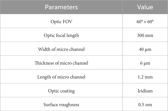
Table 1. Parameters of SXI.

2.3 The tangent fitting approach

In order to derive the 3-D magnetopause from a single X-ray image, Sun et al. (2020) proposed a novel method referred as the Tangent Fitting Approach (TFA), which is used to analyze the X-ray images in this paper. The TFA relies on two assumptions: (1) a parameterized functional form model which has the capacity to describe the magnetopause profiles, and (2) the locations of maximum intensity in the X-ray image correspond to the tangent directions of the magnetopause (Collier and Connor, 2018). The magnetopause model is a modified Shue et al. (1997) model, developed by Jorgensen et al. (2019), which takes into account the asymmetry of the magnetopause along the $y$ and $z$ axes of the GSM coordinate,

$r\left(\theta ,\varphi \right)=\frac{r_y\left(\theta \right)r_z\left(\theta \right)}{\sqrt{{\left[r_z\left(\theta \right)\cos \varphi \right]}^2+{\left[r_y\left(\theta \right)\sin \varphi \right]}^2}},(2)$

where $\theta$ is the angle between $\vec{r}$ and the $x$ axis, and $\varphi$ is the angle between the $y$ axis and the projection of $\vec{r}$ to the $y-z$ plane. In the equation, $r_y$ and $r_z$ are

$r_y\left(\theta \right)=r_0{\left(\frac{2}{1+\cos \theta }\right)}^{{\alpha }_y},(3)$

and

$r_z\left(\theta \right)=r_0{\left(\frac{2}{1+\cos \theta }\right)}^{{\alpha }_z},(4)$

Where $r_0$ is the standoff distance, and the level of tail flaring on the $x-y$ and $x-z$ plane is represented by ${\alpha }_y$ and ${\alpha }_z$, respectively. The three parameters $r_0$, ${\alpha }_y$, and ${\alpha }_z$ in Equations 3, 4 of this model describe the large-scale morphology of the magnetopause. For each combination of these parameters, the tangent directions of the magnetopause are calculated numerically. The basic idea of TFA is to compare the set of modeled tangent directions with the observed directions from X-ray images, in order to identify the optimal match. The tangent directions corresponding to this optimal match are used to determine the parameters that define the reconstructed magnetopause. By varying $r_0$, ${\alpha }_y$, and ${\alpha }_z$ within reasonable ranges, a set of magnetopause profiles can be generated. In this paper, realistic values are then calculated in Section 3 and presented in Table 3 as the “Truth” parameters. Based on that, these variables are varied within the following ranges: 4–10 $R_E$ for $r_0$ in 0.1 $R_E$ steps and 0–1 for ${\alpha }_y$ and ${\alpha }_z$ in 0.02 steps.

3 Results

Using the PPMLR-MHD code, we simulated the temporal variations of the magnetosphere from 15:00 UT on 10 May 2024 to 00:00 UT on 12 May 2024, with a time resolution of 1 min. By comparing these simulations with real-time solar wind data from the OMNI database (the OMNI data were obtained from the GSFC/SPDF OMNIWeb interface at https://omniweb.gsfc.nasa.gov), we selected five representative time points (shown in Figure 1; Table 2) to analyze the effects of solar wind parameters on the magnetopause position. In particular, we investigated the influence of solar wind number density $(N_{SW})$, as observed in Case 1 and Case 2 of Group 1; the orientation of the interplanetary magnetic field (IMF) component $B_Z$, as seen in Case 3 and Case 4 of Group 2; and the impact of extreme solar wind conditions, as represented in Case 5 of Group 3. The influence of solar wind number density can also be interpreted as the effect of solar wind proton flux, given that in the X-ray calculation Equation 1, the X-ray intensity is proportional to the product of solar wind number density and solar wind velocity (Zhang et al., 2023).

Figure 1

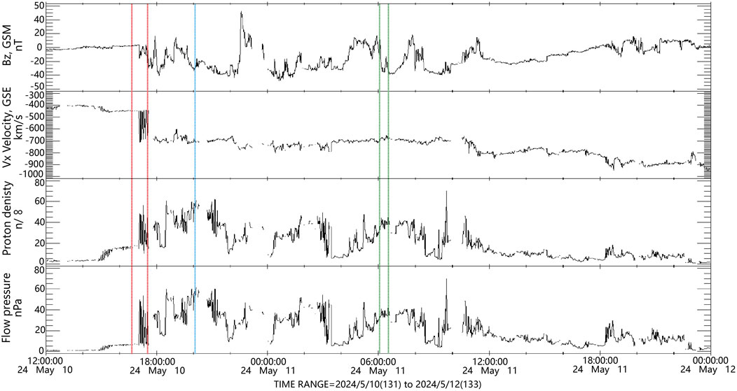
Figure 1. The solar wind conditions of IMF $B_Y$, $B_Z$, $V_X$ velocity, proton density, and flow pressure during the geomagnetic storm on 10–11 May 2024 from OMNI database (obtained from the GSFC/SPDF OMNIWeb interface at https://omniweb.gsfc.nasa.gov). The two red lines represent Group1 (Case1 and Case2) during the dynamic pressure pulse, where $N_{SW}$ increases; the two green lines represent Group2 (Case3 and Case4) during the southward turning of the IMF $B_Z$; and the blue line represents Group3 (Case5) under an extreme solar wind condition.

Table 2

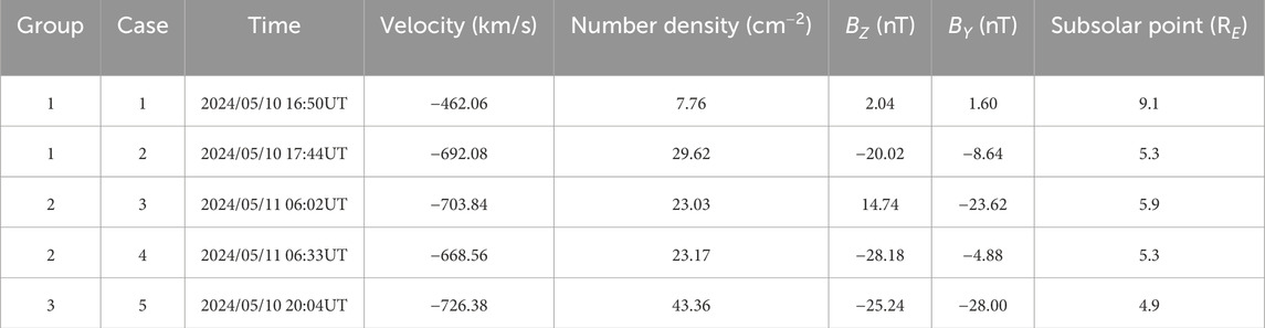
Table 2. Solar wind conditions for the studied simulation runs.

In this paper, we utilize the streamline method to locate the magnetopause position from the MHD simulation results, as shown by the white dashed line in Figure 2a4. More specifically, the streamline formula $\frac{dx}{Vx(x,y,z)}=\frac{dy}{Vy(x,y,z)}=\frac{dz}{Vz(x,y,z)}$ is applied in conjunction with the solar wind velocity components provided by the MHD code to identify the magnetopause position. This method generally returns a relatively smooth magnetopause profile, except in the vicinity of the subsolar point. To address these singularities, we conducted a detailed analysis of the variations in particle number density, thermal pressure, current density, and magnetic field to precisely pinpoint the magnetopause at the subsolar point. The locations of the subsolar point for Cases 1, 2, 3, 4, and 5 are 9.1, 5.3, 5.9, 5.3, and 4.9 $R_E$, respectively, as summarized in Table 2. It is worth noting that the compression of the subsolar point below the geostationary orbit is an unusual phenomenon and is not typically observed under standard solar wind conditions. Additionally, the cusp boundaries are delineated through the analysis of thermal pressure contours on a series of spherical shells extending from just above the inner boundary of the MHD code (r = 3.5 $R_E$) to the high-latitude magnetopause (Sun et al., 2019). On each spherical shell, the location with the maximum thermal pressure $P_{\mathit{max}}$ is defined as the center of the cusp region, while the cusp boundary is determined as the location where thermal pressure decreases to 60% of $P_{\mathit{max}}$.

Figure 2

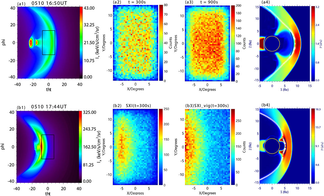
Figure 2. The X-ray images, SXI photon counts images, and reconstructed magnetopause images with a special viewing geometry. For Case 1 to 4 (A1–A4): (A1) the MHD simulated X-ray image; (A2, A3) the SXI photon counts images with exposure times of 300s and 900s, respectively; (A4) the contours of thermal pressure in the noon-meridian plane, with reconstructed magnetopause positions marked in the figures. The white dashed line represents the magnetopause position in MHD simulation, and the dark blue line indicates the reconstructed magnetopause derived from the photon counts images with exposure times of 900s. The yellow circle at the origin corresponds to a radial distance of 3 $R_E$. For Cases 2 to 4 (B1–B4): (B1) the MHD simulated X-ray image; (B2, B3) the SXI photon counts images, with (B3) incorporating the vignetting function; (B4) the contours of thermal pressure in the noon-meridian plane, with reconstructed magnetopause positions marked in the figures.

After determining the positions of both the magnetopause and the polar cusps, the X-ray emission within the magnetopause is set to zero. This modification allows for a more accurate calculation of the X-ray intensity throughout the magnetosphere. Assuming that there is an idealized telescope at a potential position of SMILE: (8.0, 0.0, 18.33) $R_E$ pointing towards (8.0, 0, 0) $R_E$, the X-ray images are then simulated for all the cases studied and discussed in the following section. This specific viewing geometry is chosen because the UVI and SXI instruments have a pointing angle of 23.5°, and the selected observation point is near the apogee of the SMILE candidate orbit, ensuring the telescope’s line of sight effectively covers the relevant regions of the magnetosphere and magnetosheath. All the SXI photon counts images account for the X-ray cosmic background, which is considered at 50 $KeV{s}^{-1}c{m}^{-2}s{r}^{-1}$. Unless otherwise specified, the exposure time is 300s.

3.1 The effect of the solar wind number density

Figure 2 shows the dynamic evolution of the X-ray intensity, photon counts and reconstructed magnetopause as the solar wind number density $(N_{SW})$ increases from 7.76 $c{m}^{-3}$ to 29.62 $c{m}^{-3}$. The images are in the $\theta \varphi$ coordinate system, with the axis labels $(\theta ,\varphi )$, where (0, 0) corresponds to the direction of the SXI pointing, and the positive $\theta$ axis points towards the Sun. The X and Z-axes are in the GSM coordinate system. The first row presents the results for Case 1, simulated on 2024/05/10 at 16:50 UT, while the second row shows the results for Case 2, simulated at 17:44 UT. Panels (a1, b1) show X-ray images, where the black rectangle marks the FOV of SXI on SMILE. Panels (a2, a3, b2, b3) are SXI photon counts images derived from X-ray intensity under different input parameters. The panels in the last column (a4, b4) show the contours of thermal pressure in the noon-meridian plane, with reconstructed magnetopause positions marked in the figures. The white dashed line represents the magnetopause position in MHD simulations, and the dark blue line indicates the reconstructed magnetopause derived from the photon counts images. The exposure times used to derive the magnetopause shown in (a4) and (b4) are 900s and 300s, respectively.

To better evaluate the reconstruction results, Equation 2 is used to directly fit the position and shape of the 3-D MHD magnetopause, which is labeled as “Truth.” Since the FOV of the X-ray image is $16°\times 27°$, which roughly corresponds to the region with $\theta \le 32°$ observed from this viewing geometry on the equatorial plane (where $\theta$ is defined by Equation 2), the portion of the magnetopause with $\theta \le 32°$ is used to fit and obtain the “Truth” parameters.

As $N_{SW}$ increases in Group1, a significant compression of the magnetopause is observed in the X-ray intensity images Figure 2a1, b1, with its position shifting from just inside the SMILE FOV to almost beyond it. A similar compression is also evident in the plasma thermal pressure from Figures 2a4–b4, where the subsolar point moves from 9.1 $R_E$ to 5.3 $R_E$.

For Case 1, where $N_{SW}\le 10c{m}^{-3}$, due to the relatively weak intensity of X-ray radiation under this solar wind condition, two exposure times, 300s and 900s, are considered for analysis. It is evident that, in this scenario, the intensity of the cosmic X-ray background surpasses that of the SWCX emissions, leading to the magnetospheric signal being obscured by the cosmic background noise. As a result, the distribution of maximum photon counts in the image does not represent the true position of the magnetopause, as shown in Figure 3A for “MHD” (blue circle) and “SXI” (green circle). Figure 3 the X-ray maximum intensity of MHD X-ray and SXI photon counts images. Panels (a), (b), (c), (d), and (e) correspond to Case 1, 2, 3, 4, and 5, respectively. The enlargement of the black box is the FOV of the SXI on SMILE. “MHD” refers to the X-ray maximum intensity of MHD X-ray images. “SXI” and “SXI-vig” represent X-ray maximum intensity of SXI photon counts images, with and without considering the vignetting effect. “SXI-vig-TFA” plots reconstruction magnetopause from photon counts image with vignetting function applied. Unless otherwise stated, the exposure time is 300s.

Figure 3

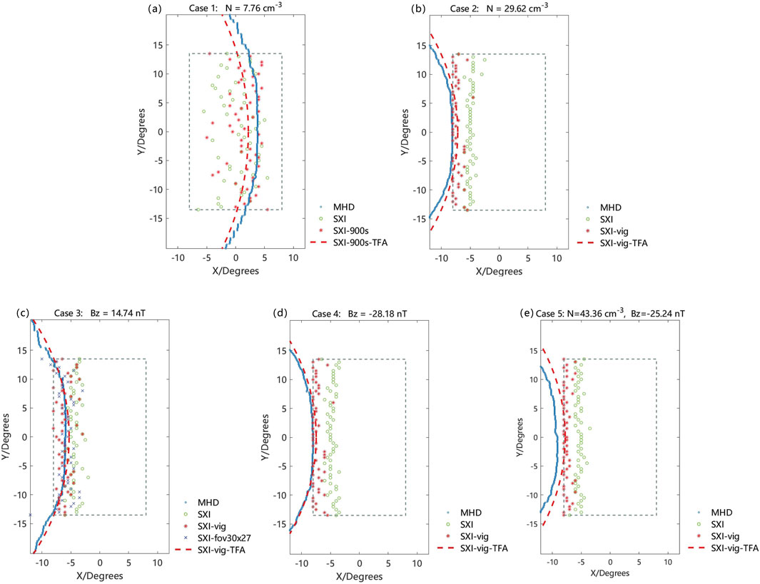
Figure 3. The X-ray maximum intensity of MHD X-ray and SXI photon counts images. Panels (A–E) correspond to Case 1, Case 2, Case 3, Case 4, and Case 5, respectively. The enlargement of the black box is the FOV of SXI on SMILE. “MHD” refers to the X-ray maximum intensity of MHD X-ray images. “SXI” and “SXI-vig” represent X-ray maximum intensity of SXI photon counts images, with and without considering the vignetting effect. “SXI-vig-TFA” plots reconstruction magnetopause from photon counts image with vignetting function applied. Unless otherwise stated, the exposure time is 300s. In panel (A), “SXI-900s-TFA” represents the reconstruction result from the “SXI-900s” image, which is derived from SXI photon counts with a 900s exposure time. In panel (C), “SXI-fov-$30°\times 27°$” refers to the SXI image derived from a 30$\times$ 27° FOV.

The magnetopause model parameters are then calculated using TFA reconstruction based on the SXI simulated photon counts images under two integration times. For the 300s exposure time, the photon counts image displayed in Figure 2a2 corresponds to the TFA parameters “SXI”: $r_0=8.4,{\alpha }_y=0.6,{\alpha }_z=1.0$. Similarly, for the 900s exposure time, as shown in Figure 2a3, the corresponding TFA parameters “SXI-900s” are: $r_0=8.7,{\alpha }_y=1.0,{\alpha }_z=0.1$. The numerical values of the TFA reconstruction parameters for all situations are listed in Table 3. When evaluated against the “Truth” values: $r_0=9.1,{\alpha }_y=0.64,{\alpha }_z=0.0$, the fitting parameters corresponding to the 900s exposure time demonstrate better consistency, with “SXI” (red asterisks) showing better agreement with “MHD” (blue circles) in Figure 3A compared to “SXI-900s” (green circles). The contours of thermal pressure in the noon-meridian plane with reconstructed magnetopause positions shown in Figure 2a4 is derived using the TFA parameters obtained from the 900s exposure time. It can be observed that the magnetopause derived from “SXI-900s” is closer to the Earth compared to the “Truth,” with an error of $△r_0=0.4,△{\alpha }_y=0.36,△{\alpha }_z=0.1$. The final rescontruction results is plotted by red dash line (“SXI-900s-TFA”) in Figure 3A and blue line in Figure 2a4. Hence, for lower solar wind number density, it can be concluded that a longer exposure time is required to determine the magnetopause location. Alternatively, image pre-processing (e.g., to reduce the influence of the cosmic background) can be considered for analysis of the X-ray image to enable a more accurate reconstruction of the magnetopause.

Table 3

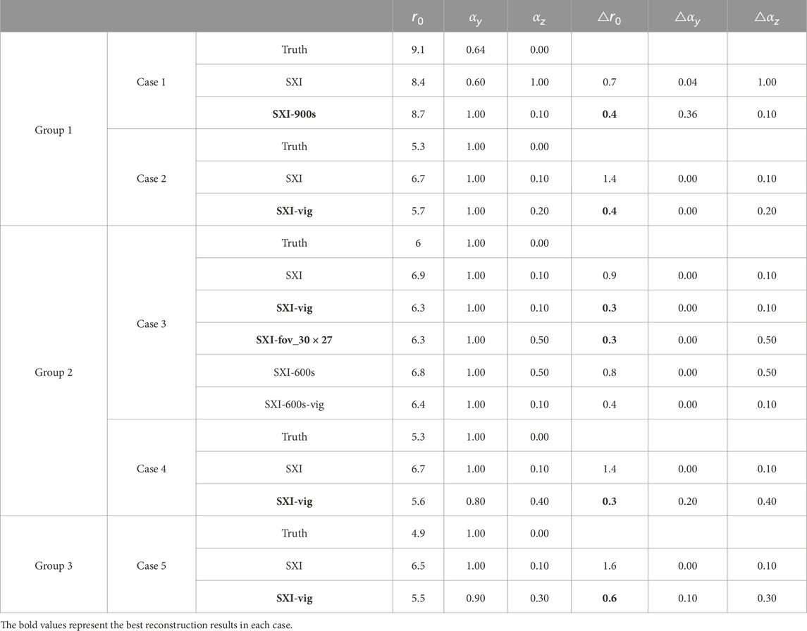
Table 3. Results of TFA reconstruction.

In Case 2, it can be seen in Figure 2b1 that when $N_{SW}$ is relatively large, the magnetopause is compressed almost outside the FOV of the payload. In other words, the photon signals from the magnetopause received by the SXI are located at the edge of the imaging FOV, as shown in Figure 2b2. “SXI” does not match the “MHD” in Figure 3B, which can be attributed to the vignetting effect, a phenomenon in which the SXI-detected X-ray intensity decreases towards the edges of the image compared to the center. This effect is caused by limitations in the optical system, such as the aperture size and the angular constraints of the lenses, which prevent incident photons at large field angles from fully reaching the sensor. In addition, the sensor’s response to photons varies with the angle of incidence, with reduced efficiency for photons rays entering at larger angles, particularly in the peripheral regions of the FOV. After considering the effect of vignetting function, the original X-ray signal and its maximum are plotted in Figure 2b3 and “SXI-vig” of Figure 3B, and the associated TFA parameters in Table 3 are labeled as “SXI-vig.” This function quantifies the variation of photons intensity as a function of position within the field of view and is commonly applied to model or correct for the vignetting effect induced by the optical system. Notably, this effect has been incorporated into the modeling of the spatially varying effective area of the SXI on SMILE (Sembay et al., 2024). After applying the vignetting correction, it can be seen that the position of the magnetopause in the photon counts image is more closely aligned with that in the X-ray image. It is also shown that the error between the “Truth” and reconstruction results is reduced from 1.4 $R_E$ to 0.4 $R_E$, and $△{\alpha }_y=0.0,△{\alpha }_z=0.2$. In cases of relatively large solar wind number density, it is not advisable to use the pixel points with photon counts maxima directly to determine the magnetopause position, as the presence of the vignetting function can significantly affect the accuracy of the maximum value determination. Therefore, it is necessary to first eliminate the vignetting effects before proceeding with the boundary tracing.

3.2 The effect of IMF $B_Z$ turning from north to south

Figure 4 illustrates the changes in Group2 when IMF $B_Z$ turns from northward to southward, from 14.74 nT to $-$28.18 nT, while the number density remains nearly constant. From 2024/05/11 at 06:02 UT to 06:33 UT, both the X-ray intensity and the contours of thermal pressure show significant increases, as illustrated in panels (a1, a4) to (b1, b4). This is accompanied by a pronounced compression of the magnetosheath, resulting in a sharper boundary. The “Truth” parameters are fitted with $r_0=6.0,{\alpha }_y=1.0,{\alpha }_z=0.0$ for the northern IMF $B_Z$ (Case3), while for the southern IMF $B_Z$ (Case4) $r_0=5.3,{\alpha }_y=1.0,{\alpha }_z=0.0$. Although, when $B_Z$ is southward for about 15 min, most regions are compressed beyond the FOV, except near the subsolar point. This can also be observed in the X-ray maximum intensity of the MHD X-ray and SXI photon counts images (Figures 3C, D). After considering the vignetting function, the subsolar point positions can still be determined based on the small portion of the magnetopause remaining within the FOV, which are consistent with the simulation results.

Figure 4

Figure 4. The X-ray images, SXI photon counts images, and reconstructed magnetopause images for Case 3 (A1–A4) and Case 4 (B1–B4). (A1, B1) the MHD simulated X-ray image; (A2, B2) the SXI photon counts images; (B2, B3) SXI photon counts images incorporating the vignetting function; (A4, B4) the contours of thermal pressure in the noon-meridian plane, with reconstructed magnetopause positions marked in the figures. The white dashed line represents the magnetopause position defined by streamline methods, and the dark blue line indicates the reconstructed magnetopause.

For Case 3, the error between the “Truth” and “SXI” is calculated as $△r_0=0.9,△{\alpha }_y=0.0,△{\alpha }_z=0.1$, while the error between the “Truth” and “SXI-vig” (which considered vignetting effect) is $△r_0=0.3,△{\alpha }_y=0.0,△{\alpha }_z=0.1$. The reduction in error $△r_0$ is evident, and photon counts maximum for “SXI-vig” matches the X-ray maximum intensity of MHD X-ray better than “SXI” in Figure 3C. This indicates the necessity of incorporating the vignetting function in future reconstruction studies, particularly under extreme solar wind conditions during geomagnetic storms. In this case, we also examine the results for another exposure time of 600s, both without and with vignetting function, referred to as “SXI-600s” and “SXI-600s-vig” in Table 3. When considering the vignetting effects, increasing the exposure time results in a slight change in error, and the improvement remains within the simulation grid spacing of 0.2 $R_E$. Therefore, for cases with higher solar wind proton flux, increasing the exposure time has a negligible impact on the results.

For Case 4, the error between “Truth” and “SXI” is $△r_0=1.4,△{\alpha }_y=0.0,△{\alpha }_z=0.1$, as for “SXI-vig” it is $△r_0=0.3,△{\alpha }_y=0.2,△{\alpha }_z=0.4$. Although the errors in ${\alpha }_y$ and ${\alpha }_z$ exhibit some increase, it should be noted that the FOV of the SXI primarily focuses on the dayside of the magnetosphere and does not extend sufficiently to capture the flanks and tail regions, the reconstructed parameters and exhibit less sensitivity compared to $r_0$ (Sun et al., 2020). Nevertheless, $r_0$ remains the most critical parameter for analysis, and the results considering vignetting effects show a better agreement with the simulated results.

3.3 The effect of extreme solar wind conditions

Figure 5 presents Case 5, an extreme solar wind condition where solar wind number density $(N_{SW})$ reaches a high value of 43.36 $c{m}^{-3}$, while the IMF $B_Z$ is southward with a magnitude of 25 nT. In this case, the magnetopause erosion is significant. In Figure 5A1, A4, it can be seen that the cusps are compressed into very small regions, making them not very distinct. The footprints of the cusps are at a low latitude, and cusps altitude are also very low. The positions of the magnetopause and cusp regions are located outside the FOV, a pattern that is more distinctly observable in the maximum X-ray intensity, as depicted in Figure 3E. Due to the low position of the bow shock at this moment, a time delay of 4 min has been considered. The “Truth” parameters are fitted with $r_0=4.9,{\alpha }_y=1.0,{\alpha }_z=0.0$ that show a particularly strong magnetopause erosion. The “SXI” parameters, as plotted in Figure 5A2, are $r_0=6.5,{\alpha }_y=1.0,{\alpha }_z=0.1$, while “SXI-vig” parameters, as plotted in Figure 5A3, are $r_0=5.5,{\alpha }_y=0.9,{\alpha }_z=0.3$, with errors in $△r_0$ are 1.6 $R_E$ and 0.6 $R_E$, respectively. Given that the pixel size of the SXI is about 0.5°, corresponding to a spatial accuracy of about 0.2 $R_E$ in spatial scales, the variation of $△r_0$ across different scenarios exceeds the instrument’s error, regardless of whether the vignetting function is considered. At this point, the introduction of the vignetting function is no longer applicable, and it may be necessary to adjust the instrument’s line of sight to achieve a three-dimensional large-scale reconstruction of the magnetopause.

Figure 5

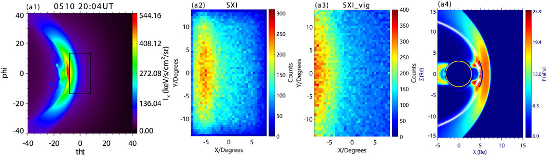
Figure 5. The X-ray images, SXI photon counts images, and reconstructed magnetopause images for Case 5. (A1) the MHD simulated X-ray image; (A2) the SXI photon counts images; (A3) the SXI photon counts images incorporating the vignetting function; (A4) the contours of thermal pressure in the noon-meridian plane, with reconstructed magnetopause positions marked in the figures.

4 Discussion

Based on the results of the TFA reconstruction parameters, the reconstructed magnetopause positions in the Cases (2, 3, 4) are located closer to the subsolar region compared to the true values. This is related to the fact that, in these cases, the magnetopause is located at the edge of the instrument’s FOV, which affects the reconstruction. It is therefore essential to take the vignetting effect into account in such scenarios. Upon incorporating the vignetting function, the reconstructing error in $r_0$ reduce from more than 1 $R_E$ to less than 0.5 $R_E$. In Cases 2 and 4, where only a small portion of the magnetopause is within the FOV, it is reasonable that reconstruction results for ${\alpha }_y$ and ${\alpha }_z$ are not as good as $r_0$. Furthermore, we examine a hypothetical scenario in which the FOV is extended from $16°\times 27°$ to $30°\times 27°$ and calculate corresponding 3-D magnetopause parameters for Case 3. The comparison between the results obtained with and without the vignetting function reveals that the errors in $△r_0$ is 0.0 $R_E$. Thus, for cases such as 2, 3, and 4, where the magnetopause is located near the edge of the FOV, the introduction of the vignetting function effectively declines the impact of edge effects, significantly improving the precision of the final reconstructed magnetopause near the subsolar point.

With regard to the instrument exposure time, the analysis of Case 1 and Case 3 shows that under conditions of relatively low solar wind number density, where X-ray emissions are weak, an increase in exposure time contributes to a reduction in reconstruction errors. Therefore, for scenarios with lower solar wind number densities, future TFA applications should consider image preprocessing techniques, such as increasing exposure time or reducing the influence of cosmic background, to improve the accuracy of magnetopause reconstruction.

5 Conclusion

In this paper, we conduct simulations of dynamic soft X-ray images generated by SWCX in the Earth’s magnetosheath and cusps using the PPMLR-MHD model, as well as photon counts images derived from SXI simulations, during the super storm of 10-11 May 2024. The analysis focuses on evaluating the effectiveness of the SXI simulation and the Tangent Fitting Approach (TFA) in reconstructing the 3-D structure of magnetopause under dynamic and non-standard solar wind conditions, with a particular emphasis on the magnetopause near the subsolar point.

The results demonstrate that when the magnetopause is within the FOV, these methods can reconstruct a precise subsolar magnetopause with errors within 0.5 $R_E$, which satisfies the scientific requirements for the SMILE mission. Specifically, three groups of solar wind conditions are analyzed: varying solar wind number density or solar wind proton flux (Group 1), different IMF $B_Z$ orientations (Group 2), and an extreme condition with high number density and strong southward IMF $B_Z$ (Group 3). Nevertheless, due to the limited FOV of the SXI, in certain scenarios the magnetopause is located at the edge of the FOV, restricting the observable region to only a small part near the subsolar point. As a result, the level of magnetopause tail flaring in the x-y and x-z planes is less detailed than subsolar region. After accounting for the vignetting effect in SXI imaging, the TFA-derived subsolar magnetopause from the SXI simulation exhibits good agreement with the true profile. During the dynamic pressure pulse, $N_{SW}$ increases, resulting in an erosion of the magnetopause by 3.8 $R_E$. Simultaneously, when the IMF $B_Z$ turns southward for about 15 min, the corresponding compression is 0.7 $R_E$. During extreme solar wind condition, the magnetopause location is compressed to 4.9 $R_E$, which exceeds the FOV of SXI. At this point, it may be necessary to adjust the instrument’s line of sight.

In conclusion, this study shows that: (1) the dynamic variations of the magnetopause during the geomagnetic storm are effectively captured by X-ray imaging; (2) the reconstruction results for the magnetopause location are provided in a quantitative description, offering valuable insights into its position and behavior during the storm; and (3) under the solar wind conditions associated with this particular geomagnetic storm, the observational limits of the SMILE SXI have essentially been reached. These configurations of the magnetopause in Case 2 and Case 4 reflect its maximum compression states under the current viewing pointing of SMILE.

Data availability statement

The raw data supporting the conclusions of this article will be made available by the authors, without undue reservation.

Author contributions

YuG: Writing–original draft. TS: Writing–review and editing. BT: Writing–review and editing. YiG: Writing–review and editing. SS: Writing–review and editing. CW: Writing–review and editing.

Funding

The author(s) declare that financial support was received for the research, authorship, and/or publication of this article. This work was supported by the National Natural Science Foundation of China (Grant Nos 42322408, 42188101, 42122032, and 42074202), and the Climbing Program of NSSC (E4PD3005).

Conflict of interest

The authors declare that the research was conducted in the absence of any commercial or financial relationships that could be construed as a potential conflict of interest.

Generative AI statement

The author(s) declare that no Generative AI was used in the creation of this manuscript.

Publisher’s note

All claims expressed in this article are solely those of the authors and do not necessarily represent those of their affiliated organizations, or those of the publisher, the editors and the reviewers. Any product that may be evaluated in this article, or claim that may be made by its manufacturer, is not guaranteed or endorsed by the publisher.

References

Branduardi-Raymont, G., Elsner, R. F., Gladstone, R., Ramsay, G., Rodriguez, P., Soria, R., et al. (2004). First observation of jupiter by XMM-Newton. Astronomy and Astrophysics 424, 331–337. doi:10.1051/0004-6361:20041149

CrossRef Full Text | Google Scholar

Branduardi-Raymont, G., Wang, C., Escoubet, C., Adamovic, M., Berthomier, M., Carter, J. A., et al. (2018). SMILE definition study report (red book). ESA/SCI: European Space Agency. doi:10.5270/esa.smile.definition_study_report-2018-12

CrossRef Full Text | Google Scholar

Carter, J. A., and Sembay, S. (2008). Identifying XMM-Newton observations affected by solar wind charge exchange. Part I. Astronomy and Astrophysics 489, 837–848. doi:10.1051/0004-6361:200809997

CrossRef Full Text | Google Scholar

Carter, J. A., Sembay, S., and Read, A. M. (2010). A high charge state coronal mass ejection seen through solar wind charge exchange emission as detected by XMM-Newton. Mon. Notices R. Astronomical Soc. 402, 867–878. doi:10.1111/j.1365-2966.2009.15985.x

CrossRef Full Text | Google Scholar

Collier, M. R., and Connor, H. K. (2018). Magnetopause surface reconstruction from tangent vector observations. J. Geophys. Res. Space Phys. 123 (10), 189–210. doi:10.1029/2018JA025763

CrossRef Full Text | Google Scholar

Collier, M. R., Snowden, S. L., Sarantos, M., Benna, M., Carter, J. A., Cravens, T. E., et al. (2014). On lunar exospheric column densities and solar wind access beyond the terminator from ROSAT soft X-ray observations of solar wind charge exchange. J. Geophys. Res. Planets 119, 1459–1478. doi:10.1002/2014JE004628

CrossRef Full Text | Google Scholar

Connor, H. K., Sibeck, D. G., Collier, M. R., Baliukin, I. I., Branduardi-Raymont, G., Brandt, P. C., et al. (2021). Soft X-ray and ENA imaging of the Earth’s dayside magnetosphere. J. Geophys. Res. Space Phys. 126, e2020JA028816. doi:10.1029/2020JA028816

PubMed Abstract | CrossRef Full Text | Google Scholar

Cravens, T. E. (1997). Comet Hyakutake x-ray source: charge transfer of solar wind heavy ions. Geophys. Res. Lett. 24, 105–108. doi:10.1029/96GL03780

CrossRef Full Text | Google Scholar

Cravens, T. E. (2000). Heliospheric X-ray emission associated with charge transfer of the solar wind with interstellar neutrals. Astrophysical Journa 532, L153–L156. doi:10.1086/312574

PubMed Abstract | CrossRef Full Text | Google Scholar

Cravens, T. E., Robertson, I. P., and Snowden, S. L. (2001). Temporal variations of geocoronal and heliospheric X-ray emission associated with the solar wind interaction with neutrals. J. Geophys. Res. Space Phys. 106, 24883–24892. doi:10.1029/2000JA000461

CrossRef Full Text | Google Scholar

Dennerl, K., Lisse, C., Bhardwaj, A., Burwitz, V., Englhauser, J., Gunell, H., et al. (2006). First observation of Mars with XMM-Newton. 451, 709, 722. doi:10.1051/0004-6361:20054253

CrossRef Full Text | Google Scholar

Guo, Y., Sun, T., and Sembay, S. (2022). Deriving the magnetopause position from wide field-of-view soft X-ray imager simulation. Sci. China Earth Sci. 65, 1–11. doi:10.1007/s11430-021-9937-y

CrossRef Full Text | Google Scholar

Hodges, J., and Richard, R. (1994). Monte Carlo simulation of the terrestrial hydrogen exosphere. J. Geophys. Res. Space Phys. 99, 23229–23247. doi:10.1029/94JA02183

CrossRef Full Text | Google Scholar

Hu, Y. Q., Guo, X. C., and Wang, C. (2007). On the ionospheric and reconnection potentials of the earth: results from global MHD simulations. J. Geophys. Res. Space Phys. 112. doi:10.1029/2006JA012145

CrossRef Full Text | Google Scholar

Jorgensen, A. M., Sun, T., Wang, C., Dai, L., Sembay, S., Wei, F., et al. (2019). Boundary detection in three dimensions with application to the SMILE mission: the effect of photon noise. J. Geophys. Res. Space Phys. 124, 4365–4383. doi:10.1029/2018JA025919

CrossRef Full Text | Google Scholar

Lisse, C. M., Dennerl, K., Englhauser, J., Harden, M., Marshall, F. E., Mumma, M. J., et al. (1996). Discovery of X-ray and extreme ultraviolet emission from Comet C/Hyakutake 1996 B2. Science 274, 205–209. doi:10.1126/science.274.5285.205

CrossRef Full Text | Google Scholar

Peng, S., Ye, Y., Wei, F., Yang, Z., Guo, Y., and Sun, T. (2018). Numerical model built for the simulation of the earth magnetopause by lobster-eye-type soft X-ray imager onboard SMILE satellite. Opt. Express 26, 15138. doi:10.1364/OE.26.015138

PubMed Abstract | CrossRef Full Text | Google Scholar

Samsonov, A., Branduardi-Raymont, G., Sembay, S., Read, A., Sibeck, D., and Rastaetter, L. (2024). Simulation of the SMILE Soft X-ray Imager response to a southward interplanetary magnetic field turning. Earth Planet. Phys. 8, 39–46. doi:10.26464/epp2023058

CrossRef Full Text | Google Scholar

Samsonov, A., Carter, J. A., Read, A., Sembay, S., Branduardi-Raymont, G., Sibeck, D., et al. (2022a). Finding magnetopause standoff distance using a soft X-Ray Imager: 1. magnetospheric masking. J. Geophys. Res. Space Phys. 127, e2022JA030848. doi:10.1029/2022JA030848

CrossRef Full Text | Google Scholar

Samsonov, A., Sembay, S., Read, A., Carter, J. A., Branduardi-Raymont, G., Sibeck, D., et al. (2022b). Finding magnetopause standoff distance using a Soft X-ray Imager: 2. methods to analyze 2-D X-ray images. J. Geophys. Res. Space Phys. 127, e2022JA030850. doi:10.1029/2022JA030850

CrossRef Full Text | Google Scholar

Sembay, S., Alme, A. L., Agnolon, D., Arnold, T., Beardmore, A., Margeli, A. B. B., et al. (2024). The soft X-ray imager (SXI) on the SMILE mission. Earth Planet. Phys. 8, 5–14. doi:10.26464/epp2023067

CrossRef Full Text | Google Scholar

Shue, J.-H., Chao, J. K., Fu, H. C., Russell, C. T., Song, P., Khurana, K. K., et al. (1997). A new functional form to study the solar wind control of the magnetopause size and shape. J. Geophys. Res. Space Phys. 102, 9497–9511. doi:10.1029/97JA00196

CrossRef Full Text | Google Scholar

Sun, T., Wang, C., Connor, H. K., Jorgensen, A. M., and Sembay, S. (2020). Deriving the magnetopause position from the soft X-ray image by using the tangent fitting approach. J. Geophys. Res. Space Phys. 125, e2020JA028169. doi:10.1029/2020JA028169

CrossRef Full Text | Google Scholar

Sun, T., Wang, C., Sembay, S., Lopez, R., Escoubet, C., Branduardi-Raymont, G., et al. (2019). Soft X-ray imaging of the magnetosheath and cusps under different solar wind conditions: MHD simulations. J. Geophys. Res. Space Phys. 124, 2435–2450. doi:10.1029/2018JA026093

CrossRef Full Text | Google Scholar

Sun, T., Wang, X., and Wang, C. (2021). Tangent directions of the cusp boundary derived from the simulated soft X-ray image. J. Geophys. Res. Space Phys. 126, e2020JA028314. doi:10.1029/2020JA028314

CrossRef Full Text | Google Scholar

Sun, T. R., Wang, C., Wei, F., and Sembay, S. (2015). X-ray imaging of Kelvin-Helmholtz waves at the magnetopause. J. Geophys. Res. Space Phys. 120, 266–275. doi:10.1002/2014JA020497

CrossRef Full Text | Google Scholar

Tulasi Ram, S., Veenadhari, B., Dimri, A. P., Bulusu, J., Bagiya, M., Gurubaran, S., et al. (2024). Super-intense geomagnetic storm on 10–11 May 2024: possible mechanisms and impacts. Space weather. 22, e2024SW004126. doi:10.1029/2024sw004126

PubMed Abstract | CrossRef Full Text | Google Scholar

Wang, C., and Branduardi-Raymont, G. (2018). Progress of solar wind magnetosphere ionosphere Link explorer (SMILE) mission. Chin. J. Space Sci. 38, 657. doi:10.11728/cjss2018.05.657

CrossRef Full Text | Google Scholar

Wang, R. C., Jorgensen, A. M., Li, D., Sun, T., Yang, Z., and Peng, X. (2024). An adaptive X-Ray dynamic image estimation method based on OMNI solar wind parameters and SXI simulated observations. Space weather. 22, e2024SW004040. doi:10.1029/2024SW004040

CrossRef Full Text | Google Scholar

Wargelin, B. J., Markevitch, M., Juda, M., Kharchenko, V., Edgar, R., and Dalgarno, A. (2004). Chandra observations of the “Dark” moon and geocoronal solar wind charge transfer. Astrophysical J. 607, 596–610. doi:10.1086/383410

CrossRef Full Text | Google Scholar

Whittaker, I. C., and Sembay, S. (2016). A comparison of empirical and experimental O⁷⁺, O⁸⁺, and O/H values, with applications to terrestrial solar wind charge exchange. Geophys. Res. Lett. 43, 7328–7337. doi:10.1002/2016GL069914

CrossRef Full Text | Google Scholar

Xu, Q., Tang, B., Sun, T., Li, W., Zhang, X., Wei, F., et al. (2022). Modeling of the subsolar magnetopause motion under interplanetary magnetic field southward turning. Space weather. 20, e2022SW003250. doi:10.1029/2022SW003250

CrossRef Full Text | Google Scholar

Zhang, Y., Sun, T., Carter, J. A., Sembay, S., Koutroumpa, D., Ji, L., et al. (2023). Dynamical response of solar wind charge exchange soft X-ray emission in Earth’s magnetosphere to the solar wind proton flux. Earth’s Magnetos. Sol. Wind Prot. Flux 948, 69. doi:10.3847/1538-4357/acc326

CrossRef Full Text | Google Scholar