The first analysis of the outward H fluxes measured by IBEX-Lo in 20–50 RE geocentric distances

In this study, we analyze the energetic neutral atom (ENA) observations measured in the lowest energy channel (10–21 eV) of the IBEX-Lo instrument on Interstellar Boundary Explorer (IBEX) during two spring seasons, day of year (DOY) 101–146, 2009, and DOY 88–178, 2013, confirming the existence of outward hydrogen (H) fluxes at 15 eV. The outward H flux decreases slightly with distance, showing an intensity of approximately 10⁶ cm⁻² s⁻¹ sr⁻¹ keV⁻¹. Results also suggest that the outward H fluxes are not influenced by solar radio flux. We compute the expected H ENA fluxes at 15 eV using ion flux measurements from the Helium, Oxygen, Proton, and Electron (HOPE) mass spectrometer aboard the Radiation Belt Storm Probes (RBSP) during the corresponding period of the 2013 spring season, combined with a simple exospheric density model ($n_{\mathrm{H}}=n_{\mathrm{H}0}{\left(r_0/r\right)}^3$, where $r_0=10$ R_E). The expected ENA fluxes similarly show a decrease in the intensity with increasing geocentric distance, which is on the order of 10⁵–10⁶ cm^-2 s⁻¹ sr⁻¹ keV⁻¹. These consistent features suggest that the outward H fluxes observed by IBEX-Lo are closely related to escaping H ENAs produced within the inner exosphere (<4 R_E).

1 Introduction

NASA’s Interstellar Boundary Explorer (IBEX) mission aims to discover the global interaction between solar winds and the local interstellar medium (McComas et al., 2009). IBEX can also provide energy-resolved terrestrial hydrogen (H) energetic neutral atom (ENA) observations due to the following observation configurations. First, the IBEX spacecraft follows a highly elliptical and nearly equatorial orbit around Earth. Due to this elongated orbit, IBEX routinely views Earth’s magnetosphere from side-viewing vantage points from March to June (spring) and September to December (fall) (see Figure 1 in Hart et al., 2021). Second, the spacecraft spins with a Sun-pointing rotation axis, and its ENA instruments have a ∼7° full-width-half-max (FWHM) ENA acceptance angle (McComas et al., 2009). This configuration results in its field-of-view (FOV) covering a swath of the sky perpendicular to the Sun-pointed spin-axis. Finally, IBEX is equipped with two single-pixel ENA instruments that measure neutral atoms in the energy ranges of ∼0.01–2 keV in eight energy steps of IBEX-Lo (Fuselier et al., 2009) and ∼0.3–6 keV in six energy steps of IBEX-Hi (Funsten et al., 2009). The energy ranges of IBEX correspond to the energies of the major plasma populations in the magnetosphere (Chappell et al., 2008), enabling it to provide energy-resolved observations of terrestrial ENAs, which are produced by charge exchange between plasma ions and ambient neutral atoms.

Figure 1

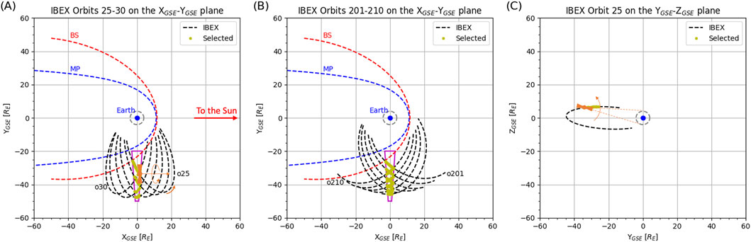
Figure 1. Trajectories of IBEX: (A) IBEX Orbits 25–30 (Case 2009: 4/11/2009–5/26/2009) projected on the X_GSE–Y_GSE plane; (B) IBEX Orbits 201–210 (Case 2013: 3/29/2013–6/27/2013) projected on the X_GSE–Y_GSE plane; (C) IBEX Orbit 25 projected on the Y_GSE–Z_GSE plane. The selected trajectory segments are marked as yellow dots, and the selection zones are indicated as magenta trapezoids. The model magnetopause (Shue et al., 1998) and bow shock (Jerab et al., 2004) are represented as blue and red dashed lines, respectively.

For the past decade, IBEX has provided not only heliospheric ENA observations but also imaging data of distant magnetospheric regions and energy-resolved observations of terrestrial ENAs. IBEX-Hi terrestrial ENA observations have been analyzed to study terrestrial ENA sources, including the Earth’s subsolar magnetopause (Fuselier et al., 2010; Fuselier et al., 2020), the terrestrial plasma sheet (Dayeh et al., 2015; Fuselier et al., 2015; McComas et al., 2011), magnetospheric cusps (Petrinec et al., 2011), and the dayside magnetosheath (Ogasawara et al., 2013). Previous literature shows that IBEX terrestrial ENA observations can provide a unique global viewing perspective of the magnetosphere, complementing in situ measurements and, thus, enhancing the understanding of magnetospheric plasma regions and processes on both micro and macro scales.

Plasma populations with energy ranging from 0.1 eV to hundreds of eV are found in the magnetosphere (Chappell et al., 2008). These ions can exchange electrons with ambient exospheric H atoms (∼0.01 eV), becoming charge-exchange-induced H ENAs that can escape the Earth’s gravitational influence and be measured by the IBEX-Lo ENA instrument. Studying the escaping neutral atoms is key to understanding the role of non-thermal atoms in Earth’s atmospheric loss (Shizgal and Arkos, 1996). The IBEX-Lo terrestrial ENA observation provides a unique tool for investigating low-energy terrestrial ENAs that escape the Earth’s atmosphere. However, the IBEX-Lo terrestrial ENA observations have not yet been explored. This study examines whether the IBEX-Lo terrestrial H ENA observations provide the in situ measurements of charge-exchange-induced H ENAs generated in the inner exosphere (<4 R_E).

This paper is organized as follows. Section 2 describes the IBEX-Lo ENA dataset and the data selection and analysis methodology. Section 3 discusses the IBEX 15 eV ENA observations and compares the observed fluxes with simulated fluxes obtained from a simple ENA flux model. Finally, Section 4 presents our summary.

2 Materials and methods

2.1 IBEX-Lo ENA data

The IBEX observation configurations provide a perfect platform for observing ENA emissions from the Earth’s magnetosphere over long periods and from distances up to ∼50 R_E. IBEX views the magnetosphere from the side, observing continuous ∼7 ° × 360 ° vertical swaths of the sky at a resolution of ∼14 s per full swath, covering an overlapping energy range of ∼0.01–∼2 keV (IBEX-Lo) and ∼0.3–∼6 keV (IBEX-Hi) (McComas et al., 2009). These swaths combine spatial and temporal information and are used to construct composite ENA images of the Earth’s magnetosphere under different solar wind and interplanetary magnetic field conditions.

This study uses the IBEX-Lo ENA histogram datasets, which are publicly available through the IBEX Raw Data Release (https://ibex.princeton.edu). The numbered IBEX Data Releases focus on heliospheric ENAs, and the ENAs from the intervals when the FOV crossed the magnetosphere are considered contaminated and are removed. Thus, in this study, we use the Raw Data Release, which includes all IBEX observations, even those from the intervals when the FOV crossed the magnetosphere. Those data are carefully processed to select the restricted time intervals that meet the study requirements, as described in Section 2.2. The ENA histogram dataset consists of count histograms for each orbit and eight energy steps (E-steps) with a width of ΔE/E ∼ 0.7. Each count histogram (i.e., vertical swath) comprises 60 6° angular bins accumulated over 64 spins, resulting in a cadence of ∼15 min. This study combines four swaths to achieve a 1-h cadence (256 spins × ∼14 s/spin = ∼60 min/swath) to improve the statistical reliability. Each count histogram includes the number of events per angular bin, event type, cadence start time, spacecraft ephemeris, and spacecraft pointing information.

2.2 IBEX data selection

We use the ENA histogram data measured at E-step 1 (E_cen = 15 eV, E_−FWHM = 11 eV, and E_+FWHM = 21 eV; Fuselier et al., 2009) during two time periods: Day of Year (DOY) 101–146, 2009 (Case 2009; Orbits 25–30) and DOY 88–178, 2013 (Case 2013; Orbits 201–210) to study the connection of the IBEX-Lo measurements at the lowest E-step to the low-energy H ENAs produced in the inner exosphere as well as its variation in different solar radio fluxes. We consider the inner exosphere to be a sphere of 4 R_E geocentric radius.

2.2.1 Selected IBEX trajectories and an example histogram plot

This study focused on the 2009 spring season because the IBEX-Lo instrument viewed the inner exosphere from the dawn region during this period, providing the first ENA histogram datasets that are possibly associated with the neutral H atoms escaping from the inner exosphere. This period also corresponds to the solar minimum conditions, with an F10.7 index of approximately 70. Unfortunately, there are no in situ ion flux observations at the low energies corresponding to E-step 1 of the IBEX-Lo instrument near the inner exosphere during the 2009 spring season. Therefore, we cannot directly compare the IBEX-Lo ENA observations taken in the 2009 spring season with simulated ENA fluxes computed from in situ ion flux measurements. To address this limitation, the 2013 spring season was selected for analysis of IBEX-Lo measurements at E-step 1, specifically when the IBEX-Lo FOV crossed the inner exosphere. The Helium, Oxygen, Proton, and Electron (HOPE) mass spectrometer aboard the Radiation Belt Storm Probes (RBSP) provided the in situ measurements of ion fluxes at 15 eV during the period corresponding to the 2013 spring season. The 2013 spring season represents solar maximum conditions, with an F10.7 index ranging from approximately 100 to 150.

Figure 1 illustrates the trajectories of IBEX during the 2009 and 2013 spring seasons. Panels (A) and (B) display IBEX Orbits 25–30 and 201–210, respectively, which are projected onto the X_GSE–Y_GSE plane in the Geocentric Solar Ecliptic (GSE) coordinate system. Panel (C) shows IBEX Orbit 25 projected onto the Y_GSE–Z_GSE plane. The black dashed lines represent the spacecraft trajectories. At the same time, the yellow dots highlight the selected trajectory segment within the selection zone (indicated by the magenta trapezoid), where the IBEX FOV crosses the inner exosphere. The orange diagram represents the IBEX spacecraft, with its spin axis depicted as a straight orange arrow. Two additional orange arrows indicate the directions of the spacecraft’s rotation and forward motion along its trajectory (counterclockwise). The gray dashed circle represents the inner exosphere, which is defined as a geocentric sphere with a radius of 4 R_E. The blue curve marks the boundary of the model magnetopause, which is calculated using Shue’s magnetopause model (see Equation 8 in Shue et al., 1998) with an interplanetary magnetic field (IMF) component B_{IMF, Z} = 0 nT and solar wind dynamic pressure P_sw = 1.1 nPa. The red dashed curve represents the boundary of the model bow shock, which is determined using Jerab’s bow shock model (see Equation 10 in Jerab et al., 2004) with an IMF strength B_IMF = 6 nT, solar wind flow speed V_sw = 400 km/s, solar wind proton number density N_sw = 6 cm⁻³, and Alfven Mach number M_a = 10. Here, typical solar wind parameters are used because we use the boundaries of the model magnetopause, and bow shocks serve as guidelines for the selection criteria.

For each orbit, the IBEX ENA histogram dataset provides count histograms as a function of time and angle, which are used to generate histogram plots. Figure 2 showcases an example histogram dataset measured by IBEX-Lo during Orbit 25 (DOY 101-108, 2009) at E-step 1. Panel (A) displays a histogram plot of measured neutral atoms, with the horizontal axis representing the observation time and the vertical axis showing the angle relative to the north ecliptic pole (NEP): $C_{i,j}\left(t_i,{\theta }_j\right)$, where $t_i$ is a time tick of swath i and ${\theta }_j$ is a center angle of angular bin j. Each vertical swath corresponds to a 1-h observation cadence. The vertical red dashed lines denote the restricted time interval, while the horizontal red dashed lines indicate the restricted angle range, as described in Section 2.2.3. Panel (B) shows the accumulated counts per swath over the angle range of 210°–308° as a function of time (black curve): $C_i^{\text{angle}}\left(t_i\right)={\displaystyle {\sum }_j}{C}_{i,j}\left(t_i,{\theta }_j\right)$. This angle range was chosen to capture emissions from the Earth’s side. The blue curve represents solar wind dynamic pressures during Orbit 25, obtained from the OMNIWeb database. The green dashed line indicates the background level described in Section 2.2.3. Panel (C) presents the accumulated counts per 6 ° × 6 ° bin over different periods as a function of the NEP angle: $C_j^{\text{time}}\left({\theta }_j\right)={\displaystyle {\sum }_i}{C}_{i,j}\left(t_i,{\theta }_j\right)/N_{\text{swath}}$, where N_swath is the number of swaths in the selected period. The red solid line represents the accumulated counts over the entire orbit period (approximately 7 days). The black line corresponds to the counts in the first half-day (DOY 101.5–102) when the spacecraft was in the magnetosheath, the blue line shows the counts from DOY 102–108 when the spacecraft was outside the magnetosheath, and the green line represents the counts from the restricted time interval. The dotted curves show the Gaussian function to fit the accumulated counts within the 210°–308° angle range for each case. The optimal values for the parameters are written in the caption of Figure 2. The Gaussian distribution function could be a reasonable first assumption to characterize the accumulated counts over different periods. For instance, the accumulated counts in the magnetosheath have a broad width because the emissions could result from in situ measurements of the energetic ions in the magnetosheath (Hart et al., 2021). In contrast, the accumulated counts outside the magnetosheath have a narrower distribution along the NEP angle of 270°. This narrow distribution could be an indicator of emissions resulting from ENAs originating from the Earth’s magnetosphere (Dayeh et al., 2015) and magnetosheath (Ogasawara et al., 2013). We discuss these emissions in detail in Section 2.2.2. Finally, Panel (D) illustrates the trajectory of IBEX during Orbit 25, formatted similarly to Figure 1.

Figure 2

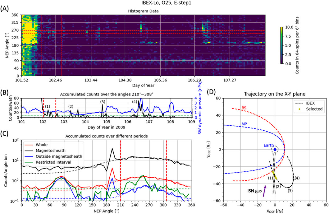
Figure 2. Showcase of an example histogram dataset for Orbit 25 at E-step 1. (A) IBEX-Lo ENA histogram plot as a function of the NEP angle (sixty 6° bins) and spin accumulated in 256-spin (∼1 h) × 6° bins. The red vertical dashed lines represent the restricted time interval, and the red horizontal lines indicate the restricted angle range. (B) Accumulated counts per swath over the angle range of 210°–308° as a function of time (black curve) and the solar wind dynamic pressure during the same period of Orbit 25 (blue curve). The green dashed line indicates the background level. (C) Accumulated counts per angle bin over different periods as a function of the NEP angle (red for the entire orbit period, black for DOY 101.5–102, blue for DOY 102–108, and green for the restricted time interval). The dotted curves show the Gaussian fits to the accumulated counts within the 210°–308° angle range. The optimal values of a center angle and a standard deviation are (259°, 49°) for the entire orbit period, (254°, 62°) for the magnetosheath signal, (266°, 29°) for outside the magnetosheath, and (255°, 7°) for the restricted time interval. (D) Trajectory of IBEX during Orbit 25, formatted similarly to Figure 1.

2.2.2 Possible background sources

IBEX-Lo ENA observations are line-of-sight (LOS) integrated measurements, meaning the resulting ENA histograms may include emissions from various sources such as interstellar neutral (ISN) gas (Moebius et al., 2009), heliospheric neutral atoms (including the globally distributed flux and the IBEX ribbon; McComas et al., 2012), and terrestrial ENAs (Fuselier et al., 2010). Additionally, any sufficiently energetic particle striking the IBEX-Lo instrument’s conversion surface can sputter a negative ion, which the instrument can detect (Fuselier et al., 2009; Wurz et al., 2009). This makes the instrument sensitive to energetic ions from the magnetosphere and the terrestrial bow shock.

Since this study focuses on escaping ENAs from the inner exosphere, emissions from ISN gas, heliospheric neutrals, and energetic ions in the magnetosphere and bow shock region (including the foreshock) are treated as background noise and excluded. In the following paragraphs, we address possible background sources associated with prominent emissions seen in the IBEX-Lo ENA histogram plots. Figure 2A, for example, shows four prominent emissions: (a) emissions along the 85° NEP angle, (b) emissions along the 190° NEP angle after DOY 104.4, (c) enhanced emissions early in Orbit 25 (DOY 101.5–102.0), and (d) four emissions along the 270° NEP angle on DOY 102.3, 103.4, 104.8, and 106.5.

First, the peak emission along the 85° NEP angle is identified as ISN gas emission, aligned with a flow direction of 255.8° in the ecliptic longitude (Bzowski et al., 2012). This flow direction is marked by a purple arrow in Figure 2D. The ISN gas emission is prominently observed in the anti-Earth direction (∼85° NEP angle) in the accumulated counts outside the magnetosheath (DOY 102–108; the blue curve in Figure 2C). Furthermore, this emission is observed only in E-steps 1–2 and disappears in higher energy steps (not shown in this paper), strongly supporting its identification as the ISN gas. Second, the emissions along the 190° NEP angle are likely artificial because there is no plausible source in the direction of the south ecliptic pole.

Third, the enhanced emissions on DOY 101.5–102.0 are attributed to energetic ions in the magnetosheath. During this interval, IBEX passed through the magnetosheath (Figure 2D). We consider the accumulated counts per angular bin over this period to characterize the emissions. The accumulated counts during this period fit a Gaussian distribution centered at 254° with a standard deviation of 62° (black curves in Figure 2C). This aligns with Hart et al. (2021), who characterized the in situ magnetosheath signal with a Gaussian width of approximately 53°. They utilized the characteristic of a wide width to determine the Earth’s bow shock boundaries. Thus, these emissions result from energetic ions in the magnetosheath.

Finally, four spikes along the 270° NEP angle (DOY 102.3, 103.4, 104.8, and 106.5) were observed when the spacecraft was outside the magnetosheath. Figure 2B clearly shows these spikes [labeled (1) to (4)]. Previous studies suggest that IBEX detects terrestrial ENAs originating within the Earth’s magnetosphere (Dayeh et al., 2015; Fuselier et al., 2010) and magnetosheath (Dayeh et al., 2020; Ogasawara et al., 2013), typically along the NEP angle of 270° (i.e., the Earth-facing direction). These ENA sources can be distinguished based on IBEX’s position and the expected energy signature. As IBEX orbited counterclockwise, it passed through points (1)–(4) shown in Figure 2D, corresponding to spikes (1)–(4). Spike (1) was observed when the IBEX-Lo FOV crossed the inner exosphere, while spikes (2) and (3) were captured when the FOV crossed the dayside magnetopause. Spike (4) was detected when the FOV crossed beyond Earth’s bow shock. Thus, spikes (2) and (3) may be ENAs produced in the dayside region. In contrast, spike (4) may result from energetic ions in the foreshock region or an increase in the solar wind dynamic pressure. During IBEX Orbit 25, two sudden increases in the solar wind dynamic pressure were observed on DOY 105 and 106.5 (see blue curve in Figure 2B). Because the second increase occurred around the time spike (4) was observed, this increase could have caused the fourth spike. However, because the first increase in the pressure occurred after spike (3) was observed, these two events could not be correlated. Furthermore, these spike signals were observed in other orbits when the IBEX-Lo FOV crossed the inner exosphere and the dayside magnetosphere.

In this study, we utilize the emissions around spike (1) observed on DOY 102.3 to investigate the presence of outward H fluxes at 15 eV from the inner exosphere. All other emissions described above are treated as background noises and excluded from the analysis.

2.2.3 Data selection procedure

This study focuses on H ENAs produced in the inner exosphere (<4 R_E) through charge exchange. To analyze these ENA emissions, we limit our measurements to restricted time intervals and angle ranges that satisfy the following criteria: (A) the spacecraft must be located beyond the model bow shock in the X_GSE–Y_GSE plane to avoid contamination from energetic ions inside the magnetosheath and magnetosphere; (B) the IBEX-Lo FOV must intersect the 4 R_E geocentric radius sphere; and (C) the signal intensity must exceed the background level for each orbit. The event selection process involves three steps: determining the restricted time interval, calculating the background level, and defining the restricted angle range for each 1-h cadence swath.

In the first step, criteria A and B are applied to determine the restricted time interval. Using the Jerab et al. (2004) model, we compute the Earth’s bow shock distance, r_BS, ensuring that the spacecraft’s geometric distance, r_SC, satisfies r_SC > r_BS (Criterion A). For Criterion B, geometric calculations identify the selection zone where the IBEX-Lo FOV intersects the inner exosphere, which is represented by the magenta trapezoid in Figure 1. The spacecraft’s trajectory segment through this zone, marked by yellow dots in Figure 1, satisfies r_sc > r_BS and x_min < x_sc < x_max, where x_sc is the x-component of the spacecraft’s location vector, and x_min and x_max represent the spacecraft’s entry and exit points through the selection zone, respectively. The restricted time interval, t_start ∼ t_stop, corresponds to this trajectory segment and is indicated by red vertical dashed lines in Figure 2A.

In the second step, the background level is computed for each orbit based on the accumulated counts as a function of the NEP angle over the entire orbit period (red solid line in Figure 2C). Using non-linear least squares (Vugrin et al., 2007), we fit a Gaussian function to the accumulated count rates over the entire orbit period C_j^time (θ_j) as follows:

$C^{\text{time}}\left(\theta \right)=A\cdot \exp \left[-\frac{1}{2}{\left(\frac{\theta -{\theta }_{\text{peak}}}{{\sigma }_{\theta }}\right)}^2\right]+C_{\text{bg}}(1)$

where $C_{\text{bg}}$ represents the background count per 6 ° × 6 ° bin and ${\theta }_{\text{peak}}$ is the peak angle with standard deviation ${\sigma }_{\theta }$. Figure 2C shows the fit curve (red dotted line), and the angle ranges from ${\theta }_{\text{peak}}-{\sigma }_{\theta }$ to ${\theta }_{\text{peak}}+{\sigma }_{\theta }$, i.e., from 210° to 308° (red vertical dashed lines), respectively. For the dawn region observations (spring 2009 and 2013), emissions from the Earth side appear within this angle range. Then, we determine the background level as $C_{\text{bg}\text{level}}=C_{\text{bg}}\cdot n_{\text{angle}\text{bin}}$, where $n_{\text{angle}\text{bin}}$ is the number of angular bins in the angle range and C_bg is obtained from Equation 1. The background level is shown as the green dashed line in Figure 2B. If the accumulated counts per swath over the angle range are less than the background level ($C_i^{\text{angle}}\left(t_i\right)<\left(C_{\text{bg}\text{level}}\right)$, the swath is excluded to meet Criterion C. Table 1 shows the restricted time intervals (start and stop times) and the background levels for each orbit.

Table 1

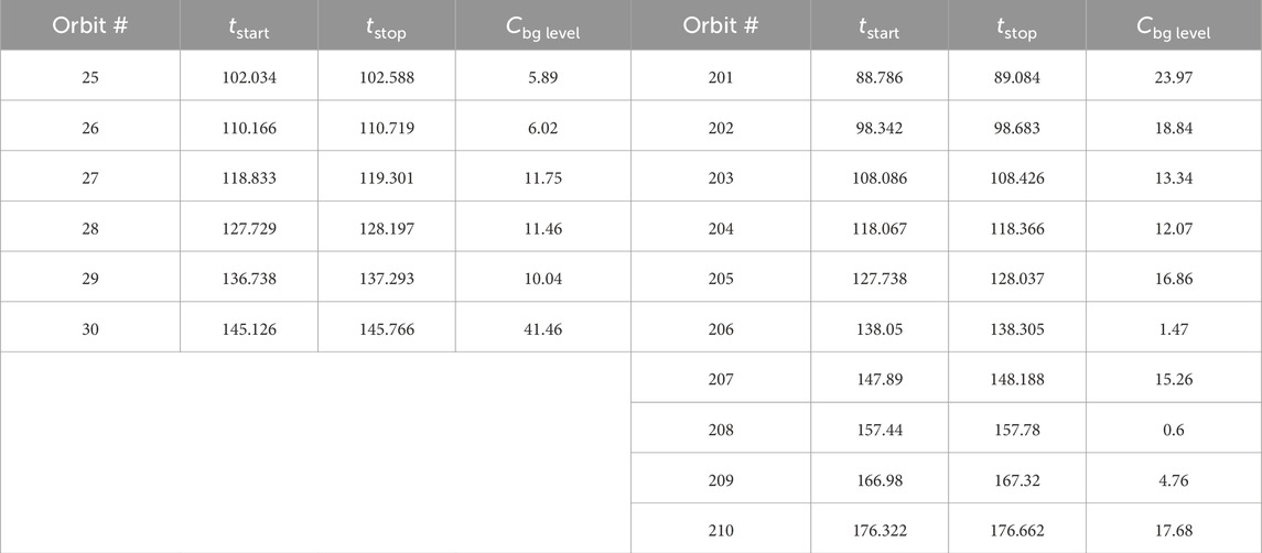
Table 1. Restricted time intervals and the background levels of the outward H fluxes from the plasmasphere.

Note that the background level discussed here is distinct from the background noise described in Section 2.2.1. The background level refers to understanding background counts, potentially originating from the instrument and distributed evenly across the NEP angle. This study uses the accumulated count rates per bin over the entire orbit period rather than the restricted time interval or the period outside the magnetosheath for the following reasons. As seen in Figure 2A, emissions within the magnetosheath (DOY 101.52–102.0) significantly contribute to the total accumulated counts over the entire orbit period. Despite this contribution, the count rate distribution per bin closely resembles that observed during the restricted time interval (see Figure 2C). To minimize contamination from unknown energetic particles, the background level is conservatively accounted for in the analysis and determined from the Gaussian distribution function to fit the accumulated counts per bin over the entire orbit period.

Finally, we consider the spacecraft position of each swath to determine the restricted angle range to ensure the FOV points to the inner exosphere. The restricted angle range changes per orbit since the spacecraft’s position varies above and below the ecliptic plane (Figure 1C). For instance, Figure 2A shows enhanced emissions near 260° during the restricted time interval (DOY 102.034∼102.588) when IBEX was above the ecliptic plane, shifting to ∼285° after DOY 104.4 when IBEX was below the ecliptic plane. The viewing direction (${\theta }_{\text{view}}$) is computed as θ_view = 270°+arctan (z_sc/y_sc), where y_sc and z_sc are the spacecraft’s position components. The restricted angle range is defined as ±9° around the viewing direction (θ_view − 9° to θ_view + 9°), corresponding to the viewing angle bin and two neighboring bins. This angle range allows the IBEX-Lo FOV to cover 4–8 R_E at 25–50 R_E spacecraft distances along the Y_GSE axis, narrowing to 2.6–5.2 R_E if limited to one bin. The red horizontal dashed lines in Figure 2A indicate the restricted angle range. In summary, ENA emissions within the restricted time intervals and angle ranges represent outward H atoms from the inner exosphere.

2.3 The outward H fluxes

We select the 1-h cadence swaths within the restricted time interval for each orbit and then combine the counts in the restricted angle bins (mostly N_bin = 3) for each swath. Since each swath has a cadence start time and spacecraft location vector ($\overrightarrow{r}$), we can produce the total number of counts, $C\left(r\right)$, in the selected angular bins as a function of distance. Then, we calculate the differential fluxes $J_{\mathrm{H}}$ of the outward H atoms at E-step 1 (E_center = 15 eV) for each selected swath as follows:

$J_{\mathrm{H}}\left(r\right)=\frac{\left[\frac{C\left(r\right)}{t_{\text{expo}}\cdot N_{\text{bin}}}-R_{\text{bg}}\right]}{\left(E\cdot G\right)}(2)$

where $t_{\text{expo}}$ is the exposure time, $R_{\text{bg}}$ is the ubiquitous local background H count-rate, E is the center energy of E-step 1, and G is the energy geometric factor. Since a 1-h cadence swath is accumulated over 256 spins, the exposure time ($t_{\text{expo}}$) per 6° angular bin per E-step is computed as (256 spins/8 E-steps) ⋅ (time-per-spin)/(60 angular bins). The ubiquitous local background H count rate $R_{\text{bg}}$ was computed by the IBEX team (Galli et al., 2014; Galli et al., 2017), and it is different from the background level described above. The ubiquitous count rate $R_{\text{bg}}$ depends on energy but is invariant to the observation direction, year, and distance from Earth. The energy geometric factor G, valued at 7.29 × 10⁻⁶ cm² sr, incorporates the sensor ΔE/E, the collimator solid angle FOV, all the efficiencies of transmission through the collimator, internal grid transmission, effects of the spokes that separate each azimuthal quadrant, the energy-dependent conversion efficiency, and TOF efficiency.

3 Results and discussion

In this study, we first investigated the physical properties of outward H fluxes measured by the IBEX-Lo instrument. The outward H fluxes are likely charge-exchange-induced H ENAs produced within the inner exosphere. We analyzed differential H fluxes derived from 35 1-h cadence swaths over 45 days during Case 2009 and 39 1-h cadence swaths over 89 days during Case 2013. Figure 3 illustrates the counts of outward H atoms measured within the restricted NEP angle range for selected 1-h cadence swaths during the restricted time intervals (upper panel), the corresponding signal-to-noise ratios (middle panel), and the differential fluxes of outward H atoms calculated by Equation 2 (bottom panel) as a function of the geocentric radius. For statistical reliability, we excluded fluxes with signal-to-noise ratios below 1.5 in the bottom panel. Additionally, fluxes that measured closer than 28 R_E in 2013 were omitted to avoid possible contamination from magnetosheath ions near the bow shock after our filtration process described in Section 2. Blue squares represent the values from Case 2009, while red circles correspond to values from Case 2013.

Figure 3

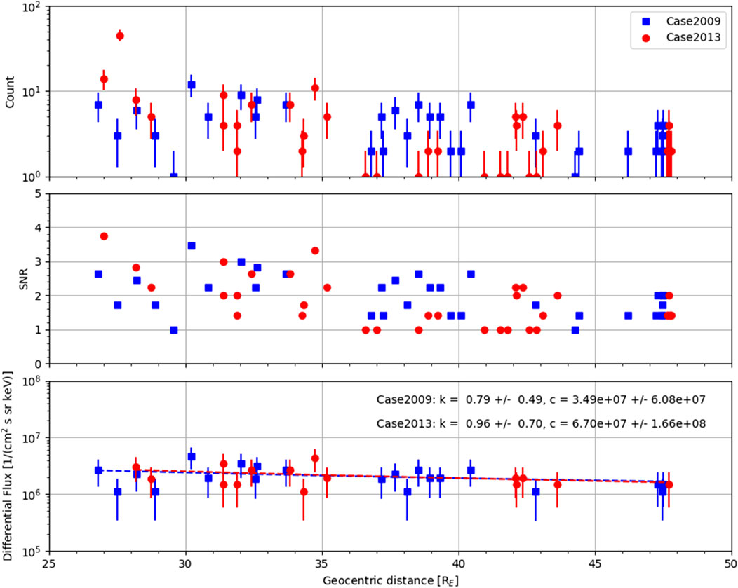
Figure 3. Counts of outward H atoms measured in three angle bins in the restricted angle range on the selected 1-h cadence swaths within the restricted time intervals (upper panel) and the corresponding signal-to-noise ratios (middle panel). The bottom panel shows the computed outward H fluxes as a function of geocentric distance. The power-law fit curves are blue (Case 2009) and red (Case 2013) dashed lines in the bottom panel.

To characterize the physical properties of the outward H fluxes, we applied a power-law function, J = c·r^-k, to fit the measured fluxes. In Figure 3, the dashed lines represent the power-law fits, with power indices k = 0.79 ± 0.49 for Case 2009 (blue) and k = 0.96 ± 0.70 for Case 2013 (red). These power-law fits reveal three key findings. First, the fluxes are on the order of 10⁶ cm⁻² s⁻¹ sr⁻¹ keV⁻¹, as shown in the bottom panel of Figure 3. The average fluxes were (2.10 ± 0.89)×10⁶ cm⁻² s⁻¹ sr⁻¹ keV⁻¹ in 2009 and (2.16 ± 0.87) × 10⁶ cm⁻² s⁻¹ sr⁻¹ keV⁻¹ in 2013. Second, the outward H fluxes gradually decrease with increasing geocentric distance, as indicated by the power indices of 0.79 and 0.96. Although these indices have relatively large uncertainties, their possible range remains positive, confirming that the flux intensity decreases with increasing distance. To further validate this trend, we applied the power-law function to fit the measured fluxes with signal-to-noise ratios above 2.0 and taken within 45 R_E. This yielded positive power indices of 0.73 ± 0.62 for 2009 and 0.88 ± 0.76 for 2013, reinforcing the observed decrease in the flux intensity. Lastly, there is no significant difference in the flux intensities between the 2009 and 2013 spring seasons. Figure 4 shows the F10.7 indices obtained from the OMNIWeb database, where solid lines indicate hourly averages during the 2009 (red) and 2013 (blue) spring seasons. In addition, red squares and blue circles denote the averaged values over the restricted time intervals in the 2009 (red) and 2013 (blue) seasons, respectively. Although the F10.7 indices confirm higher solar radio fluxes in 2013 than in 2009, our results suggest that the outward H fluxes are not influenced by the solar radio flux.

Figure 4

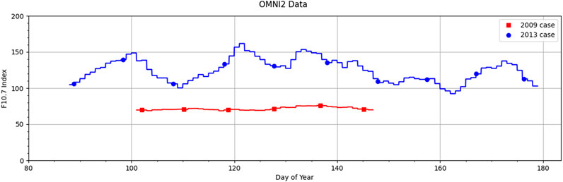
Figure 4. F10.7 indices obtained from the OMNIWeb database: hourly averages are represented as solid lines, and averaged values over the restricted time intervals are shown as red squares (2009 season) and blue circles (2010 season).

To confirm the inner exosphere as the possible source of the outward H fluxes, we consider a simple model for ENAs produced in the inner exosphere. The ENA differential flux ($J_{\text{ENA}}$) at an observer location (${\overrightarrow{r}}_{\text{sc}}$) and the ion differential flux ($J_{\text{ion}}$) are related by the following equation:

$J_{\text{ENA}}\left(E,{\overrightarrow{r}}_{\text{sc}}\right)=\int J_{\text{ion}}\left(E,\overrightarrow{r}\right)\cdot \sigma \left(E\right)\cdot n_{\mathrm{H}}\left(\overrightarrow{r}\right)dr(3)$

where σ(E) is the charge-exchange cross-section, $n_{\mathrm{H}}\left(\overrightarrow{r}\right)$ is the exospheric neutral H density at $\overrightarrow{r}$, and the integral is computed along the LOS crossing the inner exosphere. We simplify this relation under the following assumptions: (1) the ion flux depends only on energy and not on position, i.e., $J_{\text{ion}}\left(E,\overrightarrow{r}\right)=J_{\text{ion}}\left(E\right)$; (2) the exospheric density decreases as $n_{\mathrm{H}}\left(\overrightarrow{r}\right)=n_{\mathrm{H}0}{\left(r_0/r\right)}^3$, where r₀ = 10 R_E; and (3) there is no loss after the ENA is created, i.e., no loss term in Equation 3. Thus, Equation 3 simplifies as follows:

$J_{\text{ENA}}\left(E,{\overrightarrow{r}}_{\text{sc}}\right)=J_{\text{ion}}\left(E\right)\cdot \sigma \left(E\right)\cdot n_{\mathrm{H}0}{r}_0^3\cdot {\displaystyle {\sum }_{\overrightarrow{r}}}\left(r^{-3}\Delta r\right)(4)$

Figure 5A shows the schematic diagram of the simple model for the expected ENA fluxes produced in the inner exosphere. The gray dashed circle represents a sphere with a 4 R_E geocentric radius, the black solid circle indicates the Earth, and the blue dots illustrate example integral points. We consider the situation where the IBEX spacecraft is located along the Y_GSE axis at distances ranging from 25 R_E to 50 R_E. For each location of the IBEX spacecraft, we consider the angle ζ between the Y_GSE axis and an LOS (red solid line in Figure 5A). The restricted angle ζ_lim is defined as the angle at which the LOS passes through the surface of a 1 R_E sphere. We compute the integral along the LOS in the inner exosphere when ζ > ζ_lim, but we perform the integral only in the dawn region when ζ < ζ_lim as the dusk side is blocked by the Earth.

Figure 5

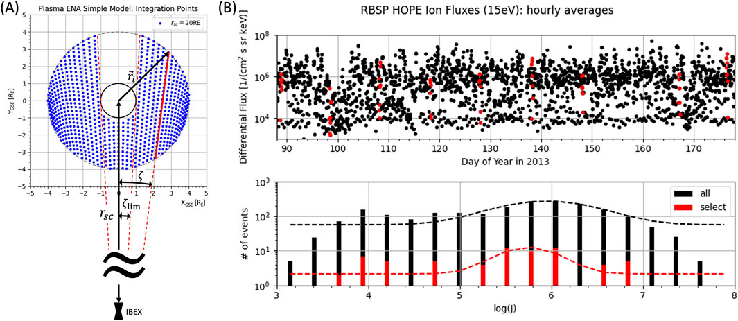
Figure 5. (A) Schematic diagram of the simple model for the expected ENA fluxes produced in the inner exosphere (r < 4 R_E). The dashed circle represents the sphere of 4 R_E geocentric radius, and the blue dots illustrate the integral points. The red solid line is an example LOS inside the inner exosphere. (B) The upper panel shows the ion differential fluxes at 15 eV measured by HOPE/RBSP-A from March 29 to 27 June 2013. The red dots represent the ion fluxes measured in the specific intervals corresponding to the IBEX observation time in Case 2013. The bottom panel shows the distribution of the ion fluxes (black bars for all events, and red bars for the events selected in the restricted time intervals). The dashed lines indicate the Gaussian curves that fit each dataset.

We obtain the 15-eV ion flux from the in situ ion flux observations of the HOPE mass spectrometer aboard the RBSP during the spring season of Case 2013 (days 88–177, 2013). The RBSP was orbiting within a 6 R_E geocentric radius and close to the X_GSE–Y_GSE plane. Figure 5B shows the ion differential fluxes (black dots) at 15 eV, with the red dots representing the ion fluxes measured during the specific intervals corresponding to the restricted time intervals of Case 2013 for the outward H fluxes from the inner exosphere (Table 1). Since the ion fluxes in the restricted time intervals are widely distributed, as seen in the bottom panel of Figure 5B, we compute the mean of the distribution, which corresponds to the center of the peak in the Gaussian function. The red dashed curve represents the fit curve for the ion flux distribution. The mean ion flux is ${\overline{J}}_{\text{ion}}=6.0\times {10}^5$ cm^-2 s⁻¹ sr⁻¹ keV⁻¹ at 15 eV, with one-sigma uncertainties ranging from 2.8 × 10⁵ cm⁻² s⁻¹ sr⁻¹ keV⁻¹ to 1.1 × 10⁶ cm⁻² s⁻¹ sr⁻¹ keV⁻¹, representing the lower and upper limits of the 15 eV ion fluxes. We use the charge-exchange cross-section computed by Lindsay and Stebbings (2005): $\sigma =4.07\times {10}^{-15}$ cm² at E = 15 eV. Finally, we consider the expected ENA fluxes for two cases of the exospheric density at 10 R_E: n_H0 = 10 cm^-3 and 50 cm⁻³ because the neutral density at 10 R_E ranges from 4 to 59 cm⁻³ (Connor et al., 2021).

Figure 6 shows the expected ENA fluxes (green solid line for n_H0 = 10 cm⁻³ and cyan solid line for n_H0 = 50 cm^-3) and the measured outward H fluxes (blue squares for Case 2009 and red circles for Case 2013). The shaded regions represent the uncertainty in the expected ENA fluxes, arising from the lower and upper limits of the ion fluxes. The blue and red dashed lines indicate the power-law fit curves for the measured fluxes. We also computed the power-law fit curves for the expected fluxes, with the estimated power index k = 0.27 ± 0.01. The expected ENA fluxes exhibit two features consistent with the measured outward H fluxes. First, the expected ENA fluxes slightly decrease as the geocentric distance increases. This decrease in the intensity is reasonable because the LOS length in the sphere of 4 R_E varies depending on the spacecraft’s location. When the spacecraft is closer to Earth, the LOS slopes are slightly steeper than when the spacecraft is further away. The steeper slope causes longer integral distances in the sphere of 4 R_E and increases the probability of ENA production. Second, the upper limit of the expected ENA fluxes of n_H0 = 50 cm^-3 is of the same order of magnitude as the measured outward H fluxes. This suggests that the measured outward H fluxes may include ENAs generated in the inner exosphere.

Figure 6

Figure 6. Differential fluxes of the outward H ENAs as a function of the geometric distance. The blue squares and red circles represent the outward H ENA fluxes measured by IBEX in 2009 and 2013, respectively. The blue and red dashed lines indicate the power-law fit curves for each measured flux. The green and cyan solid lines represent the expected H ENA fluxes with n_H0 = 10 cm⁻³ and 50 cm⁻³, respectively. The shadows represent the uncertainty of the expected ENA fluxes.

The discrepancy between the observed and expected H ENAs may arise from the simplicity of our model. We assumed that the ion flux does not depend on location, that the exospheric density decreases as 1/r³, and that the ENAs are created in the sphere of 4 R_E. However, the ion flux exhibits large variability in magnitude, as seen in the bottom panel of Figure 5B, and the exospheric density does not exactly follow the inverse cube law in the inner exosphere. The IBEX-Lo FOV covers a larger sphere than the inner exosphere when the spacecraft was further than 25 R_E geocentric distance. Furthermore, we only used the ion flux measurements from the 2013 season as no 15 eV ion flux observations were available for the 2009 season. As a result, the expected ENA fluxes calculated by the simple model did not fully capture the ENAs produced during the solar minimum. On the other hand, the measured outward H fluxes could be overestimated due to contamination by any energetic particles even though we removed most of the contaminating sources. Despite these limitations, the two features described above support the conclusion that the measured outward H fluxes are closely related to the ENAs produced in the inner exosphere.

There are various plasma populations in the terrestrial magnetosphere. The protons of plasmasphere origin are at a temperature of approximately 2,000–10,000 K (0.1 to a few eV), whereas exospheric H is at approximately 750–1,250 K (Shizgal and Arkos, 1996). The combination of polar wind flow and a centrifugal acceleration can give the ions energies above 10 eV, which can send them back into the magnetotail (lobal wind, 10–300 eV). In the magnetotail, the curvature drift across the tail through the cross-tail potential can add energies of 1 keV and more (plasma sheet, 0.5–5 keV) (Chappell et al., 2008). The amount of energy gained by these particles of plasmasphere origin and the resulting flow paths can lead to two separate plasma populations: the warm plasma cloak and the ring current. The warm plasma cloak is a bidirectional, field-aligned distribution of ions with an energy range of a few eV to hundreds of eV. Ions with these characteristics are found outside the plasmasphere across the night side and can extend eastward from the plasmapause to the magnetopause. The ring current is composed of more accelerated ions with an energy range of 3–30 keV that moves westward by the curvature drifts. These magnetospheric plasma populations can become charge-exchange-induced ENAs, which could be measured by the IBEX-Lo instrument. In this study, we found that the outward H fluxes measured by the IBEX-Lo are closely associated with the charge-exchange-induced H ENAs. Since these plasma populations have different dynamics and behaviors, we anticipate that the observations of outward H fluxes show temporal and spatial evolutions depending on an observation season and a side-viewing vantage point if they contain the terrestrial ENAs. Because the full energy range of the IBEX-Lo instrument overlaps with the energy ranges of the magnetospheric plasma populations, we anticipate that the energy-resolved ENA observations of IBEX-Lo could show different energy spectra depending on what the instrument observed. We plan to continue researching the dynamics and energy spectra of the outward H fluxes as follow-up projects.

4 Summary

In this study, we first investigated the IBEX-Lo 15 eV ENA observations when the inner exosphere entered the IBEX FOV during two spring seasons: 11 April–26 May 2009 (Orbit 25–30, DOY 101–146) and 29 March–27 June 2013 (Orbit 201–210, DOY 88–178). We used the ENA histogram data obtained from the IBEX Raw Data Release (https://ibex.princeton.edu) and defined the restricted time intervals and angle ranges where the H fluxes escaping from the inner exosphere (<4 R_E) could be detected by the IBEX-Lo instrument. Then, we estimated the outward H fluxes in the outer exosphere (25 ∼ 50 R_E). The measured outward H fluxes are characterized by three key findings: (1) the fluxes vary in the order of 10⁶ cm⁻² s⁻¹ sr⁻¹ keV⁻¹, (2) the outward H fluxes gradually decrease with increasing geocentric distance, and (3) there is no significant difference in flux intensities between the 2009 and 2013 spring seasons.

Additionally, we computed the expected H ENA fluxes produced in the inner exosphere by solving Equation 4 using ion flux data from HOPE on RBSP and a simplified exospheric density model inversely proportional to the cube of the geocentric distance. In this calculation, we assume that the ion flux depends only on energy and not on position as well as there is no loss after the ENA is created. Both the measured outward H fluxes and the expected ENA fluxes reveal two similar features: (a) a slight decrease in the intensity with increasing geocentric distance and (b) intensities on the order of 10⁶ cm⁻² s⁻¹ sr⁻¹ keV⁻¹. These two features strongly suggest that the observed outward H fluxes are associated with the H ENAs produced in the inner exosphere. We also found no significant difference in the intensities of the outward H fluxes measured in different solar radio flux conditions (quiet in 2009 versus more active in 2013). However, further statistical analysis is required to fully understand the variation of outward H fluxes over the solar cycle, which is left for future work.

Data availability statement

Publicly available datasets were analyzed in this study. These data can be found here: https://ibex.princeton.edu.

Author contributions

JP: Conceptualization, Data curation, Formal Analysis, Funding acquisition, Investigation, Methodology, Visualization, Writing–original draft, Writing–review and editing. HC: Funding acquisition, Writing–review and editing.

Funding

The author(s) declare that financial support was received for the research and/or publication of this article. This research was supported by the NASA Goddard Space Flight Center through Cooperative Agreement 80NSSC21M0180 to the University of Maryland Baltimore County, Partnership for Heliophysics and Space Environment Research (PHaSER), and the NASA Heliophysics Theory, Modeling, and Simulation (H-TMS) program.

Acknowledgments

The authors thank the IBEX team (PI Dave McComas) for making this work possible. The authors thank Adam Szabo, Nikolaos Paschalidis, and Jaewoong Jung for their support. The authors also acknowledge the International Space Science Institute on the ISSI team titled “The Earth’s Exosphere and its Response to Space Weather.” The authors thank the topical editor and the referees for the discussions and for their extensive help in improving the paper.

Conflict of interest

The authors declare that the research was conducted in the absence of any commercial or financial relationships that could be construed as a potential conflict of interest.

Generative AI statement

The author(s) declare that no generative AI was used in the creation of this manuscript.

Publisher’s note

All claims expressed in this article are solely those of the authors and do not necessarily represent those of their affiliated organizations, or those of the publisher, the editors and the reviewers. Any product that may be evaluated in this article, or claim that may be made by its manufacturer, is not guaranteed or endorsed by the publisher.

References

Bzowski, M., Kubiak, M. A., Moebius, E., Bochsler, P., Leonard, T., Heirtzler, D., et al. (2012). Neutral interstellar Helium parameters based on IBEX-lo observations and test particle calculations. ApJS 198, 12. doi:10.1088/0067-0049/198/2/12

CrossRef Full Text | Google Scholar

Chappell, C. R., Huddleston, M. M., Moore, T. E., Giles, B. L., and Delcourt, D. C. (2008). Observations of the warm plasma cloak and an explanation of its formation in the magnetosphere. J. Geophys. Res. 113, A09206. doi:10.1029/2007JA012945

CrossRef Full Text | Google Scholar

Connor, H. K., Sibeck, D. G., Collier, M. R., Baliukin, I. I., Branduardi-Raymont, G., Brandt, P. C., et al. (2021). Soft X-ray and ENA imaging of the Earth’s dayside magnetosphere. J. Geophys. Res. 126, e2020JA028816. doi:10.1029/2020JA028816

PubMed Abstract | CrossRef Full Text | Google Scholar

Dayeh, M. A., Fuselier, S. A., Funsten, H. O., McComas, D. J., Ogasawara, K., Petrinec, N. A., et al. (2015). Shape of the terrestrial plasma sheet in the near-Earth magnetospheric tail as imaged by the Interstellar Boundary Explorer. Geophys. Res. Lett. 42, 2115–2122. doi:10.1002/2015GL063682

CrossRef Full Text | Google Scholar

Dayeh, M. A., Szalay, J. R., Ogasawara, K., Fuselier, S. A., McComas, D. J., Funsten, H. O., et al. (2020). First global images of ion energization in the terrestrial foreshock by the interstellar boundary explorer. GRL 47, e2020GL088188. doi:10.1029/2020GL088188

PubMed Abstract | CrossRef Full Text | Google Scholar

Funsten, H. O., Allegrini, F., Bochsler, P., Dunn, G., Ellis, S., Everett, D., et al. (2009). The Interstellar Boundary Explorer high energy (IBEX-Hi) neutral atom imager. Space Sci. Rev. 146, 75–103. doi:10.1007/s11214-009-9504-y

CrossRef Full Text | Google Scholar

Fuselier, S. A., Bochsler, P., Chornay, D., Clark, G., Crew, G. B., Dunn, G., et al. (2009). The IBEX-Lo sensor. Space Sci. Rev. 146, 117–147. doi:10.1007/s11214-009-9495-8

CrossRef Full Text | Google Scholar

Fuselier, S. A., Dayeh, M. A., Galli, A., Funsten, H. O., Schwadron, N. A., Petrinec, S. M., et al. (2020). Neutral atom imaging of the solar wind-magnetosphere-exosphere interaction near the subsolar magnetopause. Geophys. Res. Lett. 47, e2020GL089362. doi:10.1029/2020GL089362

PubMed Abstract | CrossRef Full Text | Google Scholar

Fuselier, S. A., Dayeh, M. A., Livadiotis, G., McComas, D. J., Ogasawara, K., Valek, P., et al. (2015). Imaging the development of the cold dense plasma sheet. Res. Lett. 42, 7867–7873. doi:10.1002/2015GL065716

CrossRef Full Text | Google Scholar

Fuselier, S. A., Funsten, H. O., Heirtzler, D., Janzen, P., Kucharek, H., McComas, D. J., et al. (2010). Energetic neutral atoms from the Earth’s subsolar magnetopause. Geophys. Res. Lett. 37, L13101. doi:10.1029/2010GL044140

CrossRef Full Text | Google Scholar

Galli, A., Wurz, P., Fuselier, S. A., McComas, D. J., Bzowski, M., Sokol, J. M., et al. (2014). Imaging the heliosphere using neutral atoms from solar wind energy down to 15 eV. ApJ 796, 9. doi:10.1088/0004-637X/796/1/9

CrossRef Full Text | Google Scholar

Galli, A., Wurz, P., Schwadron, N. A., Kucharek, H., Moebius, E., Bzowski, M., et al. (2017). The downwind hemisphere of the heliosphere: eight years of IBEX-Lo observations. ApJ 851, 2. doi:10.3847/1538-4357/aa988f

CrossRef Full Text | Google Scholar

Hart, S. T., Dayeh, M. A., Reisenfeld, D. B., Janzen, P. H., McComas, D. J., Allegrini, F., et al. (2021). Probing the magnetosheath boundaries using Interstellar Boundary Explorer (IBEX) orbital encounters. J. Geophys. Res. 126, e2021JA029278. doi:10.1029/2021JA029278

PubMed Abstract | CrossRef Full Text | Google Scholar

Jerab, M., Nemecek, Z., Safrankova, J., Jelinek, K., and Merka, J. (2004). Improved bow shock model with dependence on the IMF strength. Planet. Space Sci. 53, 85–93. doi:10.1016/j.pss.2004.09.032

CrossRef Full Text | Google Scholar

Lindsay, B. G., and Stebbings, R. F. (2005). Charge transfer cross sections for energetic neutral atom data analysis. J. Geophys. Res. 110, A12213. doi:10.1029/2005JA011298

CrossRef Full Text | Google Scholar

McComas, D. J., Allegrini, F., Bochsler, P., Bzowski, M., Collier, M., Fahr, H., et al. (2009). IBEX-interstellar boundary explorer. Space Sci. Rev. 146, 11–33. doi:10.1007/s11214-009-9499-4

CrossRef Full Text | Google Scholar

McComas, D. J., Dayeh, M. A., Allegrini, F., Bzowski, M., DeMajistre, R., Fujiki, K., et al. (2012). The first three years of IBEX observations and our evolving heliosphere. ApJS 203, 1. doi:10.1088/0067-0049/203/1/1

CrossRef Full Text | Google Scholar

McComas, D. J., Dayeh, M. A., Funsten, H. O., Fuselier, S. A., Goldstein, J., Jahn, J.-M., et al. (2011). First IBEX observations of the terrestrial plasma sheet and a possible disconnection event. J. Geophys. Res. 116, A02211. doi:10.1029/2010JA016138

CrossRef Full Text | Google Scholar

Moebius, E., Bochsler, P., Bzowski, M., Crew, G. B., Funsten, H. O., Fuselier, S. A., et al. (2009). Direct observations of interstellar H, He, and O by the interstellar boundary explorer. Science 326, 969–971. doi:10.1126/science.1180971

CrossRef Full Text | Google Scholar

Ogasawara, K., Angelopoulos, V., Dayeh, M. A., Fuselier, S. A., Livadiotis, G., McComas, D. J., et al. (2013). Characterizing the dayside magnetosheath using energetic neutral atoms: IBEX and THEMIS observations. J. Geophys. Res. 118, 3126–3137. doi:10.1002/jgra.50353

CrossRef Full Text | Google Scholar

Petrinec, S. M., Dayeh, M. A., Funsten, H. O., Fuselier, S. A., Heirtzler, D., Janzen, P., et al. (2011). Neutral atom imaging of the magnetospheric cusps. J. Geophys. Res. 116, A07203. doi:10.1029/2010JA016357

CrossRef Full Text | Google Scholar

Shizgal, B. D., and Arkos, G. G. (1996). Nonthermal escape of the atmospheres of venus, Earth, and mars. Rev. Geophys. 34, 483–505. doi:10.1029/96RG02213

CrossRef Full Text | Google Scholar

Shue, J. H., Song, P., Russell, C. T., Steinberg, J. T., Chao, J. K., Zastenker, G., et al. (1998). Magnetopause location under extreme solar wind conditions, J. Geophys. Res., 103, 17,17691–17700. doi:10.1029/98JA01103

CrossRef Full Text | Google Scholar

Vugrin, K. W., Swiler, L. P., Roberts, R. M., Stucky-Mack, N. J., and Sullivan, S. P. (2007). Confidence region estimation techniques for nonlinear regression in groundwater flow: three case studies. Water Resour. Res. 43, W03423. doi:10.1029/2005WR004804

CrossRef Full Text | Google Scholar

Wurz, P., Fuselier, S. A., Moebius, E., Funsten, H. O., Brandt, P. C., Allegrini, F., et al. (2009). IBEX backgrounds and signal-to-noise ratio. SSR 146, 173–206. doi:10.1007/978-1-4419-1448-4_9

CrossRef Full Text | Google Scholar