An open source code for modeling radio wave propagation in earth’s ionosphere

We present FARR (Finite-difference time-domain ARRay), an open source, high-performance, finite-difference time-domain (FDTD) code. FARR is specifically designed for modeling radio wave propagation in collisional, magnetized plasmas like those found in the Earth’s ionosphere. The FDTD method directly solves Maxwell’s equations and captures all features of electromagnetic propagation, including the effects of polarization and finite-bandwidth wave packets. By solving for all vector field quantities, the code can work in regimes where geometric optics is not applicable. FARR is able to model the complex interaction of electromagnetic waves with multi-scale ionospheric irregularities, capturing the effects of scintillation caused by both refractive and diffractive processes. In this paper, we provide a thorough description of the design and features of FARR. We also highlight specific use cases for future work, including coupling to external models for ionospheric densities, quantifying HF/VHF scintillation, and simulating radar backscatter. The code is validated by comparing the simulated wave amplitudes in a slowly changing, magnetized plasma to the predicted amplitudes using the WKB approximation. This test shows good agreement between FARR and the cold plasma dispersion relations for O, X, R, and L modes, while also highlighting key differences from working in the time-domain. Finally, we conclude by comparing the propagation path of an HF pulse reflecting from the bottomside ionosphere. This path compares well to ray tracing simulations, and demonstrates the code’s ability to address realistic ionospheric propagation problems.

1 Introduction

The Finite-Difference Time-Domain (FDTD) method directly solves the full vector form of Maxwell’s equations in a medium (Yee, 1966). It is an extremely powerful, fully explicit method used across a variety of industries and applications such as electronics, antenna design, and radiology (Taflove and Hagnes, 2005). The ability to model inhomogeneous media and realistic waveforms makes the FDTD method an ideal tool for modeling radio wave propagation through the ionosphere. In this work, we present initial results from the newly developed, open source FARR (Finite-difference time-domain ARRay) code and its applications to radio wave propagation.

The Earth’s ionosphere can have dramatic effects on radio waves propagating through the ionosphere. HF (3–30 MHz) signals will refract when the local plasma frequency is near the transmitted wave’s frequency, causing a bending of the direction of propagation or even reflection when the plasma frequency is higher than the wave frequency. Instabilities and structures in the ionosphere will also create localized irregularities in the plasma density that can affect and degrade radio waves from HF to L-band (1–2 GHz) ranges. The phase and amplitude scintillation of L-band signals from GPS and GNSS satellites is a prominent example of space weather effects on modern technology (Coster and Komjathy, 2008).

The size of ionospheric irregularities compared to the Fresnel length determines if radio wave scintillation is driven primarily by refraction (bending of ray paths) or by diffraction (interference patterns around an obstacle). In the high-latitude ionosphere the gradient-drift instability creates kilometer scale irregularities that are observationally linked to L-band scintillation (Mrak et al., 2018). The Fresnel length for trans-ionospheric L-band signals is between 200–500 m (Loucks et al., 2017), and therefore the scintillation from the gradient-drift instability is primarily a refractive phenomenon. However, in the E-region, the gradient-drift instability also drives a secondary Farley-Buneman instability that produces irregularities at scales as small as a few meters, well below the Fresnel length (Young et al., 2019; Young et al., 2017; Young et al., 2020). The need to model both refractive and diffractive scintillation effects from multi-scale density structures is the motivation for developing the FARR code.

Modeling wave propagation through multi-scale ionospheric irregularities with the FDTD method has several advantages over codes that work in the geometric optics limit. The FDTD method is a full-wave solution that is distinct from raytracing and does not rely on the geometric optics assumption, and therefore naturally models both refraction and diffraction. By working in the time domain, the FDTD method is able to model realistic time domain wave sources with finite bandwidths. The simulation domain can include complex 3D structures with a variety of inhomogeneous material properties as either a boundary (e.g., reflecting conductor), a change in the dielectric material, or a plasma (via the continuity equation for current density $\vec{J}$). Additionally, magneto-ionic effects such as differential mode delay and Faraday rotation result from the inclusion of a magnetized plasma in the FDTD domain.

While the FDTD method has long been popular in many fields, in recent years there has been a focus on developing computationally efficient algorithms for anisotropic media, including magnetized plasmas (Yu and Simpson, 2010; Samimi and Simpson, 2015; Pokhrel et al., 2018). These algorithms have enabled the development of versatile FDTD simulations that can study global ELF waves (Yu et al., 2012) or localized HF propagation in the ionosphere (Smith et al., 2020a; Smith et al., 2020b). Despite recent advances in this area, there is no open access tool for performing FDTD simulations in a magnetized collisional plasmas. To facilitate new studies of electromagnetic wave propagation in the ionosphere, we have created a new open source Finite-Difference Time-Domain code.

The overall purpose of this paper is to provide a thorough description of the major features found in FARR and to show simulation results highlighting these features. We provide a short discussion of the computational design of FARR in Section 2.1, including performance metrics. Section 2.2 discusses the different boundary conditions in FARR including reflecting, periodic, and absorbing. The method used to include the effects of an inhomogeneous plasma is detailed in Section 2.4. FARR also includes a Total-Field Scattered-Field (TFSF) formulation that is used for introducing plane wave sources and studying scattering processes. Section 2.3 provides an overview of the TFSF domain and shows typical use cases. Validation of the code and its initial results for a few ionospheric propagation problems are shown in Section 3, and further applications are discussed in Section 4.

2 FARR finite-difference time-domain code

2.1 Overview

FARR (Finite-difference time-domain ARRay) is a new high-performance 3D FDTD code designed for studying electromagnetic wave propagation in a magnetized collisional plasma. It is developed in C++ code optimized for studying computationally intensive problems. FARR is an open access project that is designed to be easily installed and used on a wide range of systems; from personal computers to supercomputers. To take advantage of highly parallel systems like next-generation supercomputers, FARR is domain decomposed and parallelized in three dimensions using Message Passing Interface (MPI). All I/O operations are handled using the ADIOS2 library (Godoy et al., 2020), and files are stored using either Binary Pack (BP) or HDF5 format. Figure 1 demonstrates strong scaling for FARR, running with up to 2048 processors on the Frontera system at the Texas Advanced Computing Center. Writing all vector quantities of $\vec{E}$ and $\vec{B}$ to disk can be time consuming, so custom I/O is available using the provided field monitor class, which defines a series of locations in the grid to save for later analysis.

Figure 1

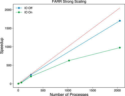
Figure 1. Strong scaling for FARR using a computational domain size of 512 × 1024 × 1024, showing the number of processors vs. speedup. We perform this test for the case of a magnetized, collisional plasma, and check the scaling with all I/O turned on (green curve) vs. all I/O turned off (blue curve). The dashed line shows the theoretical best case speedup.

FARR and its user manual can be easily accessed from its GitLab page at https://gitlab.com/longleywj/farr/. The fastest way to install FARR is using Conda to gather all requirements, which is detailed in the documentation. However, when using FARR for very large scale simulations, it can be beneficial to build against any prebuilt libraries/modules that are available. Post-processing of runs is handled through several easy and robust Python routines, including a lightweight class designed to interface with the output BP/HDF5 files. For complex 3D simulations, visualization through Paraview is available using either BP the files or a custom HDF5 loader.

FARR has a rich set of features that allow it to be configured to study a variety of different problems. The core FDTD algorithm that FARR uses is shown in Figure 2. In the rest of this section, we will provide a brief overview and accompanying examples of the key features that exist in FARR.

Figure 2

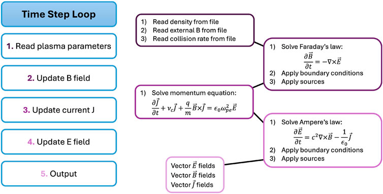
Figure 2. Block diagram of the core time step loop in FARR.

2.2 Boundary conditions

FARR currently has three different boundary conditions (BCs) implemented: reflecting, periodic, and a perfectly matched layer (PML) that absorbs all incident waves. We implement boundary conditions independently for each axis. For example, a user may wish to run with periodic BCs in the x and y directions and a PML in the z direction. This is easily set by flags in the input deck when running FARR.

Without explicit boundary conditions, the grid of an FDTD code is terminated by perfectly electrically conductive (PEC) boundary conditions that reflect all outwardly moving electromagnetic waves. This boundary condition is an unrealistic restriction in most cases and has pushed the development of more advanced absorbing boundary conditions which can dramatically lower the amount of energy reflected at the edges of the computational domain. The current state-of-the-art absorbing boundary condition is known as the perfectly matched layer (PML). The PML acts as a nonphysical lossy medium which exponentially decays outgoing waves.

In FARR we implement the convolutional, stretched-coordinate form of the PML, which is designed to be computationally efficient and independent of the material being simulated (Roden and Gedney, 2000). Figure 3 shows how the PML absorbs all incident waves from a point source at different times. This form of PML can handle inhomogenous, dispersive, anisotropic and nonlinear media. However, the perfectly matched layer has been shown to be unstable under certain conditions. When incident upon the PML, if the wave group and phase velocity contain anti parallel components, the wave will instead grow exponentially (Bécache et al., 2003). This situation can arise when simulating plane waves in a magnetized plasma (Chevalier et al., 2008), and it is partially for this reason that we choose to implement the Total-Field Scattered-Field formulation in FARR (Section 2.3).

Figure 3

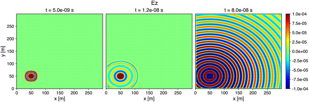
Figure 3. Z component of the electric field at early, middle and late times of a simulation. Here we simulate a $\widehat{z}$ polarized sine wave source, with a 3 × 3 domain decomposition. The perfectly matched layer boundary condition absorbs all outward moving waves, regardless of the angle of incidence.

2.3 Total-field scattered-field formulation

In FDTD simulations it is often useful to make a distinction between the source wave field and any scattering, reflection, etc. that occurs as a result of the problem being simulated. The total-field scattered-field (TFSF) formulation is a boundary condition that is interior to and in addition to the BCs in Section 2.2. It is designed to separate the FDTD space into two distinct regions: the total-field and scattered-field regions, in which the normal FDTD algorithm is applied normally within each separate region (Merewether et al., 1980). At the boundary of these two regions, a correction term is included for the electric and magnetic field components, which will act as a source for the total field region. The wave source is analytically subtracted off at the TFSF boundary using the matched numerical dispersion technique of Guiffaut and Mahdjoubi (2000). The source wave will not enter the scattered field region unless it has been distorted/scattered in some way. In this way, we can implement arbitrary sources and distinguish them from the scattering processes that result from the simulation. For an in depth discussion of the total-field scattered formulation see Taflove and Hagnes (2005).

The TFSF is an integral part of FARR for several reasons, the most important of which is for introducing sources into the FDTD grid. Other methods for sources, such as hard sources, can cause spurious reflections and limit the practical uses of FDTD simulations (Taflove and Hagnes, 2005). FARR is designed to study ionospheric and radio science problems where we can assume the region of interest is in the far-field of any sources, and therefore we need to be able to model plane wave sources accurately. This creates an issue as plane wave sources are not directly compatible with the absorbing PML as the edges of the wavefront will drag through the PML and distort the wavefront or even cause a shift in the phase direction leading to the instability discussed in Section 2.2. The TFSF acts as an internal boundary condition that removes the source field before terminating the grid with the perfectly matched layer. Figure 4 shows how these two boundary conditions are applied in succession.

Figure 4

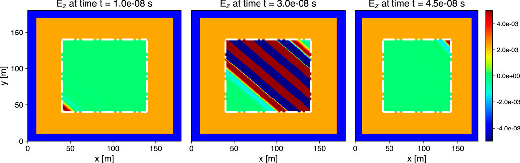
Figure 4. Schematic of the FARR computational domain showing the PML region (blue), free space region (orange) and main computational domain (inside dashed line). At the TFSF boundary, we introduce a sinusoidally modulated Gaussian pulse propagating at a 45$°$ angle. Here, because we simulate free space in the entire domain, the wave remains unchanged and, as expected, does not exit the TFSF region.

2.4 Magnetized collisional plasmas

FARR is designed to study electromagnetic wave propagation in collisional plasmas like Earth’s ionosphere. To implement plasma effects, we must solve the electron momentum equation at each time step for the current $\vec{J}$. In finite-difference form, the momentum is given by Equation 1:

$\frac{{\vec{J}}^{n+1/2}-{\vec{J}}^{n-1/2}}{\mathrm{\Delta }{t}_c}+{\nu }_e{\vec{J}}^{n-1/2}={ϵ}_0{\omega }_{pe}^2\vec{E}-{\vec{\omega }}_{ce}\times \left(\frac{{\vec{J}}^{n+1/2}+{\vec{J}}^{n-1/2}}{2}\right)(1)$

where $\mathrm{\Delta }{t}_c$ is the time step required for stability of the plasma routine given the local plasma $({\omega }_{pe})$, collision $({\nu }_e)$, and cyclotron frequencies $({\omega }_{ce})$. This equation can be applied for each relevant species, however, over the short timescales of FARR simulations, we assume only electron motion is important. To solve for $J^{n+1/2}$, we use the method described by Samimi and Simpson (2015), which is fully explicit and computationally efficient. However, when $\mathrm{\Delta }{t}_c$ is substantially lower than the simulation time step $\mathrm{\Delta }t$ (required to satisfy the Courant-Friedrichs-Lewy condition), the current must to be updated multiple times before use in the main FDTD algorithm. This case typically occurs when the collision rate is high, and therefore the collisional routine from Pokhrel et al. (2018) is also implemented. This routine requires solving matrix equations, but can update the current density with only one step. All matrix updates are solved using the linear algebra library Armadillo (Sanderson and Curtin, 2019).

When running simulations in FARR, the proper algorithm and time step are selected automatically according to the global plasma, collision and cyclotron frequencies. As mentioned in Section 2.2, when simulating magnetized plasmas, the perfectly matched layer boundary condition can become unstable. In this case, to prevent instability, we recommend simulating with either periodic or reflecting boundary conditions, grading the plasma density to 0 at the boundaries, or containing the plasma within the total-field scattered-field domain (see Section 2.3).

There are several options for running a simulation with a background plasma in FARR. A global background magnetic field, plasma frequency and collision frequency can be specified in the input deck. FARR can also read spatially varying collision and plasma frequencies from an external HDF5 file that aligns with either the TFSF region or the entire simulation domain. Optionally, for studying time scales over which temporal variation of the plasma becomes important, the HDF5 file can contain a series of time steps to update the background plasma over the simulation. The best way to create an external HDF5 file for FARR is through the customizable Python adapter that reads in plasma densities from the HDF5 file and transforms the density to FARR’s grid. An example is provided in the source code to generate an HDF5 file from the output of an Electrostatic Parallel Particle-In-Cell (EPPIC) (Oppenheim and Dimant, 2004) simulation. This routine can be readily modified to read in plasma densities from other plasma simulators.

2.5 Near to far field transformation

FARR includes a time domain near-to-far field transformation (NTFF) as part of the Python post-processing suite. The NTFF is based on the Surface Equivalence Principle, which holds that if the electric current, $\vec{J}$, and magnetic current, $\vec{M}$, are known everywhere on a closed surface, and there are no sources external to the surface, the complex amplitude anywhere outside the surface can be determined. Typical use cases for the near to far field transformation in FDTD include determining far field radiation patterns of antennas and measuring scattering cross sections.

In practice, this allows one to define a surface inside the FARR simulation and use it to compute the time varying electric and magnetic fields anywhere outside the computational domain. We use the method of Luebbers et al. (1991) to determine the time domain electromagnetic response at an arbitrary location in space. For the NTFF to be valid and work in FARR, all components of the electric and magnetic field on a closed surface must be output, and the surface should be defined to encompass all sources and scatterers. To perform the NTFF, we first define the closed surface to pass through $E_z$ nodes in the grid. We then linearly interpolate $\vec{E}$ and $\vec{H}$ to the surface, and determine the surface electric $(\overrightarrow{j_s}=\widehat{n}\times \overrightarrow{H_s})$ and magnetic $(\overrightarrow{m_s}=-\widehat{n}\times \overrightarrow{E_s})$ currents, where $\widehat{n}$ is the surface outward normal on surface $s$. Integration and scaling of the surface currents (see Luebbers et al., 1991) yields the appropriate far field response. In Figure 5 we simulate a half-wave dipole antenna transmitting a 15 MHz sine wave. The electric and magnetic fields are post-processed using the NTFF routine to determine the far field radiation pattern 60 km outside of the computational domain, which is in good agreement with the theoretical pattern.

Figure 5

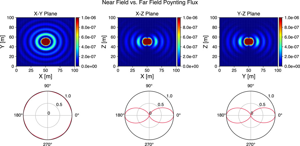
Figure 5. Near to far field transformation for the case of a simple half-wave dipole antenna. The top row shows the Poynting flux in the simulation domain’s X-Y, X-Z and Y-Z planes. The bottom row shows the normalized far field radiation patterns at distances of 6 km away from dipole antenna. The simulated far field patterns (red) agree well with the theoretical far field radiation pattern.

2.6 Antenna elements and arrays

When the regions of interest for an FDTD simulation are in the near field, or when spatially varying waveforms are required, the total-field scattered-field can no longer be used as a source. Under these conditions we introduce two additional sources, individual antenna elements and antenna arrays. Elements and arrays are applied to the simulation domain with individual locations, phases and gains, giving the user complete control over the transmission pattern. Individual antenna elements are created within FARR using the thin-wire approximation (Umashankar et al., 1987), which allows for computationally efficient and accurate modeling of sub-cell features. This type of source is particularly useful when studying high frequency (HF) radio propagation in the bottomside ionosphere.

To demonstrate the use of antenna elements and phased arrays in FARR, we simulate arrays of half-wave dipole antennas operating at 10 MHz. The arrays have 2, 4 and 8 colinear elements, and are phased to have the main lobe at 90$°$ (vertical) or 45$°$ (oblique) elevation angles. The far field radiation patterns are determined using the near to far field transform (Section 2.5) and the results are shown in Figure 6. FARR includes Python routines to aid in setting the location and phasing of any number of antenna elements. When simulating arrays, all antenna elements use the same transmission with user specified phase offsets. For complete control over phase, location, transmission, etc., individual antenna elements should be used.

Figure 6

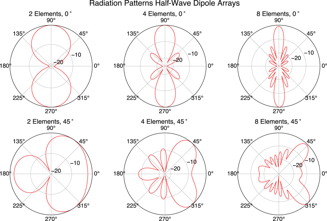
Figure 6. Normalized far field radiation patterns for 2, 4, and 8 element half-wave dipole antenna arrays, with both vertical and oblique (45$°$) incidence. Radiation patterns are determined a radius of 1 km from the center of the phased array using the near to far field transform.

3 Results

3.1 Dispersive effects in a plasma

A key feature of FARR is the ability propagate waves through an inhomogeneous, magnetized plasma. To validate the plasma routines in 2.4, we run a set of simulations with a slowly varying plasma density and compare the results to the dispersion relations for O, X, R, and L mode waves. We perform these simulations in both collisionless and weakly collisional regimes to validate all routines. Table 1 shows the simulation parameters for FARR. The plasma density is set to increase linearly from 0 to $n_{\mathit{max}}\approx 1.24\times 10^{12}{m}^{-3}$ over 2,000 m. The amplitude of an electromagnetic wave in a slowly varying plasma is described by the WKB approximation (Bellan, 2006). The WKB solution is a complex exponential, where the amplitude and phase change slowly as the wave propagates:

$E_1\left(x\right)=\frac{1}{\sqrt{k_x\left(x\right)}}\exp \left(i{\int }_0^x{k}_x\left(x^{\prime }\right)d{x}^{\prime }\right)(2)$

Table 1

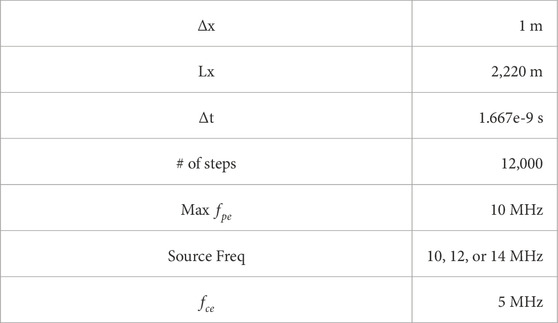
Table 1. FARR simulation parameters for WKB validation. The y and z directions are periodic, and the x direction imposes the source wave using the TFSF method. The magnetic field is oriented in the z-direction for O and X mode tests, and oriented in the x-direction for R and L mode tests.

In Equation 2, the amplitude and phase are determined by the wavenumber in the direction of the inhomogeneity; chosen as the x-direction here. For an O-mode wave, the wavenumber will vary spatially as the plasma frequency ${\omega }_{pe}(x)$ varies, via the dispersion relation given in Equation 3:

$k_x^2\left(x\right)=\frac{{\omega }^2}{c^2}\left(1-\frac{{\omega }_{pe}^2\left(x\right)}{{\omega }^2}\right)-k_y^2-k_z^2(3)$

The simulations will propagate waves in the x-direction, so $k_y=k_z=0$. Therefore, as the wave propagates through the plasma, its amplitude at each position is a direct validation of the dispersion relation. We use the standard cold plasma dispersion relations for the R and L modes, given by Equations 4, 5 (Stix, 1992):

$R=k^2\frac{c^2}{{\omega }^2}=1-\frac{{\omega }_{pe}^2}{\omega \left(\omega +{\mathrm{\Omega }}_{ce}\right)}(4)$

$L=k^2\frac{c^2}{{\omega }^2}=1-\frac{{\omega }_{pe}^2}{\omega \left(\omega -{\mathrm{\Omega }}_{ce}\right)}(5)$

where ${\mathrm{\Omega }}_{ce}$ carries a minus sign for electrons. The X mode dispersion relation is defined as Equation 6:

$k^2\frac{c^2}{{\omega }^2}=\frac{2RL}{R+L}(6)$

The results of the WKB tests are shown in Figure 7. Because this is a time-domain code, truly monochromatic waves cannot be modeled. Instead, the input wave packet is a pulse of 100 wavelengths, with a Tukey window function applied. As the code models the full sinusoidal wave form, there is no information about the envelope of the wave. Therefore, the amplitude of the wave at each position is estimated by averaging the 500 highest values of $|E{|}^2$ over time. This estimated amplitude is then normalized by the initial amplitude of the wave at $x=0$, where $n_e=0$. The results in Figure 7 are in general agreement with the WKB theory, therefore validating the dispersion relation for each propagation mode. The discrepancies between the simulations and the theory are due to the following:

1) Small oscillations in the simulation amplitudes will occur due to the finite bandwidth of the wave form. This is analogous to Gibbs phenomenon when trying to propagate a square wave in a fluid code.

2) The WKB approximation assumes $\frac{d{k}_x}{dx}\ll k_x^2$. This is violated if either the density varies too rapidly, or if the wave approaches a cutoff or resonance. The O, X and R modes each have cutoffs for 10 or 12 MHz source waves, which are seen in the figure as large jumps in the wave amplitude. The location of the cutoffs between the simulation and the theory are in good agreement, even though the predicted and simulated amplitudes vary.

3) The X-mode is mostly a transverse wave, but has a small longitudinal component. The setup of this simulation precludes launching X-mode waves, as the waves must travel through a short region of zero density. In this region, the wave initially propagates as an O-mode wave since the longitudinal component cannot be sustained in a vacuum. Once the wave enters the plasma region, there is some degree of O and X mode splitting as the longitudinal component grows. This is best seen in Figure 7 at 10 and 12 MHz where the simulation cutoffs are farther into the plasma than what the X-mode dispersion relation predicts.

4) The R and L modes are introduced into the simulation through two orthogonal linearly polarized waves that are 90° out of phase. The FDTD code naturally propagates these waves together, but small discretization errors between the two waves lead to the total amplitude $|E{|}^2=E_y^2+E_z^2$ varying slightly. This introduces oscillations into the envelope of the wave, making the calculation of its amplitude less accurate. While FARR can propagate R and L mode waves with good accuracy, users should be aware that the grid and time resolution, as well as the bandwidth of the pulse, may change the accuracy of the solution.

Figure 7

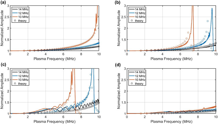
Figure 7. Wave amplitudes in a plasma for different propagation modes. Each color denotes a specific source frequency of the wave, with the solid lines corresponding to FARR simulations and the circles corresponding to the WKB theory. The amplitudes are all normalized to the initial value. (A) O-mode. (B) X-mode. (C) R-mode. (D) L-made.

3.2 Comparison with PHaRLAP

As part of the validation of FARR, we compare simulations to the numerical ray tracing code PHaRLAP (Cervera and Harris, 2014) under a background ionosphere provided by IRI 2020 (Bilitza et al., 2022). Given the smoothly varying plasma density with only large scale gradients, the geometric optics approximation is applicable, and both FARR and PHaRLAP should provide similar results. The background plasma density from IRI begins at an altitude of approximately 65 km, with an foE = 1.15 MHz and hoE = 108 km. The altitude at which the plasma frequency matches 1 MHz is 96.75 km.

Using PHaRLAP we simulate a 1 MHz ray launched at a 60$°$ elevation angle, and consider the height of reflection, time of flight, angle of arrival, and 1st hop distance. Here we use the 2D numerical ray tracing module in PHaRLAP which neglects the background magnetic field. We provide the same background plasma density to FARR and discretize the grid using 3,000 processors on the Stampede 3 supercomputer at the Texas Advanced Computing Center. The simulation parameters are provided in Table 2. We then launch a 1 MHz sine wave pulse using a 16 element linear array of half-wave dipole antennas, phased to 60$°$ with a 7.16$°$ half power beamwidth (HPBW). The source amplitude is modulated by a Gaussian envelope to provide a 100 kHz bandwidth. For comparison with PHaRLAP, we select the location in the grid with the maximum energy density at each timestep to be the center of the main lobe. Figure 8 compares the path taken by the main lobe in FARR with rays launched in PHaRLAP. With PHaRLAP, rays are launched spanning the HPBW of the antenna array. The location of the wave in FARR is in good agreement with the locations of PHaRLAP rays, with the exception of a small cluster of points at 100 km ground distance that are caused by a sidelobe of the antenna array. Table 3 summarizes the measured parameters, with the 1 hop distance for PHaRLAP being the ray launched at center of the main lobe. The general agreement between the simulations shows that FARR accurately reproduces important characteristics of ray-tracing when the geometric optics limit is valid.

Table 2

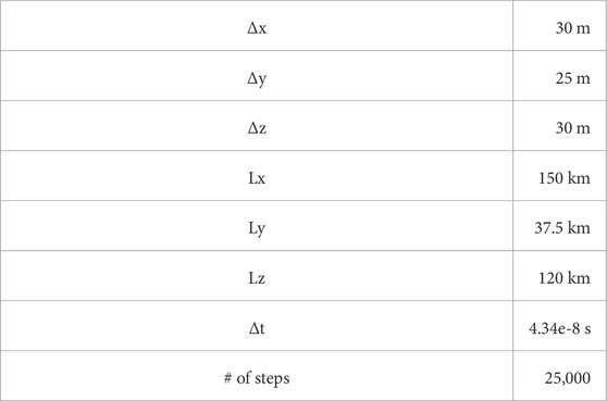
Table 2. FARR simulation parameters for comparison with PHaRLAP.

Figure 8

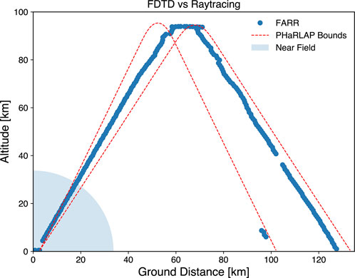
Figure 8. Comparison of 1 MHz ray path in FARR vs. PHaRLAP. Blue dots indicate the location of maximum energy in the main lobe at each timestep in FARR (tracing the ray path). Red dashed lines indicate rays launched in PHaRLAP spanning the HPWB of the array. The small cluster of blue points at 100 km ground distance is due to a sidelobe of the antenna array backscattering from the ground. We also highlight the near field region (within the Fraunhofer distance) where we expect significant discrepancies between raytracing and FDTD.

Table 3

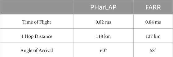
Table 3. Measured parameters from FDTD/raytracing comparison.

4 Discussion

FARR is a full-feature, documented, large scale code for modeling electromagnetic waves in a plasma. Smaller problems with reduced dimensionality can run on desktop computers (e.g., Figure 7), while larger scale simulations (e.g., Figure 8) scale well with high performance computing resources. The code has a variety of boundary conditions and incident source waves to model a wide range of problems. In particular, the TFSF method and antenna array modules allow for realistic, finite bandwidth wave forms to be introduced to a region containing an inhomogeneous plasma. The code automatically selects a routine for updating the current density in the plasma based on the input magnetic field and collision rates. Simulation size can be reduced by utilizing the near-to-far field post-processing routines, eliminating the need to propagate waves through a large region of free space.

By design, FARR can one-way couple to any plasma simulator using a Python pre-processing routine. To do this coupling, approximately 10 lines of Python code from an example routine on the Gitlab repository need to be modified to read in the simulated plasma density from a file. The routine will then interpolate this density onto a regular grid based on the FARR simulation parameters, creating an HDF5 file with a standardized plasma frequency at each time step needed for FARR. This one-way coupling is easy to setup, and the scalability of FARR allows for a wide variety of studies of electromagnetic propagation through a plasma. It should be noted that one current limitation of FARR is that it utilizes a Cartesian grid, and therefore is not well suited for problems involving global propagation of waves.

The validation tests in Section 3 show the potential for FARR to model wave propagation in the ionosphere. The setup for testing O, X, R and L mode propagation is similar to an ionosonde setup. Future studies can expand this setup to simulate ionograms from either a smoothly varying or turbulent ionosphere. By increasing the frequency to the VHF range, this setup can simulate the radar backscatter off of ionospheric irregularities. The comparison of FARR to ray-tracing shows how the code can be used for studying the path HF waves take through the ionosphere. Prior work by Smith et al. (2020b) has shown the viability of the FDTD method for modeling SuperDARN propagation through an irregular ionosphere. By coupling FARR to plasma simulations of ionospheric turbulence, SuperDARN propagation can be further studied without the assumptions of geometric optics.

The goal of developing FARR is to model and quantify the effects of scintillation for trans-ionospheric radio signals. Future studies will couple FARR with the Electrostatic Parallel Particle-in-Cell (EPPIC) simulations of the gradient-drift and Farley-Buneman instabilities (Oppenheim and Dimant, 2004; Oppenheim et al., 2008; Oppenheim and Dimant, 2013; Young et al., 2017; Young et al., 2020). FARR is currently capable of simulating the evolution of trans-ionospheric radio waves at HF or lower VHF frequencies. The intensity, phase, and polarization on the ground is captured by the simulation, and therefore any scintillation index can be reconstructed with post-processing. For higher frequencies such as UHF and L-band, scintillation can be studied but at a significant computational cost, since the grid must resolve the wavelength of the signal.

5 Summary

Here we have presented FARR, an open source, high-performance, finite-difference time-domain (FDTD) code for modeling radio wave propagation in inhomogeneous, magnetized plasmas. FARR is a fully featured FDTD code with a variety of boundary conditions, antenna/array and plane wave sources, and a time-domain near-to-far field transform. By using the FDTD method, FARR is naturally able to model both diffractive and refractive processes, as well as finite-bandwidth sources. A key feature in FARR is the ability to easily one-way couple to external models for ionospheric plasma densities. In this paper, we have validated FARR through comparison with raytracing and standard cold-plasma dispersion relations for O, X, L, and R modes. Future studies with FARR will consider both diffractive and refractive scintillation processes, as well as HF/VHF radar backscatter.

As an open source code, FARR is available for community use via the data availability statement below. Researchers should consult the licensing statement on GitLab for using FARR in publications and research, but may freely use the code for educational purposes.

Data availability statement

The datasets presented in this study can be found in online repositories. The names of the repository/repositories and accession number(s) can be found below: https://doi.org/10.5281/zenodo.14025871.

Author contributions

AG: Writing–original draft, Writing–review and editing. WL: Writing–original draft, Writing–review and editing. MO: Writing–original draft, Writing–review and editing. MY: Writing–original draft, Writing–review and editing.

Funding

The author(s) declare that financial support was received for the research, authorship, and/or publication of this article. AG, WL, MO, and MY were supported by NASA LWS grant 80NSSC21K1322. This work used Stampede 3 at the Texas Advanced Computing Center through allocation EES240116 from the Advanced Cyberinfrastructure Coordination Ecosystem: Services & Support (ACCESS) program, which is supported by U.S. National Science Foundation grants #2138259, #2138286, #2138307, #2137603, and #2138296.

Acknowledgments

The authors acknowledge the Texas Advanced Computing Center (TACC) at The University of Texas at Austin for providing HPC resources that have contributed to the research results reported within this paper (http://www.tacc.utexas.edu).

Conflict of interest

The authors declare that the research was conducted in the absence of any commercial or financial relationships that could be construed as a potential conflict of interest.

Generative AI statement

The author(s) declare that no Generative AI was used in the creation of this manuscript.

Publisher’s note

All claims expressed in this article are solely those of the authors and do not necessarily represent those of their affiliated organizations, or those of the publisher, the editors and the reviewers. Any product that may be evaluated in this article, or claim that may be made by its manufacturer, is not guaranteed or endorsed by the publisher.

References

Bécache, E., Fauqueux, S., and Joly, P. (2003). Stability of perfectly matched layers, group velocities and anisotropic waves. J. Comput. Phys. 188, 399–433. doi:10.1016/s0021-9991(03)00184-0

CrossRef Full Text | Google Scholar

Bellan, P. M. (2006). Fundamentals of plasma physics. Cambridge University Press.

Google Scholar

Bilitza, D., Pezzopane, M., Truhlik, V., Altadill, D., Reinisch, B. W., and Pignalberi, A. (2022). The international reference ionosphere model: a review and description of an ionospheric benchmark. Rev. Geophys. 60, e2022RG000792. doi:10.1029/2022rg000792

CrossRef Full Text | Google Scholar

Cervera, M. A., and Harris, T. J. (2014). Modeling ionospheric disturbance features in quasi-vertically incident ionograms using 3-d magnetoionic ray tracing and atmospheric gravity waves. J. Geophys. Res. Space Phys. 119, 431–440. doi:10.1002/2013JA019247

CrossRef Full Text | Google Scholar

Chevalier, T. W., Inan, U. S., and Bell, T. F. (2008). Terminal impedance and antenna current distribution of a vlf electric dipole in the inner magnetosphere. IEEE Trans. Antennas Propag. 56, 2454–2468. doi:10.1109/TAP.2008.927497

CrossRef Full Text | Google Scholar

Coster, A., and Komjathy, A. (2008). Space weather and the global positioning system. Space Weather. 6. doi:10.1029/2008SW000400

CrossRef Full Text | Google Scholar

Godoy, W. F., Podhorszki, N., Wang, R., Atkins, C., Eisenhauer, G., Gu, J., et al. (2020). ADIOS 2: the adaptable input output system. a framework for high-performance data management. SoftwareX 12, 100561. doi:10.1016/j.softx.2020.100561

CrossRef Full Text | Google Scholar

Guiffaut, C., and Mahdjoubi, K. (2000). “A perfect wideband plane wave injector for fdtd method,” in IEEE antennas and propagation society international symposium. Transmitting waves of progress to the next millennium. 2000 digest (Held in conjunction with: USNC/URSI National Radio Science Meeting), Salt Lake City, Utah: IEEE, 236–239. doi:10.1109/APS.2000.873752

CrossRef Full Text | Google Scholar

Loucks, D., Palo, S., Pilinski, M., Crowley, G., Azeem, I., and Hampton, D. (2017). High-latitude gps phase scintillation from e region electron density gradients during the 20–21 December 2015 geomagnetic storm. J. Geophys. Res. Space Phys. 122, 7473–7490. doi:10.1002/2016JA023839

CrossRef Full Text | Google Scholar

Luebbers, R., Kunz, K., Schneider, M., and Hunsberger, F. (1991). A finite-difference time-domain near zone to far zone transformation (electromagnetic scattering). IEEE Trans. Antennas Propag. 39, 429–433. doi:10.1109/8.81453

CrossRef Full Text | Google Scholar

Merewether, D. E., Fisher, R., and Smith, F. W. (1980). On implementing a numeric huygen’s source scheme in a finite difference program to illuminate scattering bodies. IEEE Trans. Nucl. Sci. 27, 1829–1833. doi:10.1109/TNS.1980.4331114

CrossRef Full Text | Google Scholar

Mrak, S., Semeter, J., Hirsch, M., Starr, G., Hampton, D., Varney, R. H., et al. (2018). Field-aligned GPS scintillation: multisensor data fusion. JGR. Space Phys. 123, 974–992. doi:10.1002/2017ja024557

CrossRef Full Text | Google Scholar

Oppenheim, M., and Dimant, Y. (2004). Ion thermal effects on e-region instabilities: 2d kinetic simulations. J. Atmos. Sol. Terr. Phys. 66, 1655–1668. doi:10.1016/j.jastp.2004.07.007

CrossRef Full Text | Google Scholar

Oppenheim, M. M., Dimant, Y., and Dyrud, L. P. (2008). Large-scale simulations of 2-d fully kinetic farley-buneman turbulence. Ann. Geophys. 26, 543–553. doi:10.5194/angeo-26-543-2008

CrossRef Full Text | Google Scholar

Oppenheim, M. M., and Dimant, Y. S. (2013). Kinetic simulations of 3-d farley-buneman turbulence and anomalous electron heating. JGR. Space Phys. 118, 1306–1318. doi:10.1002/jgra.50196

CrossRef Full Text | Google Scholar

Pokhrel, S., Shankar, V., and Simpson, J. J. (2018). 3-d FDTD modeling of electromagnetic wave propagation in magnetized plasma requiring singular updates to the current density equation. IEEE Trans. Antennas Propag. 66, 4772–4781. doi:10.1109/tap.2018.2847601

CrossRef Full Text | Google Scholar

Roden, J. A., and Gedney, S. D. (2000) Convolution pml (cpml): an efficient fdtd implementation of the cfs–pml for arbitrary media, 27, 334–339. doi:10.1002/1098-2760(20001205)27:5¡334::AID-MOP14¿3.0

PubMed Abstract | CrossRef Full Text | Google Scholar

Samimi, A., and Simpson, J. J. (2015). An efficient 3-d FDTD model of electromagnetic wave propagation in magnetized plasma. IEEE Trans. Antennas Propag. 63, 269–279. doi:10.1109/tap.2014.2366203

CrossRef Full Text | Google Scholar

Sanderson, C., and Curtin, R. (2019). Practical sparse matrices in c++ with hybrid storage and template-based expression optimisation. Math. Comput. Appl. 24, 70. doi:10.3390/mca24030070

CrossRef Full Text | Google Scholar

Smith, D. R., Huang, C. Y., Dao, E., Pokhrel, S., and Simpson, J. J. (2020a). FDTD modeling of high-frequency waves through ionospheric plasma irregularities. JGR Space Phys. 125. doi:10.1029/2019ja027499

CrossRef Full Text | Google Scholar

Smith, D. R., Tan, T., Dao, E., Huang, C., and Simpson, J. J. (2020b). An FDTD investigation of orthogonality and the backscattering of HF waves in the presence of ionospheric irregularities. JGR Space Phys. 125. doi:10.1029/2020ja028201

CrossRef Full Text | Google Scholar

Stix, T. H. (1992). Waves in plasmas. American Institute of Physics.

Google Scholar

Taflove, A., and Hagnes, S. C. (2005). Computational electrodynamics. 3rd edn. Norwood, MA: Artech House Inc.

Google Scholar

Umashankar, K., Taflove, A., and Beker, B. (1987). Calculation and experimental validation of induced currents on coupled wires in an arbitrary shaped cavity. IEEE Trans. Antennas Propag. 35, 1248–1257. doi:10.1109/TAP.1987.1144000

CrossRef Full Text | Google Scholar

Yee, K. (1966). Numerical solution of initial boundary value problems involving maxwell's equations in isotropic media. IEEE Transactions on Antennas and Propagation 14, 302–307. doi:10.1109/tap.1966.1138693

CrossRef Full Text | Google Scholar

Young, M. A., Oppenheim, M. M., and Dimant, Y. S. (2017). Hybrid simulations of coupled farley-buneman/gradient drift instabilities in the equatorial e region ionosphere. JGR. Space Phys. 122, 5768–5781. doi:10.1002/2017ja024161

CrossRef Full Text | Google Scholar

Young, M. A., Oppenheim, M. M., and Dimant, Y. S. (2019). Simulations of secondary farley-buneman instability driven by a kilometer-scale primary wave: anomalous transport and formation of flat-topped electric fields. J. Geophys. Res. Space Phys. 124, 734–748. doi:10.1029/2018JA026072

CrossRef Full Text | Google Scholar

Young, M. A., Oppenheim, M. M., and Dimant, Y. S. (2020). The farley-buneman spectrum in 2-D and 3-D particle-in-cell simulations. JGR. Space Phys. 125. doi:10.1029/2019ja027326

CrossRef Full Text | Google Scholar

Yu, Y., Niu, J., and Simpson, J. J. (2012). A 3-d global earth-ionosphere fdtd model including an anisotropic magnetized plasma ionosphere. IEEE Trans. Antennas Propag. 60, 3246–3256. doi:10.1109/TAP.2012.2196937

CrossRef Full Text | Google Scholar

Yu, Y., and Simpson, J. J. (2010). An e-j collocated 3-d fdtd model of electromagnetic wave propagation in magnetized cold plasma. IEEE Trans. Antennas Propag. 58, 469–478. doi:10.1109/TAP.2009.2037706

CrossRef Full Text | Google Scholar