Measurements of LSTID and LSTAD using TEC and GOCE data

This paper presents measurements gathered with the Gravity Field and Ocean Circulation Explorer (GOCE) satellite, TEC values collected in the American sector, and Poynting Flux (PF) derived using the electric and magnetic fields from the Defense Meteorological Satellite Program (DMSP) satellites aiming to elucidate the mechanisms controlling the initiation of large-scale traveling atmospheric disturbances (LSTAD) and the transit and asymmetry of concurrent large-scale traveling ionospheric disturbances (LSTID). LSTADs and LSTIDs measured during twelve intense magnetic storms that occurred between 2011 and 2013 are thoroughly analyzed. The LSTAD/LSTID appearance and characteristics are correlated against the PF values and the auroral oval’s location, measured by the DMSP satellites. GOCE data and TEC values are used to assess the perturbation of the vertical wind and TEC (∂TEC), inter-hemispheric asymmetry of the appearance of LSTIDs, and the role of the different phases of storms and the structures within interplanetary coronal mass ejections (ICME). Emphasis is devoted to examining LSTADs and LSTIDs during the storms of 5–6 August 2011, 15 July 2012, and 17 March 2013, the supporting material reports on the dynamics of LSTADs and LSTIDs for nine additional storms. During most storms, LSTIDs initiate from both auroral ovals and propagate toward the opposite hemisphere. However, on 5 August 2011 and 15 July 2012, LSTIDs moved only from one hemisphere toward the opposite. Close inspection of the TEC perturbation associated with these events indicates that LSTIDS onsets at opposite hemispheres occur at different times and intensities. This timing delay is produced by the difference in the amount of PF deposited in each hemisphere. It is also indicated that LSTAD’s initiation occurs when the PF is above 1 mW/m² and when the lower latitude edge of the auroral oval moves equatorward at 65°. In addition, LSTIDs are observed during the passage of ICME sheath (in 6 storms), magnetic clouds (11), and Sunward Loops (1), although they occur when the IMF B_z is predominantly directed southward. The observations suggest that the interhemispheric asymmetries in the LSTIDs initiation, extension, and amplitude occur when the ICME sheath passes, containing rapidly varying IMF B_z sign fluctuations. TEC perturbations associated with the LSTID can be up to 4% of the background TEC value, and the LSTAD neutral density variability measured by GOCE can be up to 8%. LSTIDs are observed during all phases of magnetic storms.

Highlights

•TEC and GOCE measurements are analyzed to understand the initiation of LSTADs and LSTIDs during 12 magnetic storms.

•LSTADs are initiated when the Poynting Flux is >1 mW/m² and the auroral oval expands below 65°.

•The equatorward motion of the LSTIDs can be highly asymmetric, coinciding with the interhemispheric asymmetry of the Poynting Flux.

1 Introduction

Atmospheric gravity waves (AGW) propagate through the atmosphere and thermosphere, producing neutral gas disturbances named traveling atmospheric disturbances (TAD). These waves transfer momentum and energy through collisions to the ionized gas, originating from traveling ionospheric disturbances (TID) (Hines, 1960). The ∂U wind associated with AGWs can additionally produce an ion motion along the field lines and an E field through a ∂U × B action that maps to the opposite hemisphere, forming conjugate images of the TID (Jonah et al., 2017). The primary source of short and medium-scale GWs resides in the troposphere due to convective plumes, lightning, and tropical storms (Hocke and Tsuda, 2001; Bishop et al., 2006; Valladares et al., 2017). In addition, tsunamis (Makela et al., 2011), earthquakes (Galvan et al., 2011), winds blowing across a mountain range (Smith et al., 2009), and human-made effects such as explosions and fires (Scott and Major, 2018) create medium and short-scale GWs, respectively. These processes can produce TIDs with different characteristics and spatial and temporal scales at almost any latitude. In contrast, large-scale GWs are primarily initiated in the polar regions due to Joule heating deposited in the auroral E− and F-regions during intense magnetic storms. Large-scale GWs commonly initiate at both auroral ovals and propagate toward the opposite hemisphere (Saito et al., 1998; Shiokawa et al., 2002; Valladares et al., 2009), colliding destructively near the magnetic equator.

This paper presents measurements of large-scale TADs (LSTAD) and LSTIDs made possible by the neutral density values derived from the accelerometer sensor on board the Gravity Field and Ocean Circulation Explorer (GOCE) satellite. These measurements are complemented by concurrent observations of TEC using an extensive network of 2000+ GPS and GNSS receivers that operate in the American sector, providing a comprehensive view of the phenomena. During magnetic storms, considerable particle energy and Poynting Flux (PF) increase the frictional Joule heating at auroral latitudes, launching waves in the ionosphere that propagate equatorward with velocities between 400 and 800 m/s. This article presents the results of an investigation that deals with the role of the PF in initiating LSTADs and LSTIDs. To account for the PF energy input, we use calculations derived from observations performed by the fleet of DMSP satellites. These satellites have an ion drift meter and magnetic field sensors (Knipp et al., 2021) and can measure electromagnetic energy. During steady-state conditions, the PF equals the Joule heating (Thayer and Semeter, 2004) deposited at high latitudes. Consequently, this parameter can be used to investigate their role in the onset times of LSTADs and LSTIDs, their characteristics, and equatorward velocities.

The first studies of LSTIDs were conducted by Ho et al. (1996), Ho et al. (1998) using 150+ globally distributed GPS receivers to demonstrate the simultaneous development of TEC perturbations at both north and south auroral regions. The later expansion of the network of GPS receivers in the American and European sectors brought more complete and spatially extended measurements of LSTIDs (Valladares et al., 2009). Nicolls et al. (2004) employed TEC data from GPS receivers in North America and vertical density profiles from Arecibo to derive a 3-D model of LSTIDs. These authors found that TEC perturbations associated with LSTIDs were about 1 TEC unit and were produced by wind pulses that initiated F-layer vertical motions. Balthazor and Moffett (1997) conducted the first modeling study of LSTIDs using a coupled thermosphere, ionosphere, and plasmasphere model to simulate the transit of LSTADs originating from both auroral ovals. The disturbance propagated toward the geographic equator in the thermosphere and interfered constructively, producing significant density and TEC variations. It is believed that the altitude extension of LSTIDs and their phase at the intersection point may control their propagation into the opposite hemisphere. More recently, Bukowsky et al. (2024) coupled the GITM and SAMI3 models to examine the height and latitudinal propagation of LSTIDs. These authors found that LSTIDs can intrude, propagate into the F-region topside, and reach exospheric altitudes.

Substorms have different dynamics from geomagnetic storms; they occur over a few hours and develop relatively frequently (Akasofu, 1964). During substorms, the incoming energy is released from the magnetotail and injected into the oval region. During these events, Joule heating can increase in the auroral regions. Substorms may also influence the formation and characteristics of LSTADs and LSTIDs. This scientific paper does not address this issue.

This publication introduces LSTADs and LSTIDs for twelve intense magnetic storms that developed during the lifetime of the GOCE satellite to show the variability of the density perturbation amplitude and motions. GOCE was launched into a polar orbit (06:00/18:00 local time) on 17 March 2009 (ESA, 2009). Neutral density and winds were derived from the accelerometer measurements (Bruinsma et al., 2014). The DMSP satellites were also launched into closely polar orbits with DMSP-F15 equatorial passes probing solar local times varying between 16.9 and 15.2 h during the 3 years of this study (2011–2013). DMSP-F16 varied between 18.7 and 17.0 for 3 years, and DMSP-F18 orbit changed between 20.1 and 19.9 local time. This publication also intends to unravel the crucial effects of the different phases of magnetic storms and the characteristics of the Interplanetary Coronal Mass ejections (ICME) in initiating LSTADs and LSTIDs.

The outline of this publication follows. The second section describes the amplitude of the neutral density and wind perturbations due to the LSTADs and the ∂TEC values corresponding to three selected magnetic storms. Section 3 presents the relationship between the LSTIDs’ characteristics and evolution and the different characteristics of the ICMEs for three storms presented in Section 2. Section 4 discusses the general characteristics of all twelve magnetic storms and their relationship with solar wind and magnetospheric quantities. Finally, Section 5 presents the conclusions of this study.

2 Analysis of GOCE, DMSP, and TEC data

Research on LSTIDs and TIDs, particularly their association with TEC perturbations, has significantly advanced in the past decade. This is primarily due to the ability to accurately extract the TEC perturbation linked to density changes over large areas, often caused by tropospheric, thermospheric, or magnetospheric influences. In many cases, the origin of these TEC perturbations can be inferred (Vadas and Crowley, 2010; Valladares et al., 2017). It is understood that a downward electromagnetic PF vector in an E region can intensify the Joule heating (J·E), leading to increased ion and neutral temperatures and the generation of upward and downward neutral motions. This substantial energy deposition, mainly in the auroral oval, is anticipated to create a large-scale wave (LSTAD) system that moves poleward and equatorward.

When the PF vector reaches the high latitude E region, large-scale waves with a scale size ranging between 10° and 20° are formed. As shown below, these waves propagate toward lower latitudes and can last a few hours. Zonal displacement is, in a way, inhibited due to the large longitudinal extension of precipitation PF. Based on the GOCE measurements of the neutral wind, the amplitude of the vertical wind associated with these waves is observed to reach amplitudes as large as ±20 m/s. During the lifetime of the GOCE satellite, thirteen intense geomagnetic storms with SYM-H < −100 nT occurred. However, the storm of 13 October 2012 had no GOCE data recorded. Therefore, all other twelve magnetic storms were thoroughly analyzed, ensuring the validity and reliability of our findings. The results of nine storms can be revised in the Supplementary Material.

The rest of this section reports three storms selected based on the variability of their ∂TEC, the downward PF, and the IMF B_z. These events are 5–6 August 2011, 15 July 2012, and 17 March 2013, corresponding to observations during solstice and equinox seasons. All 12 events were analyzed, spanning the solstice (5) and equinox (7). The significance of the satellite data, particularly the combined observations of ∂(Neutral Density), PF, and particle precipitation by the GOCE and DMSP, both flying in the sun-synchronous orbit, ascending during sunset and descending during sunrise, provides an easy way to identify and distinguish thermosphere conditions and the magnetospheric inputs acting on the dawn and dusk sectors. The ∂TEC data from the American continent covers all local times and will be correctly compared to the satellite data, ensuring a comprehensive and sound data analysis.

In addition, the DMSP satellites provide particle precipitation measurements that allow us to infer the locations of the edges of the auroral oval. Our processing and conclusions are also further favored by including additional ancillary data, such as the three components of the IMF and the solar wind’s density, velocity, temperature, and plasma β (Section 3).

2.1 General description of the storms of 2011–2013

Figure 1 shows the SYM-H values (four top panels) and the height of GOCE (four lower panels) corresponding to the last 4 years of the satellite lifetime (i.e., 2010–2013). Using red, this Figure displays thirteen intense magnetic storms (SYM-H < −100 nT) that developed during these years. The lower panels exhibit the daily variability of the satellite’s height, which changed between 260 and 290 km. It remained at this level until August 2012, when it decreased to an average of 260 km. The altitude was further reduced in May 2013, originating the spacecraft’s final decay and reentry in November 2013.

Figure 1

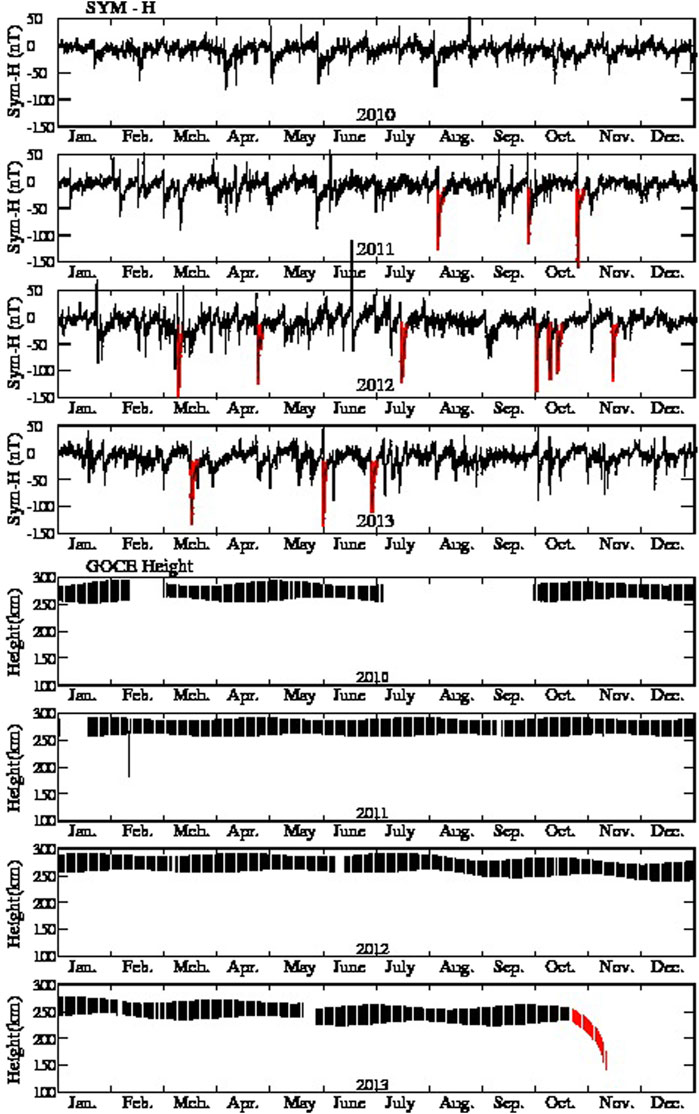
Figure 1. The top four panels display the SYM-H values measured between 2010 and 2013 during the operations of the GOCE satellite. The times of the intense magnetic storms are shaded in red. The lower four panels show the variation in the altitude of the GOCE satellite and the time of reentry in red in November 2013.

Figure 2 displays the neutral density measured by GOCE on 24 May 2011 and between 09:29:50 and 10:00:00. The pass corresponds to the ascending (sunset) phase of the GOCE satellite. At this time, no LSTIDS were present, and no other neutral density fluctuations, such as the equatorial thermal anomaly, were seen at low latitudes (Hocke and Tsuda, 2001; Bishop et al., 2006; Valladares et al., 2017; Makela et al., 2011; Galvan et al., 2011). However, the neutral density presents large variability at polar magnetic latitudes above 80°. To avoid these unwanted high latitude effects, our processing and algorithm extraction of the neutral density perturbation associated with TIDs were restricted to the latitudinal range of −63° and 63°. It is indicated that our analysis aims to identify neutral density changes due to the passage of LSTIDs that start near the auroral oval. We tried different fitting algorithms and found that a 7th-order polynomial curve can reproduce all the essential latitudinal and altitudinal features of the background neutral density variability during non-storm conditions. The upper panel of Figure 2 displays the neutral density in black and the fit in red. The excellent fit produces noise-type differences of less than 3% of the background density. The lower panel of Figure 2 displays in red the difference between the measured neutral density and the 7th-order polynomial fitting. The amplitudes are lower than 0.10 × 10¹¹ Kg or a relative variation of ∼2.5%. As shown below, these differential density profiles develop significant perturbations during intense magnetic storms with amplitudes 4 or 5 times those values.

Figure 2

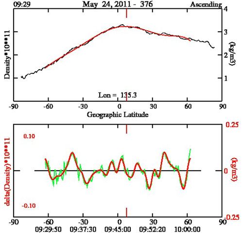
Figure 2. Neutral density data was measured by the GOCE satellite on 24 May 2011. This is a generic plot corresponding to quiet magnetic conditions. The top panel shows this curve’s neutral density and a polynomial fit (red). The lower panel shows the difference between the measured and the fitted curves (green trace) and the filtered trace (in green).

Figure 3 illustrates how we assemble the low-resolution and extended GOCE plots (left panels) that help us identify LSTADs. These observations correspond to three consecutive days, including the magnetic storm’s onset, main, and recovery phases on 5-6 August 2011. This Figure shows consecutive ascending passes, built by removing the background density and vertical wind (see center and right frames) for each pass individually. Both neutral density and the vertical wind values were processed independently using a 7th-order polynomial fit. The center and right frames of Figure 3 show, from top to bottom, the neutral density, the difference between the measured and fitted values, the difference between the processed and fitted vertical wind in green, and the correlation function and the peak of the cross-correlation between the neutral density and vertical wind differences (∂density and ∂wind). The fact that the correlation and cross-correlation are equal implies that the density and wind variability are in phase. The orange arrows point out the relative location of the individual passes and the “low-res” graph on the left. Each pass of GOCE becomes a single vertical line on the left side of Figure 3, with the positive and negative excursions of the differences displayed in red and blue, respectively. The top frame displays the neutral density variability (∂density), and the bottom frame for the vertical wind (∂wind). The usefulness of the “low-res” figure dwells on its ability to provide a rapid and accurate view of the presence of significant ∂density perturbations (e.g., LSTADs). The left frames show high ∂density (top) and ∂wind (bottom) values between 20 UT on 5 August 2011 and 02 UT on 6 August 2011.

Figure 3

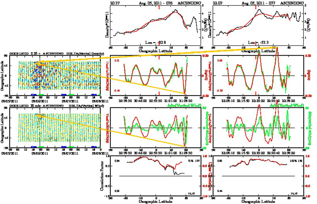
Figure 3. A series of neutral density and vertical wind plots demonstrate how the 3-day low-resolution plots on the left side were constructed. Each vertical line in the left panels corresponds to a density profile taken during the ascending pass, as shown on this figure’s central and right sides. The left panels show the ∂density at the top and ∂(the vertical wind) at the bottom.

2.2 The storm of 5–6 August 2011

Figure 4 shows the SYM-H, the three components of the IMF, and the auroral electrojet (AE) index corresponding to the first intense magnetic storm in 2011. We display 3 days’ worth of data covering the time of the sudden commencement, the main, and part of the recovery phase. The Auroral Electrojet (AE) index is derived from geomagnetic variations in the H component using 10 to 13 magnetic stations located in the northern hemisphere’s auroral zone (Davis and Sugiura, 1966). The AE index represents the overall activity of the electrojets, and the AO index measures the equivalent zonal current averaged over all longitudes. The IMF B_z component is negative (yellow shading) between 18 UT on 5 August 2011 and 04 UT the following day. However, a positive excursion of B_z with sharp boundaries occurred between 22 and 24 UT on 05 August 2011. The commencement and main phases of the storm coincided with this extended period of predominant B_z negative.

Figure 4

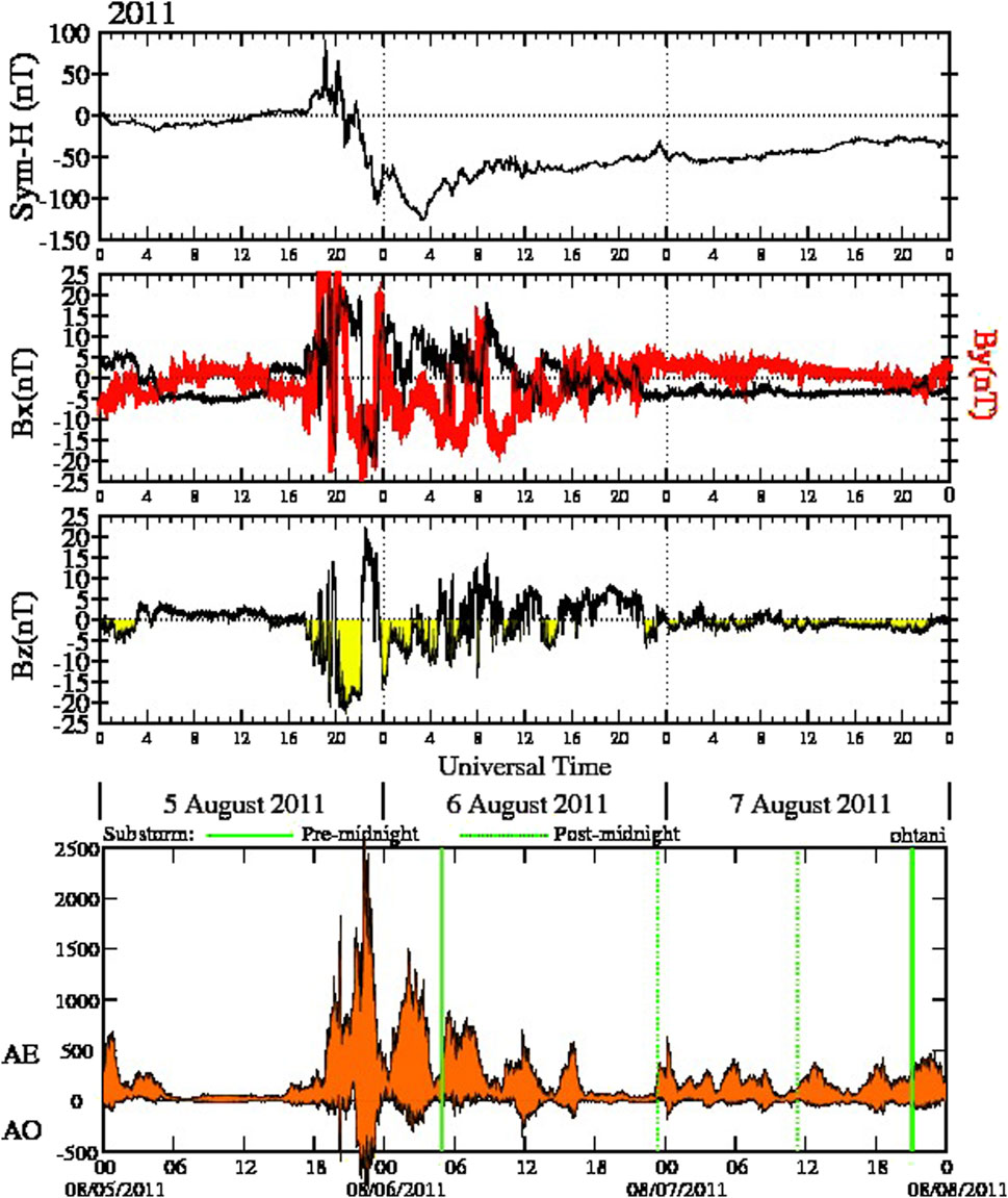
Figure 4. This figure shows solar wind and ionospheric parameters starting 05 August 2011 for three consecutive days. It displays, from top to bottom, the SYM-H values, the IMF B_x and B_y, the B_z parameters, and the AE and AO indices.

Figure 5A illustrates the ground projection of the field lines in the American sector between ±62° magnetic latitude. The ∂TEC values detected within the red region are used to construct the keogram presented in Figure 5B. These field lines cross the magnetic equator between 84° and 76° West longitude. At this longitude, the magnetic field lines are aligned almost parallel to the geographic north-south direction. The ∂TEC values that make the keogram presented here are derived by fitting a running 5th-order polynomial to all the GPS passes and each station individually. The difference between the measured TEC and the fitted curve constitutes the ∂TEC perturbation values associated with the passage of TIDs. Nevertheless, other ionospheric events, such as equatorial plasma bubbles (EPB), can alter the LSTID identification by creating quasi-random features that sometimes obliterate the TID signatures. The resolution of the keogram is 3 min and 0.5° in latitude. The standard deviation of the ∂TEC perturbation is <0.1 TEC units. The transit of the LSTIDs across the continent is seen in the keogram as prominent red and blue slanted lines between 19 UT on 5 August 2011 and 06 UT having amplitudes above 1 TEC unit, indicated by a black arrow near 22 UT. The unique feature of this plot is the consistent southward motion of the LSTIDs that reach −40° geographic latitude and the absence of LSTIDs moving northward. Contrary to these observations, previous measurements and simulations have concluded that LSTIDs initiate almost simultaneously near both auroral ovals and encounter close to the magnetic equator (Valladares et al., 2009; Bukowski et al., 2023). In addition to the LSTIDs, Figure 5B shows several other features, such as small, slanted segments produced by medium and small-scale TIDs and nearly vertical lines seen near 11 UT produced by the morning solar terminator.

Figure 5

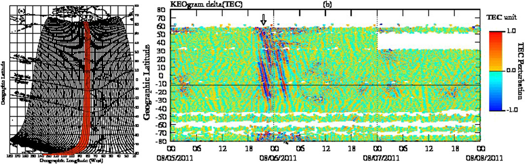
Figure 5. (A) The red band on the left side displays the area used to select ∂TEC values to construct the Keogram displayed on the right side. (B) The dark red and blue diagonal bands represent the LSTIDs measured with the GPS receivers. See the description of this figure for more information on the temporal and latitudinal variability of the keogram.

Figure 6 shows 3 days of “low-res” measurements to demonstrate the intrinsic relationship between the PF, the oval expansion, the development of LSTAD, and the vertical neutral wind perturbation, encompassing the sudden commencement, the main phase and part of the recovery phase of the first storm of 2011. These plots also support our contention that different longitude or MLT sectors have different energy inputs (e.g., PF or particle) and originate LSTADs with distinct characteristics. The eight frames of Figure 6 are labeled descending for sunrise passes (left side panels) and ascending for sunset orbits (right side). From top to bottom, Figures 6A–D show the PF for the northern (between 90° and 50°) and southern hemispheres (between −50° and −90°), the ∂(neutral density), and the ∂(vertical wind). Blue and light blue circles indicate the poleward and equatorward boundaries of the auroral oval, respectively. The dark blue and green dots near the lower horizontal axis indicate times when GOCE crosses the African and South American continents. Panels 6g and h are reproduced from Figure 3 to place the LSTAD differences in the dawn and dusk sectors in context. A significantly enhanced PF is observed right after the beginning of the sudden commencement of the storm (19 UT). The PF energy reaches a value above 0.03 W/m² near 23 UT on 05 August 2011. At the same time, the auroral oval moves equatorward, extending between 55° and 70° in the Northern Hemisphere (NH) and Southern Hemisphere (SH) and for both sunrise and sunset sectors. Concurrently, with the enhanced PF and the expansion of the auroral oval, a significant increase in the ∂(neutral density) variability above the noise level is observed (Figure 6C). An amplitude larger than 20% variations and 20 m/s (Figure 6D) are seen between 22 UT and 06 UT. We believe that the large density and vertical wind perturbations indicate the initiation and transit of LSTADs. The right panels show a different behavior (Figures 6E–H). The ascending passes (near sunset) show an early penetration of the auroral oval to lower latitudes and a higher asymmetry of the northern and southern hemispheres PF. Although the NH reports values above 0.03 W/m², the SH PF contains numbers less than 0.01 and occurs sporadically, delaying the initiation and intensity of LSTADs/LSTIDs in the SH. We believe this lack of PF measurements is due to values smaller than the detectability level of the drift and magnetic field sensors. The earlier oval expansion of the sunset sector, for at least 90 min, is also accompanied by a similar early occurrence of ∂(neutral) perturbations (LSTAD): Figures 6G, H display perturbation extending between 20 UT and 02 UT. Figures 6C, G contain a black line near the bottom of the frame representing the sum of the absolute values of the ∂(neutral density) in percentage. Peak values above 2000 and 1,000 units are observed in the sunrise and sunset sectors, respectively. This line is a good indicator of the presence of LSTADs.

Figure 6

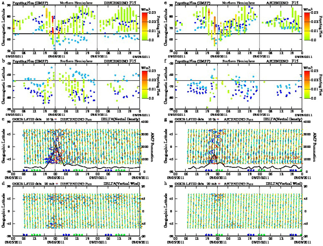
Figure 6. A collage of eight frames showing the PF for the ascending and descending DMSP passes for the northern and southern hemispheres for the same 3 days of Figures 5, 6. (C,D,G,H) Display low-res plots of the neutral density and vertical wind perturbations after analyzing each GOCE pass. The PF intensity is colored from green to red to display values between 0.001 and 0.03 W/m². The blue and light blue dots in panels (A,B,E,F) indicate the boundaries of the auroral oval. The thick line in panels (C,G) points out integrated values of the absolute values of the ∂density.

Figure 7 presents ∂TEC values measured over North, Central, and South America on 5 August 2011. The six frames are separated by 30 min to give a glimpse of the southward motion of the NH ∂TEC and the weak and late initiation of the SH ∂TEC. The encircled numbers designate positive ∂TEC perturbations moving southward in red and northward motions in blue. The ∂TEC increase (red and yellow shadings) seen at 16° geographic latitude (labeled 2) in the image corresponding to 21:00 UT and another detected at −10° (labeled 1) are used to follow the motion of the LSTID. These ∂TEC features are detected 30 min later at 5° and −20°, then at 22 UT move to −5° and −30° latitude, and finally, the frame for 22:30 UT shows the ∂TEC features displaced at −16° and −40° geographic latitude. A series of new LSTIDs is observed to appear later and move southward. Figure 7 indicates that several ∂TEC originating in the NH cross the equatorial line, follow into the opposite hemisphere, and seem to continue up to the southern auroral oval. The image corresponding to 21:30 UT shows the appearance of a weak ∂TEC perturbation at −60° latitude labeled 1 in blue that originates in the SH oval and propagates northward. New ∂TEC moving northward are seen later at 22:30 and 23:00 UT. The nature of this low amplitude LSTID agrees with the weak PF energy deposited in the SH, corroborating a link between PF, Joule heating, and the amplitude of LSTIDs.

Figure 7

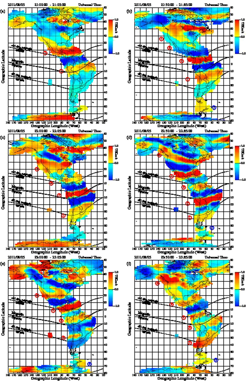
Figure 7. A sequence of 6 ∂TEC maps in the American sector for times extending between 21:00 UT and 23:30 UT. These plots were built by subtracting the TEC daily variability. Positive (negative) ∂TEC perturbations are displayed in red (blue). Note the values peaking at ± 1 TEC units. Red (blue) numbers inside circles indicate the motion of the different ∂TEC layers in the NH (SH). Note very small values of the ∂TEC perturbations near the southern auroral oval. Panel (A) corresponds to 21:00 UT. (B) 21:30 UT. (C) 22:00 UT. (D) 22:30 UT. (E) 23:00 UT. (F) 23:30 UT.

In summary, we observe strong LSTAD and LSTID activity during substantial PF deposition, oval expansion, prominent IMF B_z southward (−20 nT), and concurrent AE index over 2000 nT. The storm LSTADs observed in the sunset sector are detected during the sudden commencement and main phases. The following sub-sections present other cases when LSTAD activity is reported during different seasons, local times, and magnetospheric inputs.

The supporting material contains Supplementary Movie S1, which shows the ∂TEC variability between 17 UT on 5 August 2011 and 02 UT on 6 August 2011. This movie corroborates the steady and spatially uniform motion of the LSTID and provides additional information on the initiation and expansion of ∂TEC perturbations. In the NH, ∂TEC perturbations initiate at 18:03; however, LSTIDs start at 19:18 UT at the SH. The different LSTIDs start times in opposite hemispheres and their unequal velocity and amplitude (LSTAD) make the TIDs encounter at −35° geographic latitude. Although this interaction destroys the SH LSTID, the NH perturbations probably reach the southern auroral oval.

2.3 The storm of 15 July 2012

This storm occurred during the summer solstice (NH), in which the LSTADs presented characteristics similar to those of the 5–6 August 2011 storm. Figure 8 summarizes the ionospheric and magnetospheric parameters that characterize intense storms (e.g., ∂TEC, SYM-H, and IMF). The storm had a lengthy recovery period, with steady IMF B_z near −15 nT lasting 32 h, with a sharp decline and reversal at 14 UT on 16 July 2012. The keogram shows a continuous transit of LSTIDs during the period of B_z southward conditions. However, the LSTIDs show asymmetric motion with a predominant southward direction during the storm’s sudden commencement, a time of B_z rapid sign fluctuations (see arrow near 0 UT on 15 July 2012). This behavior is reminiscent of the LSTIDs observed on the 5 August 2011 storm. However, later that day and during the storm’s recovery phase (after 18 UT and between the second and third arrows), the LSTID motion becomes symmetric, and LSTIDs move simultaneously from both auroral ovals toward the magnetic equator.

Figure 8

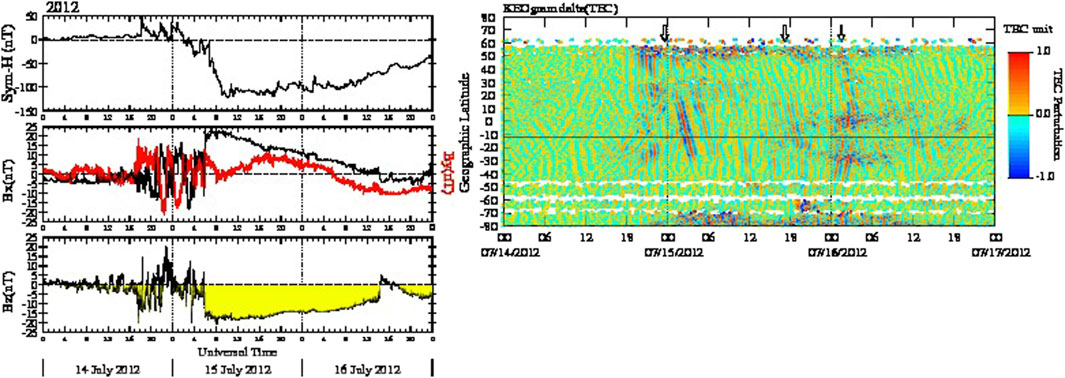
Figure 8. The left side shows the SYM-H and the three components of the IMF for 3 days encompassing the magnetic storm of 15 July 2012. Note the long period of B_x and B_z nearly constant values. The right frame shows the keogram for these 3 days using a format similar to the one in Figure 5.

Figure 9 shows prominent intensifications of the PF and expansions of the auroral oval into latitudes equatorward of 65°. In the NH, the PF penetrates latitudes below 65° at 18 UT on 14 July 2012 during descending (sunrise) and ascending (sunset) passes. This effect is delayed in the SH until 21 UT; here, the PF is also smaller by a factor of 2. The enhanced PF and the oval expansion last 40 h, covering the storm’s commencement, main, and recovery phases. The neutral density and vertical wind perturbations display values more significant than 10% and 20 m/s, respectively. The neutral density perturbations corresponding to sunset (Figures 9G, H) present significant amplitudes exceeding 10% and 20 m/s in the southern hemisphere and not much in the NH. During sunrise (Figures 9C, D), perturbations develop on both NH and SH auroral ovals. Despite the much larger PF in the NH, the LSTADs seem to start simultaneously. The summation traces at the bottom of Figures 9C, H display several periods above the “noise” level.

Figure 9

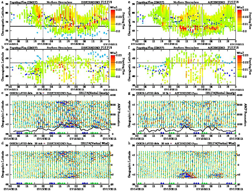
Figure 9. It has the same format as Figure 6 but corresponds to 15 July 2012. Note the long period of intense PF inflow and oval extension up to magnetic latitudes less than 65°. This event coincides with a period of B_z south condition. Large ∂density and ∂(vertical wind) are observed between 06 UT on 15 July 2012 and 06 UT on 16 July 2012. (A,B,E,F) show the Poynting Flux and the boundary of the auroral oval. (C,D,G,H) display low-res plots of the density and vertical wind perturbations.

Figure 10 displays six images of ∂TEC measured between 00:30 and 05:00 UT. This sequence of LSTIDs shows variable and asymmetric behavior in some respects similar to the LSTIDs that developed during the storm of 5 August 2011. Although LSTIDs were triggered from both hemispheres here, the SH LSTIDs compassed much smaller amplitudes and were annihilated near or south of the magnetic equator. The NH ∂TEC continued drifting toward the southern auroral oval, where they faded. The first frame, corresponding to 00:30 UT, shows two positive perturbations labeled with red numbers moving southward and three positive ∂TEC (using blue numbers) drifting northward between South America and Antarctica. The ∂TEC image for 01:00 UT displays the three crests (∂TEC perturbations) using blue numbers displaced further north and crests 1 and 2 (using red numbers) closer to the magnetic equator. The SH LSTID encounters the NH LSTIDs traveling south, destroying the former near the magnetic equator. NH crest 1 (labeled with red numbers) continues moving southward and encounters two more SH crests (labeled 2 and 3 in blue) between 02 and 03 UT, but they are not seen later. The ∂TEC image for 04 UT exhibits the first crest reaching the southern tip of South America across an area devoid of northward-moving LSTIDs. Supplementary Movie S2 shows the LSTIDs’ initiation and departure from both auroral ovals. The organized motion of the LSTIDs starts near 00:30 UT when they initiate a journey to the opposite hemisphere. As indicated above, the movie reaffirms that the motion of the NH LSTIDs to the opposite hemisphere can be asymmetric and destroy the southern LSTIDs at latitudes south of the magnetic equator.

Figure 10

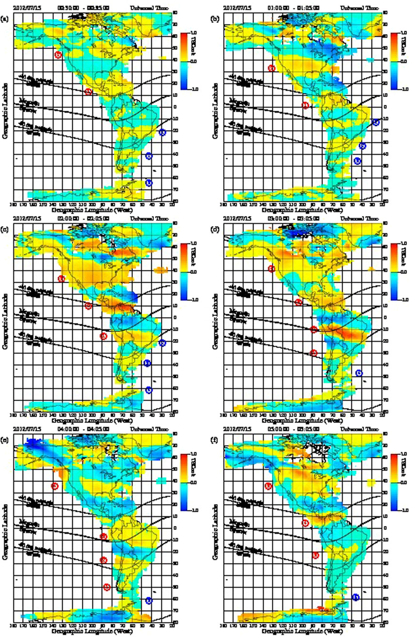
Figure 10. This figure is similar to Figure 7 but corresponds to 15 July 2012. LSTIDs originated in the NH and are seen south of the magnetic equator and transiting at latitudes near the southern auroral oval. See the text for a description of this event. (A) corresponds to 00:30 UT. (B) 01:00 UT. (C) 02:00 UT. (D) 03:00 UT. (E) 04:00 UT. (F) 05:00 UT.

2.4 The storm of 17 March 2013

This event has been called the St. Patrick’s Day Storm of 2013 by Amaechi et al. (2018) and Zhu et al. (2022). Results relevant to our study were conducted by Liu et al. (2018), who reported on the spatial response of the neutral temperature during this storm using SABER and SOFIE measurements. Smith et al. (2009) investigated joule heating asymmetries using the GITM model. Their simulations showed maximum heating in the SH (07:35 UT) and later in the NH (16:40 UT). Other research efforts have compared the St. Patrick Storm of 2013 and 2015 (Xu et al., 2017; Alberti et al., 2017; Dmitriev et al., 2017; Shreedevi et al., 2020). Verkhoglyadova et al. (2016) discussed the storm’s IMF and other solar wind conditions. This section presents LSTADs measured by GOCE and LSTIDs derived from TEC values recorded in the American sector during the St. Patrick’s Day Storm to establish the connection between the magnetospheric PF inputs and the response on the thermosphere and ionosphere. The keogram of Figure 11 displays slanted lines starting from both high-latitude regions and ending near the magnetic equator. This is the signature of LSTIDs propagating toward the opposite hemisphere with nearly equal amplitude and velocity. This Figure demonstrates that during the St. Patrick’s Day Storm of 2013, LSTIDs were observed between 12 and 24 UT (times indicated using 2 arrows). This period is also consistent with both cases presented above in which LSTIDs develop when B_z is directed south, the oval expands, and PF increases to levels higher than 10 mW/m². It is worth noting that this storm generates peak ∂TEC perturbations near 0.5 TEC units. This may be associated with the low value of IMF B_z south and smaller PF than in the other two storms.

Figure 11

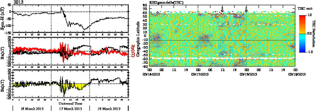
Figure 11. It is the same as Figure 8 but corresponds to the storm on 17 March 2013. This event shows slated lines between 12 and 24 UT on 17 March 2013.

Figure 12 displays the DMSP’s measured PF and the neutral perturbations derived from GOCE’s measurements. Although the NH PF is almost the same in the sunrise and sunset local periods, the afternoon sector SH PF presents an earlier initiation and oval expansion than the NH counterpart (see Figures 12E, F). Higher neutral density and vertical wind perturbations are observed in the morning than in the afternoon local times (Figures 12C, D, G, H). The ∂neutral density is higher than 10%, and vertical wind fluctuations are larger than 20 m/s. Based on this LT asymmetry in the production of LSTADs, it is expected that LSTIDs should be observed mainly around the 12 UT periods when the American continent is in the morning sector. It is indicated that unlike the storm corresponding to 15 July 2012, the St. Patrick’s Day Storm of 2013 shows a B_z southward condition only for 12 h (12 – 24 UT) and values higher than −10 nT.

Figure 12

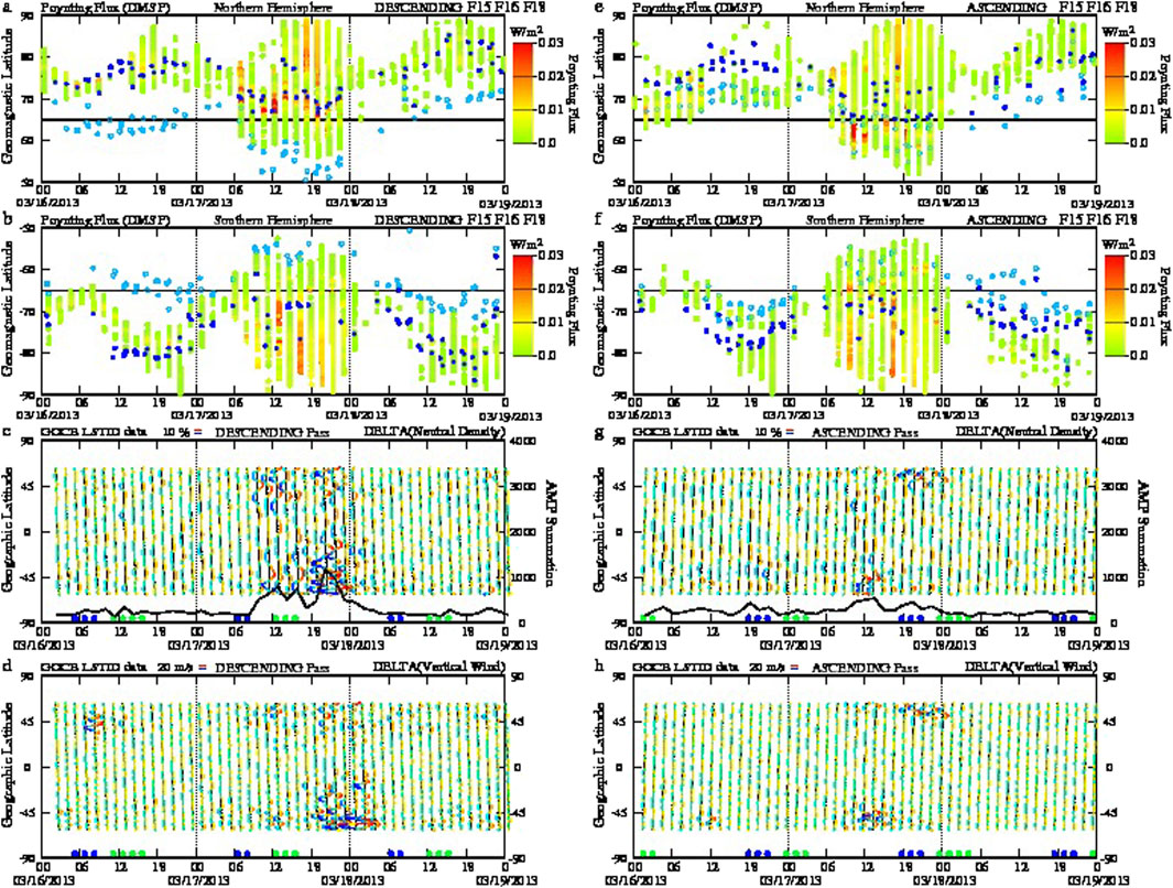
Figure 12. It has the same format as Figures 6, 9 but corresponds to 17 March 2013. A considerably high PF is observed in the northern and southern hemispheres. See the text for a description of LSTIDs getting annihilated near the magnetic equator. (A,B,E,F) show the Poynting Flux and the boundary of the auroral oval. (C,D,G,H) display low-res plots of the density and vertical wind perturbations.

Figure 13 shows a sequence of 6 frames with LSTIDs moving from both high-latitude regions toward the opposite hemisphere and meeting near the magnetic equator. These figures demonstrate that LSTIDs can be generated almost simultaneously, merged, and later annihilated. Frame b corresponding to 17:30 UT exhibits a merging of both positive crests labeled 1 for LSTIDs arising from both hemispheres. This new region labeled 1 in blue keeps moving north, and it is observed at 18 UT (frame c) at 0° geographic latitude, where it vanishes. The SH crest labeled 2 merges with the NH crest labeled 3 after 19 UT, producing a single structure labeled 3 in red in frame f corresponding to 19:30 UT.

Figure 13

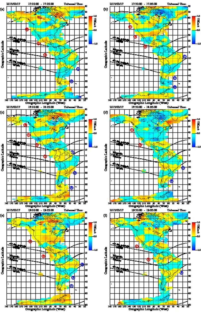
Figure 13. Same format as Figures 7, 10 but for 17 March 2013. Here, the sequence of ∂TEC maps starts at 17:00 UT and extends until 19:30 UT. The amplitude of the LSTIDs is smaller than in both previous storms. (A) corresponds to 17:00 UT. (B) 17:30 UT. (C) 18:00 UT. (D) 18:30 UT. (E) 19:00 UT. (F) 19:30 UT.

Supplementary Movie S3 presents a series of LSTIDs propagating equatorward between 15 and 24 UT. It displays with more detail both sequences of LSTIDs, one from the NH and another from the SH, which encounter near but north of the magnetic equator, where they both annihilate. This behavior of the ∂TEC/LSTIDs is compatible with the keogram of Figure 11, in which the slanted lines (the signature of LSTIDs) between 12 and 24 UT on 17 March 2013 originate from both north and south auroral ovals and meet near the magnetic equator. The motion of the LSTIDs is disorganized near the northern polar cap, likely due to large-scale density structures like storm-enhanced densities. However, at latitudes south of 60°, their variability at constant magnetic longitude and equatorward motion becomes evident.

3 Solar wind dependencies

Intense magnetic storms are attributed to the passage of Interplanetary Coronal Mass Ejections (ICME) that impinge the Earth’s magnetosphere. ICMEs are formed when ejecta material from the Sun interacts with the background non-disturbed solar wind, and a shock is formed in the forefront (Tsurutani and Gonzalez, 1997; Gonzalez et al., 2007). The ICME’s shock is followed by the sheath region that contains elevated solar wind velocity and a highly variable IMF, densities, temperatures, and plasma β. Immediately upstream from the sheath are magnetic clouds (MC), sometimes consisting of sunward or antisunward coronal loops presenting steady IMF, low plasma β, and temperature (Rouillard, 2011; Verkhoglyadova et al., 2016). These different ICME regions can affect the ionosphere and thermosphere differently, inducing distinct responses in the thermosphere-ionosphere system. As stated earlier, this publication deals with forming LSTADs and their indirect visualization in the ionosphere using ∂TEC values measured by GPS receivers. This section aims to find a relationship between the characteristics of the downward PF, the appearance and asymmetry of the LSTADs/LSTIDs, and the passage of ICMEs with different regions. A clear relationship between ICME, PF, and LSTADs will allow us to forecast the initiation of LSTIDs, severity, temporal characteristics, and symmetry/asymmetry.

Figures 14–16 display the three components of the solar wind velocity, the IMF inputs, the density, temperature, and plasma β values (frames from a through j). It also shows the integrated PF along the DMSP trajectory (frame k), a summation of the ∂neutral density detected by GOCE (from the thick line in panels 6c and 6g), and a measure of the LSTIDs amplitude and velocity detected in the American sector using a cross-correlation analysis (frames m, n, o, and p). It is noted that while GOCE and DMSP passes are fixed in a local time frame to near sunset and sunrise hours, ∂TEC measurements occur at all local times. For this reason, a one-to-one comparison between ∂TEC measured in the American sector and satellite observations is made cautiously. These figures also display the different regions of the ICME that have been colored using orange to indicate the sheath region, green to point out the magnetic cloud itself, blue to display a sunward loop connected to the Sun, and yellow to illustrate a high-speed stream (HSS). The arrival time of the ICME shock (https://lweb.cfa.harvard.edu/shocks/wi_data/wi_2012.html), as well as the starting and ending times of the storm magnetic cloud (MC), have been presented (https://wind.nasa.gov/ICME_catalog/ICME_catalog_viewer.php) for solar cycles 23 and 24, and listed by Miteva et al. (2018) and Samwel and Miteva, (2023). These times are used to mark the limits of the different ICME regions. In other cases, we used the solar wind and IMF values described by Verkhoglyadova et al. (2016). These authors indicate that the HSS consists of the solar wind with speeds close to or more than the ICME speed and plasma with variable temperature and β values.

Figure 14

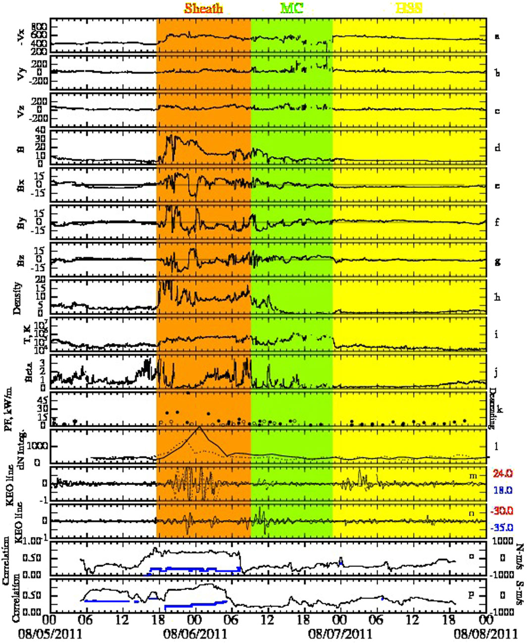
Figure 14. Interplanetary, thermospheric, and ionospheric parameters for days between 05 and 07 August 2011. (A–J) show the three components of the solar wind, the amplitude of the IMF, the three components of IMF B field, the solar wind density, temperature, and the plasma β. (K) displays the PF for the descending passes. The northern hemisphere (SH) flow is shown using full (empty) dots. (L) evinces the integrated absolute value of the ∂density for descending (ascending) passes using a continuous (broken) line. (M,N) show two KEO lines each that have been extracted from the keogram of Figure 5 at two constant geographic latitudes. (O,P) show the peak of the cross-correlation functions and the velocities derived from the offset of the peaks.

Figure 15

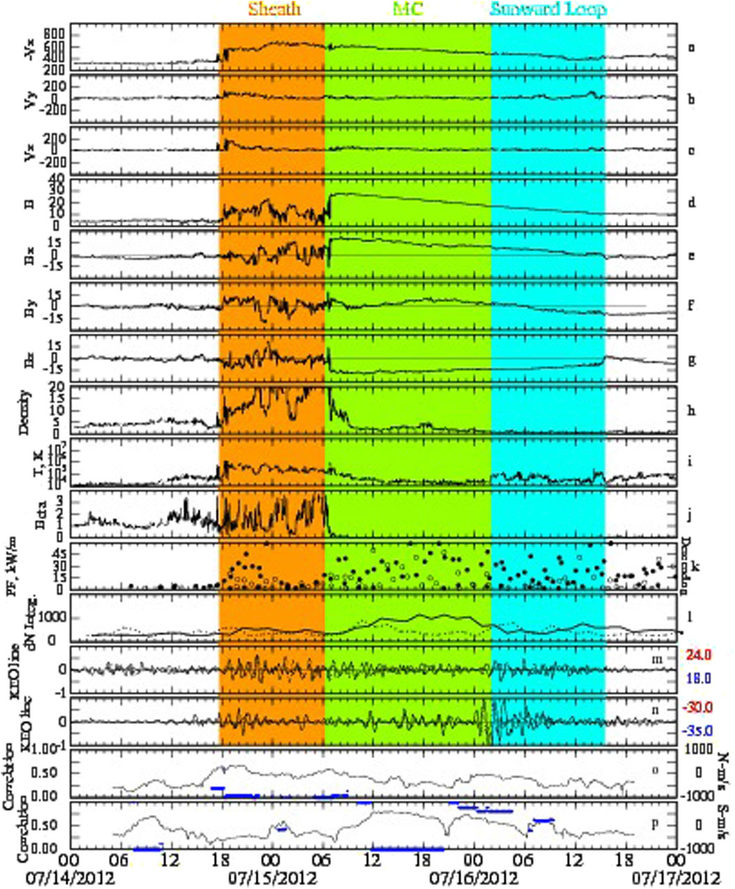
Figure 15. Same as Figure 15 but corresponds to 15 July 2012. (A–L) show the three components of the solar wind, the amplitude of the IMF, the three components of IMF B field, the solar wind density, temperature, the plasma β, the PF, and the integrated absolute value of the ∂density. (M,N) were derived using the keogram of Figure 8. (O,P) show the peak of the cross-correlation functions.

Figure 16

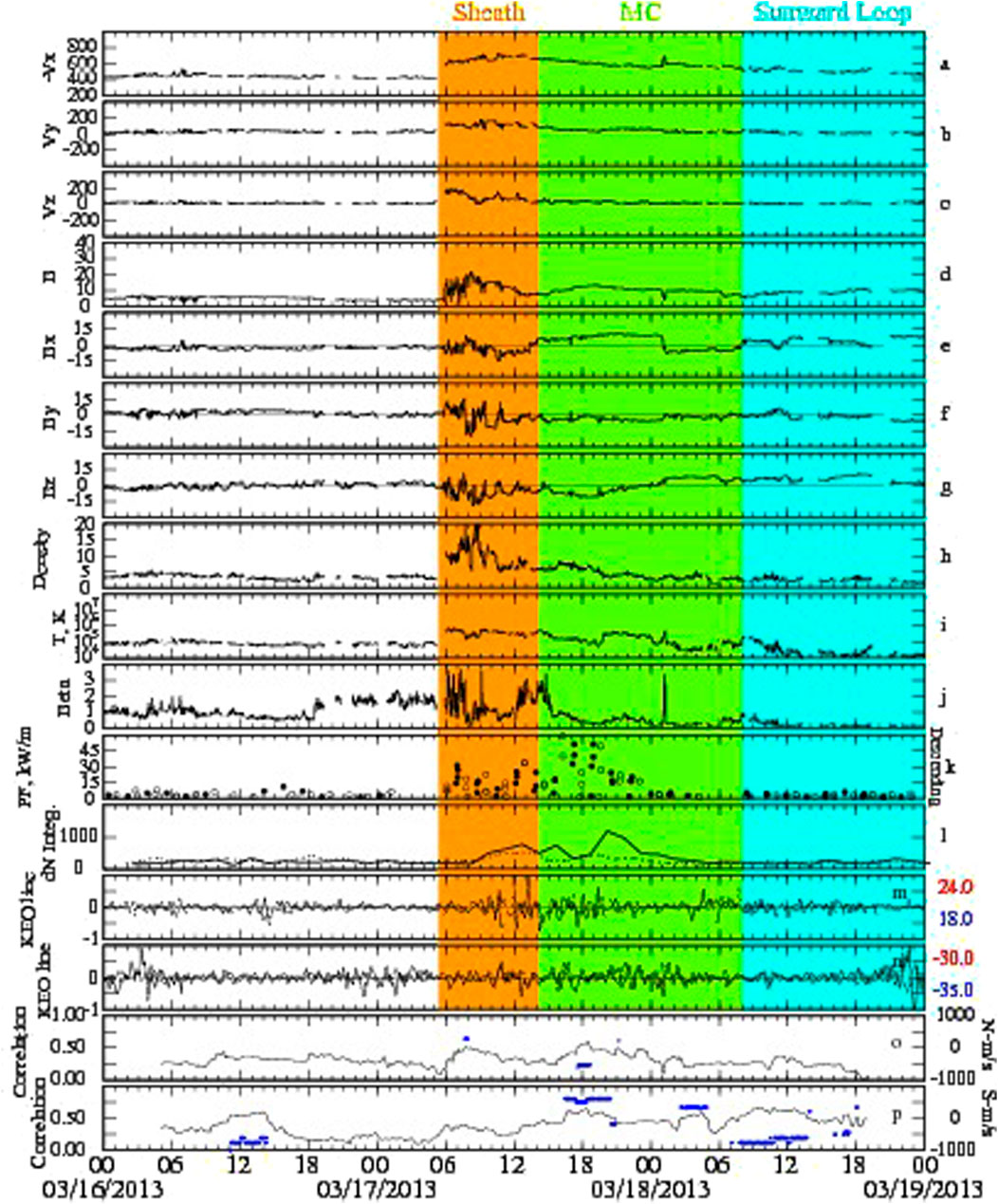
Figure 16. It is the same as Figures 14, 15 but corresponds to 17 March 2013. (A–L) show the three components of the solar wind, the amplitude of the IMF, the three components of IMF B field, the solar wind density, temperature, the plasma β, the PF, and the integrated absolute value of the ∂density. (M,N) were derived using the keogram of Figure 11. (O,P) show the peak of the cross-correlation functions.

3.1 The ICME of 5–6 August 2011

The ICME shock arrived at 17:32 UT on 5 August 2011, followed by an ICME sheath extending until 09:10 UT on 6 August 2011 (Figure 14). The shock was identified as a V_x increase of more than 200 km/s. Simultaneously, the IMF B field grew by 30 nT, the solar wind density, temperature, and plasma β augmented by 15 cm^-3, an order of magnitude, and 15 units, respectively. An MC followed, lasting until 22:40 UT on 06 August 2011, when a sudden increase in the solar wind V_x was seen and decayed on 09 August 2011. This time is beyond the limits of Figure 14.

Figures 14K–P present several parameters derived from direct measurements of the DMSP and GOCE satellites, providing the downward PF and the thermosphere response in the form of LSTADs. In 2011, the ascending orbit of the DMSP-F15 satellite was locked in local time near 16.5 h. Thus, the PF is compared with the ∂TEC measured in the American sector between 20 and 23 UT. The northern hemisphere’s trajectory-integrated PF (full black dots in Figure 14K) reaches quantities above 60 kW/m. This downward PF in the NH is initiated when the IMF B_z becomes less than −5 nT, but later, higher PF values are seen when the IMF B_z is less than −20 nT. In contrast, the PF on the SH (empty circles in Figure 14K) is sporadic and less than 15 kW. The integrated ∂N (Figure 14L), measured by GOCE, increases linearly between the shock and 01 UT on 6 August 2011, when the integrated PF is larger than 60 kW. LSTADs are observed in both the sheath and MC regions; however, no LSTADs are detected during the passage of the high-speed stream (HSS) region. Figures 14M, N show the ∂TEC variations at fixed geographic latitudes. They present a quasi-sinusoidal signature of LSTIDs and are used to calculate the southward velocity of the LSTIDs using a cross-correlation algorithm applied to the ∂TEC fluctuations measured at two pairs of geographic latitudes. One pair at latitudes north of the magnetic equator (24° and 18°) and the other at latitudes south of the magnetic equator (−30° and −35°). The ∂TEC values along these constant latitude lines, called here KEO lines, show an increase in the amplitude of the ∂TEC fluctuations for 24° and 18° (dotted line) geographic latitudes (Figures 14M, N). The peak amplitude and the time delay expressed in m/s provided by the cross-correlation functions are shown in Figures 14O, P. The appearance of LSTIDs in the NH KEO line coincides with the times of large integrated ∂N (Figure 14L) and significant PF in the NH. As stated in section 2.2, the weakened PF < 15 kW/m detected in the SH leads to LSTIDs containing small amplitudes rapidly overrun and annihilated by LSTIDs that move southward from the NH. The cross-correlation algorithm gives downward velocities in both longitude sectors in agreement with the keograms of Figure 5 and the Supplementary Movie S1. In addition, it is significant that the LSTIDs show a decrease in their southward motion (Figure 14P), as seen at later UT times.

3.2 The ICME of 15 July 2012

Figure 15 shows the solar wind, magnetosphere, thermosphere, and ionospheric parameters corresponding to the storm of 15 July 2012 using the same format as Figure 14. This storm also presents well-defined sheath-type ICME characteristics similar to the 5-6 August 2011 storm. The shock arrival is at 17:39 UT on 14 July 2012. The MC starts near 07 UT on 15 July 2012 and ends at 15:30 on 16 July 2012. A part of the MC consists of a sunward loop, where the IMF B_x points toward the Sun. Within the sheath region, the IMF B field contains a B_z south condition during the storm’s first 6 h (18- 24UT). At this time, the downward trajectory-integrated PF rises to 45 kW/m in the NH but only 15 kW in the SH. There is a slight increase in the integrated ∂(neutral density) values, but it is high enough to create significant LSTIDs shown in the KEO line for the NH (Figure 15M). It is indicated that during this period, the keogram of Figure 8 shows barely slanted lines in the NH that reach up to −20° in geographic latitude. No apparent signature of LSTIDs is seen in the SH. Nevertheless, Supplementary Movie S2 displays small ∂TEC perturbations created at 00:30 UT and later at 01:30 UT in the Southern auroral oval.

Between 07 UT on 15 July 2012 and the end of the MC, the integrated PF becomes equal in both hemispheres (see full and empty circles in Figure 15K), increasing to 60 kW/m. In addition, the solar wind density, temperature, and plasma β are low and constant. However, B_x and B_z are large and slowly decrease between 20 and 0 nT. This period coincides with the formation of large (>10%) LSTADs and ∂(neutral wind) (20 m/s) in both descending and ascending orbits and at both the northern and southern hemispheres (Figures 9C, D, G, H). This period also contains several LSTIDs seen, especially near the sunrise (descending passes). The KEOgram of Figure 8 displays equatorial convergent slanted lines that originate at both hemispheres in both north and south auroral ovals. In summary, LSTADs and LSTIDs occur during the early part of the ICME sheath region and later on, all during periods when the IMF B_z is directed southward.

3.3 The ICME of 17 March 2013

Figure 16 displays solar, magnetospheric, and ionospheric parameters similar to the frames shown in Figures 14, 15. The ICME shock occurred at 05:10 UT on St. Patrick’s Day in 2013. At this time, elevated V_x, IMF magnitude, solar wind density, and temperature are identified, defining the start of the sheath region. The MC is observed lasting between 14:10 UT on St. Patrick’s Day and ending on 19 March 2013 (beyond the plot extension). B_z is directed southward between the arrival of the shock and 22 UT on 17 March 2013. During this time, encompassing the sheath and part of the MC, an increase in the integrated ∂N is seen in Figure 16L, together with enhanced PF that maximized at 18 UT on 17 March 2013 (Figure 16K). The amplitude of the KEO lines also rises in Figures 16M, N, together with the cross-correlation factor and the velocity of Figures 16O, P, implying the existence of LSTIDs.

It is indicated that at 08:00 UT on 18 March 2013, a region containing a sunward-directed B_x component, likely connected to the Sun (blue shading), displays no PF above the noise level (Figure 16K), no LSTADs (Figure 16L) and absence of LSTIDs in the KEO lines of Figures 16M, N. This period contains an IMF Bz directed northward that seems to produce unfavorable conditions for the inflow of PF. Contrary to the sunward loop observed on 16 July 2012 (Figure 15), the sunward loop of 18 March 2013 does not reveal any association with LSTADs or LSTIDs.

4 Discussion

We have used several derived physical values measured by the ACE, DMSP, and GOCE satellites to elucidate the solar wind, magnetospheric, and thermospheric conditions that support the formation of LSTIDs. Ground-based observations of ∂TEC data in the American sector have also been analyzed to fully define the asymmetry, amplitude, and timing differences in the appearance of LSTIDs at different hemispheres. Our main conclusion is the dominance of the IMF B_z parameter in dictating the appearance or not of LSTADs and LSTIDs. Our first finding, based on SYM-H values, suggests that these large-scale ∂TEC structures can occur during the sudden commencement, the main phase, or even during the recovery phase of a storm. LSTIDs can happen immediately after the ICME shock, within the sheath region, and during the plasma cloud. Our data also confirms that LSTIDs were observed when the sunward loop passed on 16 July 2012. Figures 14–16 have allowed us to understand the role of PF on the amplitude, asymmetry, and timing of initiating LSTADs. Future constellations of multiple satellites are expected to provide a more robust and precise relationship between solar wind drivers and the ionosphere responses in the form of LSTIDs.

The joint analysis of satellite and TEC data during three intense magnetic storms between 2011 and 2013 has significant implications for the formation, transit, and fate of LSTADs and LSTIDs. Our findings shed new light on the PF measurements during these storms, revealing significant interhemispheric asymmetries and temporal delays that seem to influence the triggering, transit, and sometimes late termination of some LSTADs. The resulting interhemispheric and local time (sunset vs. sunrise) asymmetries are detected in their velocity, amplitude, and the region where the LSTIDs meet. Past experimental and modeling studies have suggested that LSTAD/LSTID should meet near the geographic or magnetic equator, but our results demonstrate that this is not always the case. It is necessary to look carefully at the amplitude and timing of the PF deposited in each hemisphere to determine the meeting location, which can be at the magnetic equator or latitudes as far from the equator as the opposite auroral oval. We observe that when the PF in the NH is three times the value in the SH (Figure 15K), LSTIDs emanating from the southern oval do not pass magnetic latitudes north of −40°.

The PF, thermospheric, and ICME observations for the storms of 05 August 2011 and 15 July 2012 indicated a deep asymmetry in the origin of LSTIDs. However, Supplementary Movies S1, S2 point out the formation of delayed and weak LSTIDs in the SH that are easily overrun by the much stronger NH LSTIDs. LSTIDs in the SH are likely triggered an hour or more later than in the NH. This different behavior between the NH and SH LSTIDs, as well as LSTADs, is based on the asymmetry of the trajectory-integrated PF deposited in both auroral ovals. A common factor during asymmetric behavior is that both cases develop near the start of the storm and during the sheath phase of the ICME. The sheath is commonly characterized by variable solar wind parameters such as the IMF, density, temperature, and plasma β. It is essential to mention that rapid IMF B_z transitions were observed during both storms. These quick changes in the reconnection area may disturb the conjugacy of the PF deposited along the flux tubes. During the passage of magnetic clouds and long periods of constant southward-directed B_z, we observe equal PF in both hemispheres and symmetric LSTIDs that start simultaneously from both north and south auroral ovals that meet near the magnetic equator, where they get annihilated. Systematic analysis of the other 9 intense storms between 2011 and 2013 implies an absence of trajectory-integrated PF and, consequently, no LSTIDs when the IMF B_z is directed north or when the polarity of IMF B_z changes slowly.

It has been demonstrated that the appearance and transit of LSTADs and LSTIDs mainly occur during southward B_z conditions, and strong events develop under steady values less than −15 nT. The PF is larger than 1 mW/m^2, and the auroral oval moves equatorward at 65° (−65° magnetic latitude in the southern hemisphere). The trajectory-integrated PF is at least 5 kW/m. In summary, the key factors leading to LSTAD activity are IMF B_z directed southward and, concurrently, a significant PF. LSTAD generation lasts only as long as the electromagnetic energy is active. It can be as short as a few hours or longer than 24 h (ICME of 15 July 2012).

Several authors have suggested that the PF energy deposited at high latitudes can dissipate as Joule heating in the ionosphere and the thermosphere at altitudes below 200 km (Thayer and Semeter, 2004; Valladares and Carlson, 1991). Lu et al. (1995) used an ionosphere-thermosphere general circulation model to demonstrate that 94% of the PF energy is converted into Joule heating. This heat source then increases the temperature, leading to density and wind flow increases (Mayr and Harris, 1978). An essential product of this change in energy transfer is the production of waves that propagate equatorward with a vertical wind component and propagate equatorward. It is also expected that auroral energy, in the form of electron precipitation, may influence the final amount of heating deposited to form LSTADs.

The low data satellite sampling (100 min between passes) of the LSTADs by GOCE and PF by DMSP satellites prevents us from making a more definite relationship about their temporal chain of events. During the 5-6 August 2011 magnetic storm, we detected a significant asymmetry in the amplitude and the launch time of the LSTADs. We believe the diminishing PF and the limited expansion of the auroral oval in the South produce the late onset time in the southern hemisphere.

Table 1 illustrates and quantifies the patterns of LSTIDs observed during 12 intense magnetic storms (SYM-H < −100 nT). It is indicated that higher PF values produce higher ∂TEC values and asymmetric transit of LSTIDs.

Table 1

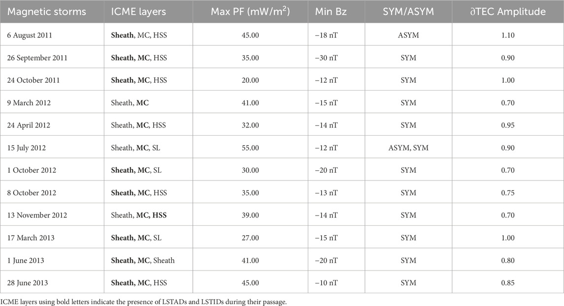
Table 1. LSTID and solar wind characteristics during the storms of 2011–2013.

Our results suggest that most LSTIDs analyzed here move from opposite hemispheres, meet near the magnetic equator, and are typically destroyed. They will likely create a series of smaller-scale structures during their final fate. We have observed that in most cases, LSTADs/LSTIDs encounters occur near the magnetic equator but can develop at other latitudes, as seen on the storms of 5–6 August 2011 and 15 July 2012. This process will undoubtedly increase the ionosphere and thermosphere density “noise” level, which could act as a seed and help initiate EPBs. According to this hypothesis, LSTIDs may have a more significant role. Furthermore, GOCE and TEC data support the role of weak storms in generating LSTADs and LSTIDs (not shown here). These findings underscore the importance of our research and its potential to advance our understanding of LSTADs and LSTIDs significantly.

5 Conclusion

This investigation has led to the following significant findings:

1. A careful analysis of 12 storms (SYM-H < −100 nT) between 2011 and 2013 concluded that LSTID/∂TEC perturbations developed on all 12 storms. Most of the observed LSTID events were seen during the ICME sheath and magnetic cloud. Although a few LSTID events occurred during sunward loops and HSS events. Concurrent LSTADs were detected by the GOCE satellite for each event. Asymmetric or delayed initiation and propagation were observed in two events that happened during the passage of the ICME sheath region. During these cases, asymmetric PF was seen in the northern and southern hemispheres. These two cases (5–6 August 2011 and 15 July 2012) presented rapid polarity reversals of the IMF B_z component. LSTIDs events that developed during the MC or other ICME regions are mainly symmetric with deposited PF equal on both hemispheres.

2. In agreement with previous LSTID observations and simulations, we observed ∂TEC perturbations moving toward the opposite hemisphere. In most events, the LSTIDs encountered were near the geographic or magnetic equator, where they were destroyed and annihilated. However, during the two events mentioned above, the LSTID meeting region was close to the auroral oval in the opposite hemisphere. In these cases, the travel time of the LSTIDs was close to 3 h. The asymmetric LSTIDs behavior was associated with an asymmetric and delayed PF inflow. The amplitude of the LSTIDs observed with a large network of GPS and GNSS receivers was a function of the background TEC that maximizes during the summer solstice months and the equinoxes. Values above 1 TEC unit were found during 7 of the 12 storms.

3. While analyzing these 12 events, we defined two new parameters to help us determine the presence and sources of magnetospheric and thermospheric inputs. One quantity consists of the amount of neutral density perturbation, which is given by the absolute value of ∂(neutral density) integrated between ±63°. The second value is the trajectory-integrated PF measured by the different DMSP satellites. The latter parameter was organized for each hemisphere independently.

4. The GOCE, DMSP, and ∂TEC data presented here show that neutral density and wind perturbations could be as large as 10% and 20 m/s, respectively. The trajectory-integrated PF needs to be as large as a few kW/m to trigger LSTADs. It is suggested that larger PFs generate larger ∂TEC amplitudes. The amplitude of ∂TEC varied between 0.2 and over 1 TEC unit. The minimum threshold of TID detectability is 0,1 TEC unit.

These new results are expected to encourage the development of forecasting capability for the initiation, asymmetry, and intensity of LSTIDs. Solar wind measurements at 1 AU and real-time processing of satellite-measured PF in both hemispheres are suggested as crucial to achieving a forecast capability for LSTADs and LSTIDs. It is also indicated that these new observations would potentially foster a predicting algorithm of LSTID/∂TEC perturbations, inspiring further research and development in this field.

Data availability statement

The datasets presented in this study can be found in online repositories. The names of the repository/repositories and accession number(s) can be found below: https://cdaweb.gsfc.nasa.gov/index.html.

Author contributions

CV: Writing - original draft. Y-JC: Data curation, Investigation, Methodology, Resources, Software, Validation, Writing–review and editing, Writing–original draft. AB: Conceptualization, Data curation, Investigation, Resources, Software, Validation, Writing–original draft, Writing–review and editing. PA: Conceptualization, Data curation, Investigation, Resources, Writing–review and editing, Writing–original draft. PCA: Funding acquisition, Project administration, Resources, Supervision, Validation, Writing–review and editing. SD: Data curation, Investigation, Resources, Writing–review and editing. MH: Data curation, Methodology, Resources, Writing–review and editing.

Funding

The author(s) declare that financial support was received for the research, authorship, and/or publication of this article. The work presented here started when CV was a Research Scientist at the University of Texas at Dallas (UTD) and continued at Boston College (BC). During his tenure at UTD, he was partially supported by NSF Grant AGS-1933056 and NASA Grants 80NSSC20K0195 and 80NSSC20K177. CV was the principal investigator of AFOSR Grant FA9550-21-1-0277, which aimed to expand the low-latitude Ionospheric Sensor Network. At BC, the research was based upon work supported by NASA under award No. 80NSSC23M0193. YC was partially supported by NASA Living with a Star Grant 80NSSC20K1775. PC and SD were supported by NASA grants 80NSSC22K0173 and 80NSSC20K0195. MH partially worked under NASA contracts.

Acknowledgments

The authors also thank NASA/GSFC’s Space Physics Data Facility for making the data available. GOCE data were downloaded from the ESA archive at https://earth.esa.int/eogateway/missions/goce/data, @ ESA (European Space Agency, 2009).

Conflict of interest

The authors declare that the research was conducted in the absence of any commercial or financial relationships that could be construed as a potential conflict of interest.

Generative AI statement

The author(s) declare that no Generative AI was used in the creation of this manuscript.

Publisher’s note

All claims expressed in this article are solely those of the authors and do not necessarily represent those of their affiliated organizations, or those of the publisher, the editors and the reviewers. Any product that may be evaluated in this article, or claim that may be made by its manufacturer, is not guaranteed or endorsed by the publisher.

Supplementary material

The Supplementary Material for this article can be found online at: https://www.frontiersin.org/articles/10.3389/fspas.2025.1517762/full#supplementary-material

References

Akasofu, S.-I. (1964). The development of the auroral substorm. Planet. Space Sci. 12, 273–282. doi:10.1016/0032-0633(64)90151-5

CrossRef Full Text | Google Scholar

Alberti, T., Consolini, G., Lepreti, F., Laurenza, M., Vecchio, A., and Carbone, V. (2017). Timescale separation in the solar wind-magnetosphere coupling during St. Patrick's Day storms in 2013 and 2015. J. Geophys. Res. Space Phys. 122, 4266–4283. doi:10.1002/2016JA023175

CrossRef Full Text | Google Scholar

Amaechi, P. O., Oyeyemi, E. O., and Akala, A. O. (2018). The response of African equatorial/low-latitude ionosphere to 2015 St. Patrick's Day geomagnetic storm. Space weather. 16, 601–618. doi:10.1029/2017SW001751

CrossRef Full Text | Google Scholar

Balthazor, R. L., and Moffett, R. J. (1997). A study of atmospheric gravity waves and travelling ionospheric disturbances at equatorial latitudes. Ann. Geophys. 15, 1048–1056. doi:10.1007/s00585-997-1048-4

CrossRef Full Text | Google Scholar

Bishop, R. L., Aponte, N., Earle, G. D., Sulzer, M., Larsen, M. F., and Peng, G. S. (2006). Arecibo observations of ionospheric perturbations associated with the passage of Tropical Storm Odette. J. Geophys. Res. 111, A11320. doi:10.1029/2006JA011668

CrossRef Full Text | Google Scholar

Bruinsma, S. L., Doornbos, E., and Bowman, B. R. (2014). Validation of GOCE densities and evaluation of thermosphere models. Adv. Space Res 54 (4), 576–585. doi:10.1016/j.asr.2014.04.008

CrossRef Full Text | Google Scholar

Bukowski, A., Ridley, A., Huba, J. D., Valladares, C., and Anderson, P. C. (2024). Investigation of large scale traveling atmospheric/ionospheric disturbances using the coupled Sami3 and GITM models. Geophys. Res. Lett. 51, e2023GL106015. doi:10.1029/2023GL106015

CrossRef Full Text | Google Scholar

Davis, T. N., and Sugiura, M. (1966). Auroral electrojet activity index AE and its universal time variations. J. Geophys. Res. 71 (3), 785–801. doi:10.1029/JZ071i003p00785

CrossRef Full Text | Google Scholar

Dmitriev, A. V., Suvorova, A. V., Klimenko, M. V., Klimenko, V. V., Ratovsky, K. G., Rakhmatulin, R. A., et al. (2017). Predictable and unpredictable ionospheric disturbances during St. Patrick's Day magnetic storms of 2013 and 2015 and on 8–9 March 2008. J. Geophys. Res. Space Phys. 122, 2398–2423. doi:10.1002/2016JA023260

CrossRef Full Text | Google Scholar

European Space Agency, (2009). GOCE thermosphere data collection. Version 1.0. doi:10.5270/esa-l8g67jw

CrossRef Full Text | Google Scholar

Galvan, D. A., Komjathy, A., Hickey, M. P., and Mannucci, A. J. (2011). The 2009 Samoa and 2010 Chile tsunamis as observed in the ionosphere using GPS total electron content. J. Geophys. Res. 116, A06318. doi:10.1029/2010JA016204

CrossRef Full Text | Google Scholar

Gonzalez, W. D., Echer, E., Clua-Gonzalez, A. L., and Tsurutani, B. T. (2007). Interplanetary origin of intense geomagnetic storms (Dst < −100 nT) during solar cycle 23. Geophys. Res. Lett. 34, L06101. doi:10.1029/2006GL028879

CrossRef Full Text | Google Scholar

Hines, C. O. (1960). Can. J. Phys. 38 (11), 1441–1481. doi:10.1139/p60-150

CrossRef Full Text | Google Scholar

Ho, C. M., Mannucci, A. J., Lindqwister, U. J., Pi, X., and Tsurutani, B. T. (1996). Global ionosphere perturbations monitored by the Worldwide GPS Network. Geophys. Res. Lett. 23, 3219–3222. doi:10.1029/96GL02763

CrossRef Full Text | Google Scholar

Ho, C. M., Mannucci, A. J., Sparks, L., Pi, X., Lindqwister, U. J., Wilson, B. D., et al. (1998). Ionospheric total electron content perturbations monitored by the GPS global network during two northern hemisphere winter storms. J. Geophys. Res. 103 (A11), 26409–26420. doi:10.1029/98JA01237

CrossRef Full Text | Google Scholar

Hocke, K., and Tsuda, T. (2001). Gravity waves and ionospheric irregularities over tropical convection zones observed by GPS/MET Radio Occultation. Geophys. Res. Lett. 28, 2815–2818. doi:10.1029/2001GL013076

CrossRef Full Text | Google Scholar

Jonah, O. F., Kherani, E. A., and De Paula, E. R. (2017). Investigations of conjugate MSTIDS over the Brazilian sector during daytime. J. Geophys. Res. Space Phys. 122, 9576–9587. doi:10.1002/2017JA024365

CrossRef Full Text | Google Scholar

Knipp, D., Kilcommons, L., Hairston, M., and Coley, W. R. (2021). Hemispheric asymmetries in Poynting flux derived from DMSP spacecraft. Geophys. Res. Lett. 48, e2021GL094781. doi:10.1029/2021GL094781

CrossRef Full Text | Google Scholar

Liu, X., Yue, J., Wang, W., Xu, J., Zhang, Y., Li, J., et al. (2018). Responses of lower thermospheric temperature to the 2013 St. Patrick's Day geomagnetic storm. Geophys. Res. Lett. 45, 4656–4664. doi:10.1029/2018GL078039

CrossRef Full Text | Google Scholar

Lu, G., Richmond, A. D., Emery, B. A., and Roble, R. G. (1995). Magnetosphere-ionosphere-thermosphere coupling: effect of neutral winds on energy transfer and field-aligned current. J. Geophys. Res. 100 (A10), 19643–19659. doi:10.1029/95JA00766

CrossRef Full Text | Google Scholar

Makela, J. J., Lognonné, P., Hébert, H., Gehrels, T., Rolland, L., Allgeyer, S., et al. (2011). Imaging and modeling the ionospheric airglow response over Hawaii to the tsunami generated by the Tohoku earthquake of 11 March 2011. Geophys. Res. Lett. 38, L00G02. doi:10.1029/2011GL047860

CrossRef Full Text | Google Scholar

Mayr, H. G., and Harris, I. (1978). Some characteristics of electric field momentum coupling with the neutral atmosphere. J. Geophys. Res. 83 (A7), 3327–3336. doi:10.1029/JA083iA07p03327

CrossRef Full Text | Google Scholar

Miteva, R., Samwel, S. W., and Costa-Duarte, M. V. (2018). The Wind/EPACT proton event catalog (1996–2016). Sol. Phys. 293 (2), 27. arXiv:1801.00469. doi:10.1007/s11207-018-1241-5

CrossRef Full Text | Google Scholar

Nicolls, M. J., Kelley, M. C., Coster, A. J., González, S. A., and Makela, J. J. (2004). Imaging the structure of a large-scale TID using ISR and TEC data. Geophys. Res. Lett. 31, L09812. doi:10.1029/2004GL019797

CrossRef Full Text | Google Scholar

Rouillard, A. P. (2011). Relating white light and in situ observations of coronal mass ejections: a review. A Rev. JASTP 73, 1201–1213. doi:10.1016/j.jastp.2010.08.015

CrossRef Full Text | Google Scholar

Saito, A., Fukao, S., and Miyazaki, S. (1998). High resolution mapping of TEC perturbations with the GSI GPS Network over Japan. Geophys. Res. Lett. 25, 3079–3082. doi:10.1029/98GL52361

CrossRef Full Text | Google Scholar

Samwel, S., and Miteva, R. (2023). Correlations between space weather parameters during intense geomagnetic storms: analytical study. Adv. Space Res. 72, 3440–3453. doi:10.1016/j.asr.2023.07.053

CrossRef Full Text | Google Scholar

Scott, C. J., and Major, P. (2018). The ionospheric response over the UK to major bombing raids during World War II. Ann. Geophys. 36, 1243–1254. doi:10.5194/angeo-36-1243-2018

CrossRef Full Text | Google Scholar

Shiokawa, K., Otsuka, Y., Ogawa, T., Balan, N., Igarashi, K., Ridley, A. J., et al. (2002). A large-scale traveling ionospheric disturbance during the magnetic storm of 15 September 1999. J. Geophys. Res. 107 (A6). doi:10.1029/2001JA000245

CrossRef Full Text | Google Scholar

Shreedevi, P. R., Choudhary, R. K., Thampi, S. V., Yadav, S., Pant, T. K., Yu, Y., et al. (2020). Geomagnetic storm-induced plasma density enhancements in the southern polar ionospheric region: a comparative study using St. Patrick's Day storms of 2013 and 2015. Space weather. 18, e2019SW002383. doi:10.1029/2019SW002383

CrossRef Full Text | Google Scholar

Smith, S., Baumgardner, J., and Mendillo, M. (2009). Evidence of mesospheric gravity-waves generated by orographic forcing in the troposphere. Geophys. Res. Lett. 36, L08807. doi:10.1029/2008GL036936

CrossRef Full Text | Google Scholar

Thayer, J. P., and Semeter, J. (2004). The convergence of magnetospheric energy flux in the polar atmosphere. J. Atmos. Solar-Terrestrial Phys. 66 (10), 807–824. doi:10.1016/j.jastp.2004.01.035

CrossRef Full Text | Google Scholar

Tsurutani, B. T., and Gonzalez, W. D. (1997). “The interplanetary causes of magnetic storms: a review,” in Magnetic storms. Editors B. T. Tsurutani, W. D. Gonzalez, Y. Kamide, and J. K. Arballo (Washington, D. C: American Geophysical Union). doi:10.1029/GM098p0077

CrossRef Full Text | Google Scholar

Vadas, S. L., and Crowley, G. (2010). Sources of the traveling ionospheric disturbances observed by the ionospheric TIDDBIT sounder near Wallops Island on 30 October 2007. J. Geophys. Res. 115, A07324. doi:10.1029/2009JA015053

CrossRef Full Text | Google Scholar

Valladares, C. E., and Carlson, H. C. (1991). The electrodynamic, thermal, and energetic character of intense Sun-aligned arcs in the polar cap. J. Geophys. Res. 96 (A2), 1379–1400. doi:10.1029/90JA01765

CrossRef Full Text | Google Scholar

Valladares, C. E., Sheehan, R., and Pacheco, E. E. (2017). “Observations of MSTIDs over south and Central America,” Ionospheric Space weather longitude and hemisphere dependences and lower atmosphere forcing, geophysical monograph. Editors F.-R. Yizengaw, P. H. Doherty, and S. Basu 1st Edn (John Wiley and Sons, Inc), 220.

Google Scholar

Valladares, C. E., Villalobos, J., Hei, M. A., Sheehan, R., Basu, Su., MacKenzie, E., et al. (2009). Simultaneous Observation of traveling ionospheric disturbances in the northern and southern hemispheres. Ann. Geophys 27, 1501–1508. doi:10.5194/angeo-27-1501-2009

CrossRef Full Text | Google Scholar

Verkhoglyadova, O. P., Tsurutani, B. T., Mannucci, A. J., Mlynczak, M. G., Hunt, L. A., Paxton, L. J., et al. (2016). Solar wind driving of ionosphere-thermosphere responses in three storms near St. Patrick's Day in 2012, 2013, and 2015. J. Geophys. Res. Space Phys. 121, 8900–8923. doi:10.1002/2016JA022883

CrossRef Full Text | Google Scholar

Xu, Z., Hartinger, M. D., Clauer, C. R., Peek, T., and Behlke, R. (2017). A comparison of the ground magnetic responses during the 2013 and 2015 St. Patrick's Day geomagnetic storms. J. Geophys. Res. Space Phys. 122, 4023–4036. doi:10.1002/2016JA023338

CrossRef Full Text | Google Scholar

Zhu, Q., Lu, G., Maute, A., Deng, Y., and Anderson, B. (2022). Assessment of using field-aligned currents to drive the Global Ionosphere Thermosphere Model: a case study for the 2013 St Patrick’s Day geomagnetic storm. Space weather. 20, e2022SW003170. doi:10.1029/2022SW003170

CrossRef Full Text | Google Scholar