Fragmentation of young massive clusters in binary components: an application of Griddy Gibbs Sampler

The study of the process of hierarchical fragmentation of molecular clouds within Young Massive Clusters required modeling the Initial Mass Function by considering both binary and single-star components. Components of masses from the Gaia Early Data Release 3 (EDR3) dataset were estimated using the mass–luminosity relationship and the contribution of each mass to the total system was analyzed in the current research. Stochastic models describing the contribution of each component are developed for binary as well as single stars incorporating the escape mass theory of the assumed pair. Binary masses, fitted to suitable bi-variate distributions, were simulated using Griddy Gibbs sampler, a Markov Chain Monte Carlo (MCMC) algorithm. Stellar masses of single stars were simulated using data from suitable uni-variate distribution. The mass spectrum of the binary, as well as single star components, were then considered together to determine the initial mass function. The resulting mass function under opacity limited fragmentation scenario is further investigated at different projected distances from the cluster core to the radius where the signature of mass segregation is found.

1 Introduction

From decades, the Initial Mass Function (IMF) has been a key point of interest to astronomers who study the formation of galaxies as well as the expansion of the universe. As first reported by Salpeter (1955) and Scalo (1998) and later developed by Kroupa et al. (1993), IMF constitutes a power-law of the form $\xi =\frac{dN}{d\log m}\propto m^{\mathrm{\Gamma }}$, $m$ being the masses of a star, $N$ the frequency of the stars in the logarithmic mass range $\log m$ and $\log m+d\log m$, $\mathrm{\Gamma }$ being the slope. The existence of the various mass regimes as parts of piecewise functions of the IMF curve has been put forward by various authors, notably by Kroupa (2002), Chabrier (2003), and Chabrier (2005). The observed mass-regimes may be looked upon as the lower mass-regime (for masses $<1M_{\odot }$) and the higher mass-regime (for the masses $1-10M_{\odot }$) with peak (popularly known as the characteristic mass $(m_c)$) occurring around $0.3-0.5M_{\odot }$. The slope obtained in the various mass regimes is of primary concern to astronomers working with the primordial origin of stellar formation. As reported by Salpeter (1955) the slopes of these mass-regimes are denoted by $\mathrm{\Gamma }\sim -1.35$, for the mass range $(0.4M_{\odot },10M_{\odot })$. Considering the linear mass unit of the form $\frac{dN}{dm}\propto m^{\alpha }$ with $\alpha =1-\mathrm{\Gamma }$, the slopes vary from $2.30\pm 0.30$ for masses $(1M_{\odot },20M_{\odot })$ in the higher mass regimes (Sagar and Kumar 2012), $\mathrm{\Gamma }\sim (0,-0.25)$ for the lower mass-regimes with $m_c$ approximately 0.3 $M_{\odot }$. In their review article, Hannebeller and Gurdic (2024) performed an extensive study regarding the nature of IMF, the different mass regimes, slopes at different piecewise functions, physical features of nebula along with the mass segregation scenario. Various authors including Sagar and Kumar (2012), Sagar and Richtler (1991) and Sanner and Geffert (2001) determined the average slope to be $\mathrm{\Gamma }\sim -1.4\pm 0.3$ and $\mathrm{\Gamma }\sim -1.8\pm 0.6$ for the higher mass regimes for masses greater than 1 $M_{\odot }$. Considering several anomalies in the mass spectrum, studies have been carried out by Chattopadhyay et al. (2011), Chattopadhyay et al. (2016) and Sinha (2018). These authors considered the stellar masses in the form of binary and singular components, thereby studying the contribution of each type of fragment into final form of IMF. They also determined the impact of opacity limited mass segregation in the YMCs.

Stars are usually formed as single, binary, or multiple systems; they are usually viewed through their light curves observed through their orbital planes inclined at a definite angle. In the absence of definite observers of stars, there is considerable debate on whether stars belong to a system. Whether a system is gravitationally bound or not determines the name of its classification into various types of binary or multiple components. Some authors such as Duquennoy and Mayor (1991), Fischer and Marcy (1992), and Kouwenhoven et al. (2007) have conventionally studied the binary fragments and have put forward their findings. Authors like Giovinazzi and Blake (2022), Chulkov and Malkov (2022), and Ducati et al. (2011) have studied orbital binaries, spectroscopic binaries, and visual binaries and their contribution to the IMF by observing their physical features. Riaz et al. (2018) have discussed the formation of protostellar binaries along with their physical properties in the early stages of evolution. Sinha (2018) has studied the contribution of binary and single components by developing a stochastic model. In her finding, she has considered the contribution of binary fragments to be 80% whereas single components as 20%. This ratio, i.e., the percentage contribution of binary and single components has been put forward by different authors in indefinite forms, either by direct observation or by simulation. Resolvable binaries though have an impact on the high-mass regimes of the IMF, whereas unresolved binaries may have a very high impact on the low-mass regime. This point has been raised by Kroupa et al. (2019) in their study. Hence, the distinction of a star whether it belongs to a system or was born as single is very crucial for the IMF to be properly measured.

The formation of stars as multiple systems has been studied and presented by many authors (Duquennoy and Mayor, 1991; Fischer and Marcy, 1992; Kouwenhoven et al., 2007; Malkov and Zinnecker, 2001). In another study, various observational and theoretical studies of stars to be formed as parts of a gravitationally bound system have been presented. Stars that are born as multiple systems or as single star systems (which are not gravitationally bound) have been elaborated by (Offner et al. (2023))? On the other hand, various hypotheses on how stars are born as a binary system have been put forward by Malkov and Zinnecker (2001). In the present work, we retain the claim by Malkov and Zinnecker (2001) that all stars are initially born as a system and we carry our work with the assumption that most of the stars are formed as binary system. We have considered the binary data from the Gaia EDR3 database for the current study. In such a dataset, the mass of a star is not directly observable. Therefore, at this point, the mass of the star needs to be estimated in order to make the final form of IMF acceptable.

The mass of a system can be determined through various directly observable physical parameters. One such way is the use of mass–luminosity relationship using the Russell–Vogt theorem as introduced by Russell et al. (1923) and Hertzsprung (1923). The calculation of masses of the binary system is often quite challenging. Detailed information on mass ratio, orbital period, parallax, luminosity, and average distance of each star from their barycenter are some necessary parameters without which masses cannot be estimated. Chulkov and Malkov (2022) derived a synthetic mass-luminosity relationship for main-sequence stars in the G band and used it to determine masses for the binary system, alongside dynamical masses calculated via Kepler’s third law. While previous studies in the field typically had access to binary masses within their datasets, the current research faced a different scenario where such information was not available. This necessitates the estimation of masses using alternative methods (Chulkov and Malkov, 2022). Notably, the concept of escape mass has been considered only by a few authors and the impact of this on the final form of IMF is the major aspect of this work. The present study adopts the approach of considering the total contribution of both binary and single stars based on escape mass considerations (refer to Section 4 for details). The dataset used in this research was obtained from Gaia EDR3. This dataset offers enhanced positional accuracy, parallax measurements, and proper motion data, thus representing a significant advancement in astrometric precision. Due to its increasing wealth of information and improved astrometry, the Gaia EDR3 dataset is a valuable resource for conducting this comprehensive analysis. We estimated the stellar masses using the relationship as described by Chulkov and Malkov (2022) who extensively described the phenomenon for orbital binaries, resolved binaries, optical pairs as well as unresolved binaries. We have considered pairs having positive parallax.

As put forward by Hennebelle and Grudić (2024), the final form of IMF depends upon various stellar parameters including the mass of a star, gravity and turbulence, match number and density function, protostellar jets as well as dust opacity and molecular hydrogen physics. The impact of these factors on the final form is highlighted in the current study. Our primary focus is on the stochastic fragmentation of Young Massive Clusters (YMCs) through investigation of the contribution of binary and single components to the main population of stars resulting through hierarchical fragmentation of molecular clouds and the final form of IMF observed under opacity limited fragmentation scenario. A stochastic model was developed for the fragmented masses. The binary stars, as a part of the population, were simulated using the Izawa bi-variate gamma distribution through the Griddy Gibbs Sampler method. The single stars were generated from a Pareto distribution, truncated at minimum and maximum masses. We thoroughly investigated the patterns of the bi-variate gamma distribution, and their percentage contribution to the total population of stars and identified an appropriate fitting model. The subsequent sections of this work are organized as follows: Section 2 discusses the dataset; Section 3 presents the estimation of the binary as well as masses of single stars, the form of the bi-variate distribution and uni-variate distributions with their parameter estimation and simulation procedures, and Section 4 provides the results and discussions.

2 Data

The data on binary stars were collected from Gaia Early Data Release 3 (Gaia EDR3) (Chulkov and Malkov, 2022; Brown et al., 2021; Vallenari et al., 2023). It contains information of magnitudes, $a^{″}=$ semi-major axis (in arc sec), $\varpi =$ parallax(in milli arc sec, converted to arc sec), $P=$ orbital period(in years) and $M_e=$ the escape mass $(M_{\odot })$ of 3460 binary stars comprising of visual binaries, spectroscopic binaries, eclipsing binaries and unresolved binaries, but they lacked information regarding the masses of stars within the binary systems. In fact, measurements of the mass ratios or the cumulative masses were not present.

3 Methodology

3.1 Estimation of binary masses

For estimating the binary masses, the mass–luminosity relationship diagram introduced by Hertzsprung (Hertzsprung, 1923) and Russell (Russell et al., 1923) is highly useful in the estimation of mass using luminosities. However, the mass obtained from the above relationship is the cumulative mass of the primary and secondary components of the system. On the other hand, using Kepler's third law, one can estimate the cumulative sum of masses of the binary components using Equation 1:

$M_d=\frac{a^{\prime \prime 3}}{{\varpi }^3{P}^2}(1)$

$M_d$ being the cumulative mass, popularly known as the dynamic mass of the system, being estimated from Equation 1. Parallax uncertainties are very common and quite problematic and are associated with errors when dealt with. Chulkov and Malkov (2022) discussed several methods to deal with such uncertainties. Parallaxes with uncertainties, which make up nearly 14.5% of the total dataset, have not been considered. Only parallaxes with positive values have been included. Parallaxes with zero as well as negative values were not considered in the present research. Moreover, the segregation of optical binaries in a physically bound system and the unresolvable binaries that are no longer gravitationally bound are very important. In order to find this out, is to consider their escape velocity $v$ measured from the relative proper motion $\mathrm{\Delta }\mu$ of components, where $\mathrm{\Delta }\mu =\sqrt{{({\mu }_{\alpha 1}-{\mu }_{\alpha 2})}^2+{({\mu }_{\delta 1}-{\mu }_{\delta 2})}^2}$, ${\mu }_{\alpha }$ and ${\mu }_{\delta }$ denote the proper motion in right ascension and declination, respectively, as discussed by Chulkov and Malkov (2022). The resultant escape velocity, $v$, popularly given by the tangential speed of the components, is denoted as $v\approx 4.74\cdot \frac{\mathrm{\Delta }\mu }{\varpi }$. It provides a lower bound for the relative speed of the components $\sqrt{\frac{2G_{0}M}{r}}$, where $r$ represents the projected distance between the binary components. The minimum mass required for a system to be gravitationally bound, called the escape mass $(M_e)$, can be computed with the help of $v$, using the equation 2,

$M_e=\frac{\rho v^2}{2\varpi G_0}(2)$

where $G_0$ is the gravitational constant. For our case, the escape mass, as provided in the EDR3 dataset, was considered and compared with the computed dynamic mass $(M_d)$. The masses for which $M_d<M_e$ is applicable are considered single stars and the rest are considered as binary stars. The respective percentage contributions, as calculated using the above criterion, of binary and single stars are $77\%$ and $23\%$, respectively. We incorporate this finding in our model construction.

The apparent magnitudes $(g)$ as provided in the dataset with their respective parallax can be used to determine the absolute magnitudes $(G)$, using Pogson’s Law. This law incorporates the concept of interstellar extinction $A_G$ corrected to MLR uncertainty errors. In our data, the apparent magnitudes for both components are available. In the present study, data from the brighter components are used for the above calculation. The interstellar extinction component $A_G$ is simulated using $A_G<0.25$ mag, in support of the findings by Chulkov and Malkov (2022). The MLR uncertainties are simulated with a mean of 0 and a variance of 0.4. The absolute magnitude is thus determined using Equation 2.

$G=g+5+5{\log }_{10}\left(\varpi \right)-A_G+{\sigma }_{\text{MLR}}.(3)$

We use the above-obtained values of absolute magnitudes (G) given in Equation (3) to calculate the mass of the brighter component using the approximation formula, as proposed by Chulkov and Malkov (2022),

$\begin{array}{cc}\hfill \log m=& 0.497-0.151G+0.0106G^2+2.48\times 10^{-4}{G}^3-8.55\times 10^{-5}{G}^4\hfill \\ \hfill & -4.13\times 10^{-7}{G}^5+1.93\times 10^{-7}{G}^6\hfill \end{array}.(4)$

The anti-log of the mass, say $m_1$, as obtained from the above equation (Equation 4), serves as the mass of the primary component. To obtain the mass of the secondary component, say $m_2$, $m_1$ is deducted from the previously obtained $M_d$. The pair of the masses $(m_1,m_2)$ is used to find the mass distribution of the binary components as explained in the next section.

3.2 Fitting of binary masses

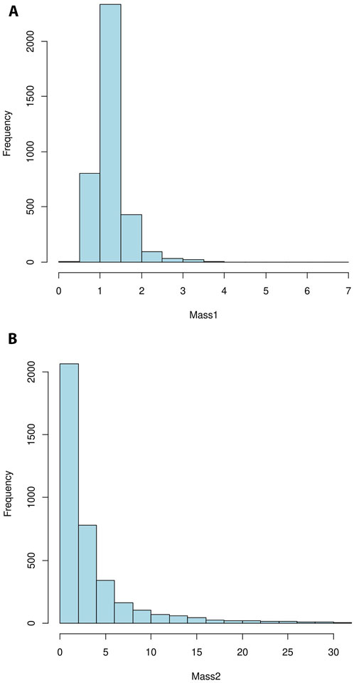
First, we plot the data of the binary masses to study the underlying distribution of masses, as displayed in Figures 1A, B. It can be observed that the binary masses are positively skewed; therefore, a bi-variate gamma distribution suitable for our data is proposed. To model this distribution, we fit a form of bi-variate gamma distribution, namely, the Izawa bi-variate gamma distribution (Izawa, 1965) to our data. The Izawa bi-variate gamma distribution is formulated using the uni-variate gamma marginals and permits distinct scale parameters while maintaining identical shape parameters. The joint PDF of the Izawa bi-variate gamma distribution is given as shown in Equation 5:

$\begin{array}{cc}\hfill f\left(x_1,x_2\right)& =\frac{1}{\mathrm{\Gamma }\left(\nu \right){\left({\beta }_1{\beta }_2\right)}^{\left(\nu +1\right)/2}\left(1-\rho \right){\rho }^{\left(\nu -1\right)/2}}\hfill \\ \hfill & \times {\left(x_1\times x_2\right)}^{\left(\nu -1\right)/2}\exp \left[-\frac{1}{1-\rho }\left(\frac{x_1}{{\beta }_1}+\frac{x_2}{{\beta }_2}\right)\right]\hfill \\ \hfill & \times I_{\nu -1}\left(\frac{2\sqrt{\rho }}{\sqrt{{\beta }_1{\beta }_2}\left(1-\rho \right)}\times \sqrt{x_1{x}_2}\right)\hfill \end{array}(5)$

where $\rho$ is the Pearson’s product–moment correlation coefficient; $\nu$ is the shape parameter; ${\beta }_1,{\beta }_2$ are the scale parameters corresponding to the primary and secondary components of the binary masses, respectively. $I_s$(.) is the modified Bessel function of the first kind (Olver and Lozier, 2010), given by $I_s(h)={\sum }_{m=0}^{\infty }\frac{{(z/2)}^{\nu +2m}}{m!\mathrm{\Gamma }(\nu +m+1)}$. We estimated the four unknown parameters $\nu$, ${\beta }_1,{\beta }_2$ and $\rho$ of the distribution, using the method of moment as suggested by Yue et al. (2001).

Figure 1

Figure 1. (A) Histogram of mass of the primary components in the observed binary system. (B) Histogram of mass of the secondary components in the observed binary system.

The method of moments involves equating the population moments, expressed as a function of the parameters of interest, to their corresponding sample moments and solving for the parameters (Bobee and Ashkar, 1991; Stedinger, 1993). The solutions are estimates of those parameters.

As $\rho$ denotes the Pearson’s product–moment correlation coefficient, it signifies the correlation coefficient estimated from the sample data. It is calculated as shown in equation (6):

$\rho =\frac{E\left[\left(X_1-{\mu }_{X_1}\right)\left(X_2-{\mu }_{X_2}\right)\right]}{{\sigma }_{X_1}{\sigma }_{X_2}}(6)$

Here, (${\mu }_{X_1}$, ${\sigma }_{X_1}$) and (${\mu }_{X_2}$, ${\sigma }_{X_2}$) represent the population mean and standard deviation of $X_1$ and $X_2$, respectively, where $X_1$ and $X_2$ represent mass of the primary component $(m_1)$ and mass of the secondary component $(m_2)$ of the binary system. These components (${\mu }_{X_1}$, ${\mu }_{X_2}$) and (${\sigma }_{X_1}$, ${\sigma }_{X_2}$) are substituted with the sample means ($\overline{X_1}$, $\overline{X_2}$) and sample standard deviations ($s_{X_1}$, $s_{X_2}$). On application of the method of moments, the estimators $\nu =\frac{{\nu }_1+{\nu }_2}{2}$, ${\beta }_1$ and ${\beta }_2$ are calculated. According to the criterion of Izawa bi-variate gamma distribution, we have considered the $\nu$ to be the average of ${\nu }_1$ and ${\nu }_2$, where ${\nu }_i=\frac{{\overline{x_i}}^2}{s_i^2}$, ${\beta }_i=\frac{s_i^2}{\overline{x_i}}$, $\forall i=\mathrm{1,2}$. Finally, the following estimators were derived:

$\begin{array}{c}\hfill {\beta }_1:0.1173508,{\beta }_2:5.991906\hfill \\ \hfill \nu :5.532023,\rho :0.4511818\hfill \end{array}$

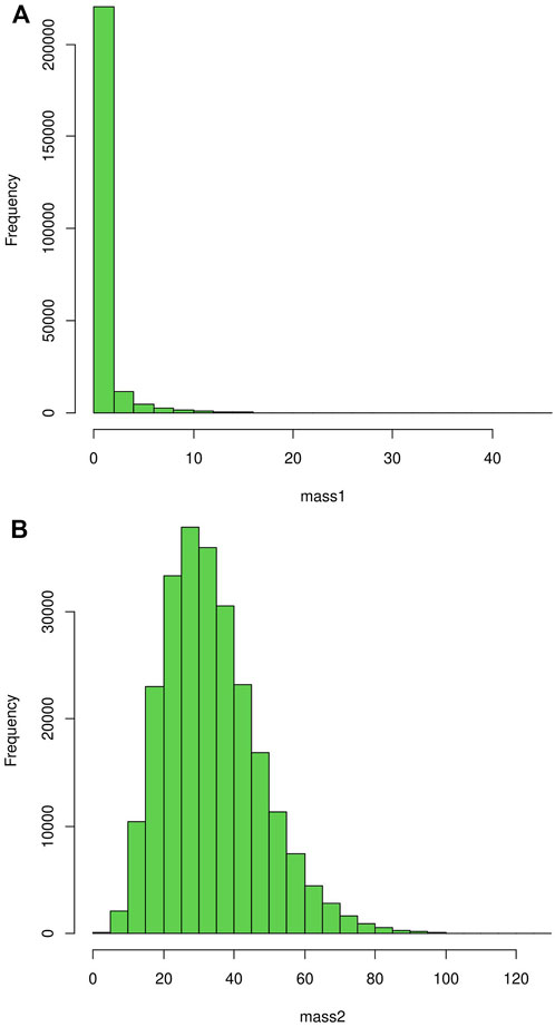
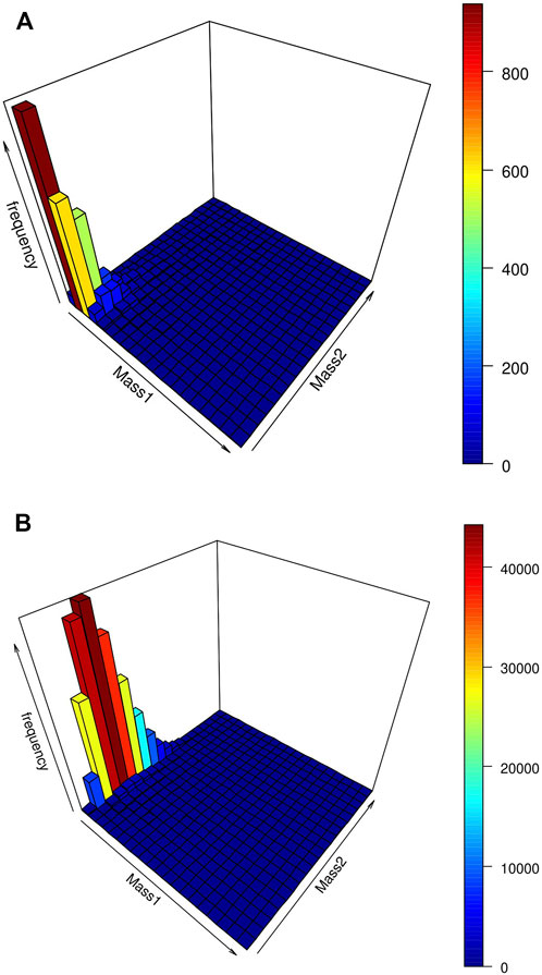
The binary masses are simulated from the Izawa bi-variate gamma distribution with the parameter values as obtained in Section 3.2, by implementing the Griddy Gibbs Sampler as discussed in Section 3.4. The histogram of the primary and secondary components are displayed in Figures 2A, B. The binary components for the observed as well as simulated stellar masses are displayed in Figures 3A, B respectively.

Figure 2

Figure 2. (A) Histogram of mass of the primary components in the simulated binary system. (B) Histogram of mass of the secondary components in the simulated binary system.

Figure 3

Figure 3. (A) Bi-variate histogram of mass of the primary and secondary components in the observed binary system. (B) Bi-variate histogram of mass of the primary and secondary components in the simulated binary system.

The goodness of fit test to see whether the simulated data fit our desired distribution yields a result of ${\chi }^2=68.39$ with a $p$-value = 0.34. Therefore, we accept the null hypothesis which suggests that the observed data follow the Izawa bi-variate gamma distribution. Thereafter, we proceed with the simulation of binary masses from our desired distribution in Section 3.4.

3.3 Fitting of single masses

The single stars are simulated from the Truncated Pareto Distribution as given in an earlier study by Chattopadhyay et al. (2011). The method for generating random samples from the Truncated Power Law distribution, as described by Chattopadhyay et al. (2015) and Chattopadhyay et al. (2016), involves utilizing a segmented power law of the form as given in Equation (7):

${\xi }_{\text{IMF}}\left(m\right)=\frac{dN}{dm}=\left\{\begin{array}{cc}A{m}^{-{\alpha }_1}\hfill & \text{if\hspace{0.17em}}{m}_{\text{min}}<m\le m_c\hfill \\ B{m}^{-{\alpha }_2}\hfill & \text{if\hspace{0.17em}}{m}_c<m\le m_{\text{max}}\hfill \end{array}\right.(7)$

where the parameters $A$ vide Equation 8 and $B$ vide Equation 9 are determined to ensure the following:

$\widehat{A}=B\cdot {\widehat{m}}_c^{{\alpha }_1-{\alpha }_2}(8)$

$\widehat{B}={\left[\frac{m_c^{{\alpha }_1-{\alpha }_2}}{1-{\alpha }_1}\left(m_c^{1-{\alpha }_1}-m_{\text{min}}^{1-{\alpha }_1}\right)+\frac{1}{1-{\alpha }_2}\left(m_{\text{max}}^{1-{\alpha }_2}-m_c^{1-{\alpha }_2}\right)\right]}^{-1}(9)$

The parameters $m_{\mathit{min}}$, $m_{\mathit{max}}$, $m_c$, ${\alpha }_1$, and ${\alpha }_2$ represent minimum mass, maximum mass, critical mass of fragments, and slopes of segmented power laws in a low-mass regime and high mass regimes, respectively. The efficiency factor, $ϵ$, representing the ratio of stellar mass to the total mass of the parent cloud $(m_f)$, as well as the initial values of the parameters, are taken from Sinha (2018). The estimates and results are presented in Section 3.6.

3.4 Fragmentation and mass distribution

The hierarchical fragmentation procedure within molecular clouds in YMCs and in other galaxies, along with the resulting (IMF), has been a topic of significant debate over recent decades. Chattopadhyay et al. (2011) explored the random fragmentation of YMCs through Monte Carlo simulations and treated the number of fragments, the mass of these fragments, and the time intervals between successive fragmentation as the random variables. In their research, masses of binary stars were generated from a bi-variate Gumbel Exponential distribution, and the masses of the single stars from a Truncated Pareto Distribution. They simulated $50\%$ of the total stellar mass of the parent cloud as binary stars, whereas the remaining $50\%$ was attributed to single stars. In Sinha (2018), $80\%$ of the fragment masses were simulated from the bi-variate skew normal distribution for the binary stars and $20\%$ from the Truncated Pareto Distribution for the single stars same as in Chattopadhyay et al. (2011).

In the present work, our primary assumption was that 100% of the total fragments were binary stars. Subsequently, the distinction between binary and single stars was made based on the discussion of escape mass, as explained in the previous section. We retained a choice of $77\%$ of the total stellar mass comprising binary stars, simulated using the Izawa bi-variate gamma distribution, while the remaining $23\%$ comprised single stars, that were simulated using the Truncated Pareto Distribution, as stated earlier.

3.5 Simulation of binary stars

Based on our fitting of the observed masses of binary stars, the simulation of binary masses is conducted using the Griddy Gibbs Sampler method as given by Ritter and Tanner (1992), which is an approximate method of Gibbs Sampling. Gibbs Sampling facilitates generation of random samples from their corresponding conditional density, with a $100\%$ acceptance rate. However, if the analytic form of the conditional distribution is not known or is of some complex form from which direct simulation cannot be done, the method is of limited use. The Griddy Gibbs Sampler acts as an alternative in case of such situations. This method is used to evaluate the conditional density on a grid of points and employ piecewise linear or piece-wise constant functions to estimate the cumulative distribution function (CDF) of the conditional distributions using these grid values so that the resultant random samples generated follow the target distribution, i.e., Izawa bi-variate gamma.

Our conditional distribution, $p(X_i|X_j,j\ne i)$ (say) is nonstandard, and simulating it directly from the conditional density is not possible. The Griddy Gibbs algorithm is applied in the following steps, with a discrete mass of $N$-points:

1. Evaluate $p(X_i|X_j,j\ne i)$ at $X_i=x_1,x_2,\dots ,x_n$, and obtain $w_1,w_2,\dots ,w_n$, by setting $w_j=\frac{p(X_i|X_j,j\ne i)}{{\sum }_{j=1}^{N}p(X_i|X_j,j\ne i)}$.

2. Using $w_j$, approximate the inverse CDF of $p(X_i|X_j,j\ne i)$ by piece wise constant corresponding to a distribution for $x_1,\dots ,x_n$, with probabilities $p(x_i)=\frac{w_i}{{\sum }_{j=1}^N{w}_j}$ or by piece wise linear which corresponds to a piece wise uniform distribution on the interval $[a_i,a_{i+1}]$, $i=1,\dots ,n$, where $x_i$ is in the interval $[a_i,a_{i+1}]$ and the density $f_i$ is given by $\frac{w_i}{{\sum }_{j=1}^n{w}_j}$, where $w_i=w_i(a_{i+1}-a_i)$. Typically, $x_i$ is centered in the interval $[a_i,a_i+1]$.

3. Generate a random number $\sim U_{[\mathrm{0,1}]}$ and invert the approximate CDF to get random samples from $x_1,x_2$.

Here, the mass of the primary component $(m_1)$, specified by $X_1$, and the mass of the secondary component of the binary system $(m_2)$, specified by $X_2$, $i,j=\mathrm{1,2}$, requires the conditional density function to be known up to a certain proportionality constant, of the form as given in equation 10:

$\begin{array}{cc}\hfill f\left(x_1|x_2\right)& =\frac{{\beta }_2^{\nu }}{{\left({\beta }_1{\beta }_2\right)}^{\left(\nu +1\right)/2}\left(1-\rho \right){\rho }^{\left(\nu -1\right)/2}}\hfill \\ \hfill & \times {\left(x_1/x_2\right)}^{\left(\nu -1\right)/2}\exp \left[-\frac{1}{1-\rho }\left(\frac{x_1}{{\beta }_1}+\frac{x_2}{{\beta }_2}\right)\right]\hfill \\ \hfill & \times I_{\nu -1}\left(\frac{2\sqrt{\rho }}{\sqrt{{\beta }_1{\beta }_2}\left(1-\rho \right)}\times \sqrt{x_1{x}_2}\right)\hfill \end{array}(10)$

As previously stated, the conditional density is highly complex, which makes direct simulation from this density unfeasible which validates the application of the Griddy Gibbs Sampler method. We segment the $m_1$ and $m_2$ into several class intervals corresponding to their range of values from which bi-variate relative frequencies for each class interval are determined and used as weights.

3.6 Simulation of single stars

The single masses are simulated from the Truncated Pareto Distribution as mentioned in Chattopadhyay et al. (2011). With the choices of parameters as mentioned in Section 3.3, the random numbers are produced using the inverse transformation method for generating pseudo-random samples from the probability distribution. This method involves generating random samples based on the CDF of the distribution as given in Sinha (2018). By combining the total stellar masses derived from binary fragments and single stars, we establish a segmented power law. This allows us to determine the critical masses and the slopes for various segments.

4 Results and discussion

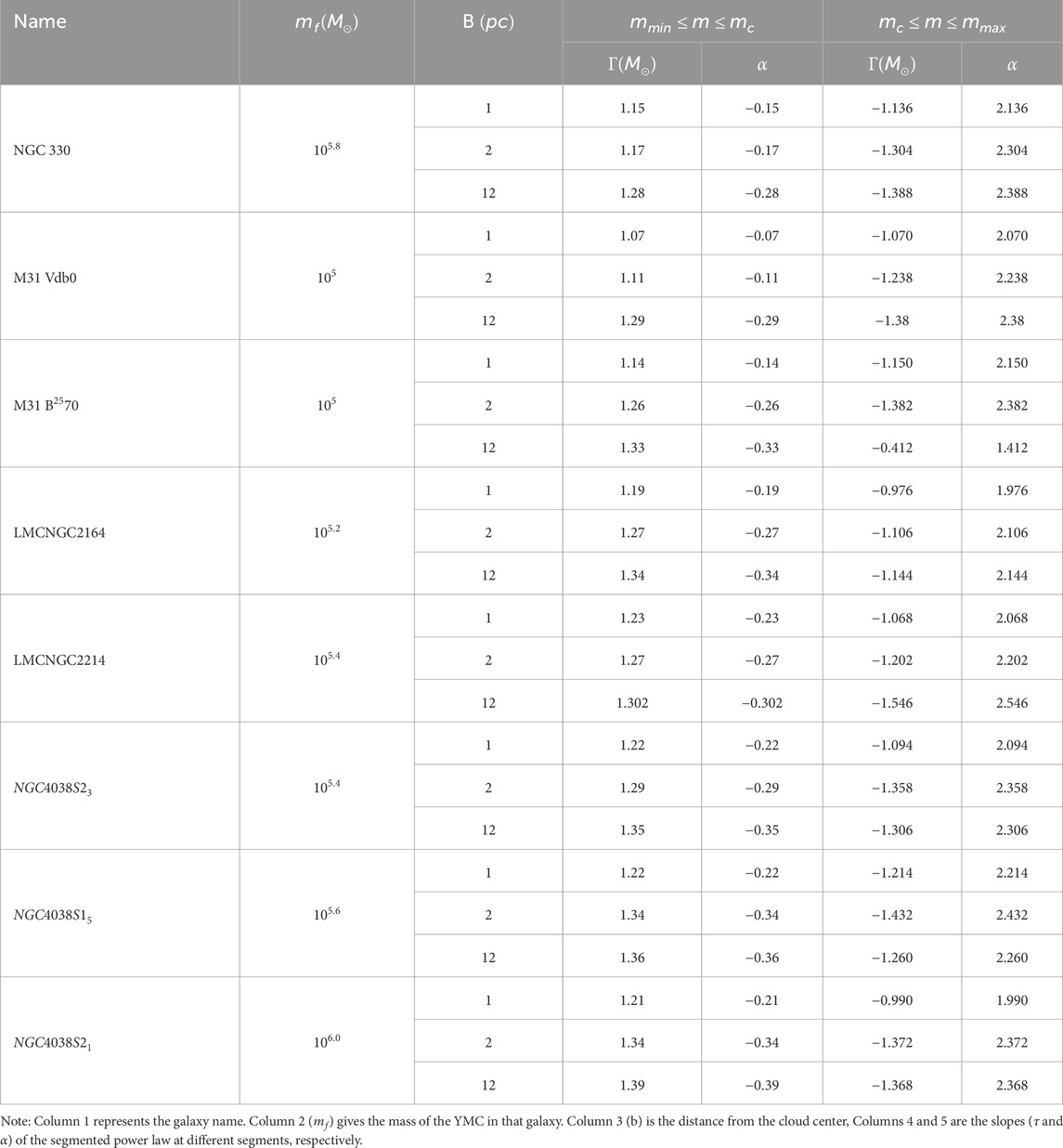
The resultant mass spectrum generated using a combination of masses from binary fragments and single fragments is fitted to segmented power laws in different mass regimes considering the initial parametric values, mass of molecular cloud, efficiency, and other parameters from Sinha (2018). The results are displayed in Table1 along with errors, obtained after repeating each simulation several times. Figure 4 shows the segmented power–law fit for $b=12pc$ for M31Vdb0, with simulated values (given in asterisk). As evident, the mass spectrum shows a steeper slope in all segments compared to earlier studies (Chattopadhyay et al., 2011; Chattopadhyay et al., 2016; Sinha, 2018), mostly in the high mass regimes. Moreover, the signature of mass segregation can be noticed in the form of the slopes for $b=1$ and $b=2$ with a considerable increase in $b=12$, $b$ being the distance from the cloud center. Hence, the findings may be summarized as follows.

$•$ In the previous studies, the masses of the binary stars were observed either from orbital binaries only or from resolvable binaries. Non-resolvable binaries with their masses generated in analog to the escape mass were not considered previously. Resultantly, our previous studies may be assumed to have been based on hypothetical figures of binary masses, whereas more relevant observations (from Gaia EDR3) along with the type of gravitational bound among the binary stars were applied in the present study resulting in the steeper slopes in the high mass regimes.

$•$ Mass segregation appears in the envelope as one moves away from the core, which may be attributed to the results influenced by the rate of primordial binary star formation as well as the creation and destruction of new ones during the star formation epoch Bellazzini et al. (2002).

Table 1

Table 1. Segmented power–law models fitted to the simulated fragments resulting from random fragmentation of young massive clusters (YMCs), accounting for a binary fraction that makes up $77\%$ of the cloud’s total active mass.

Figure 4

Figure 4. Segmented Power–Law fit for M31Vdb0 at $b=12pc$ with the simulated values in asterisk $(\ast )$, $m$ is in $M_{\odot }$.

Hence, the changes observed in the slope of the IMF are due to the inclusion of unresolved binaries, which are gravitationally bound, and primarily recorded as single or high-mass stars or resolvable binaries. Moreover, it is not unknown whether the preliminary drivers determining the star fragmentation procedure are rotation and turbulence Offner et al. (2023), Riaz et al. (2018), the fragmentation procedure of small filaments in dense cores having massive accretion disks leads to multiple or binary system of stars born as protostars. Later, in the evaluation phase, multiplicity or binary declines with time, the binary protostars generally evolving as single stars for losing their gravitationally bound pair. Keeping in view the opacity-limited fragmentation scenario and mass segregation due to cooling from the core of the fragmentation mechanism to the radius, combined with the rotational speed and turbulence of the molecular gas, the presence of smaller stars in multiple systems toward the outer part of the disk of fragmentation is observable, which again leads to the formation of planets and planetary system associated with each star(s) as previously reported by Hannebeller and Gurdic (2024).

To summarize, the study sheds some light into the open questions of star formation and evolution scenarios, when a small number of observable quantities are available at hand.

Data availability statement

Publicly available datasets were analyzed in this study. This dataset can be found here: https://github.com/chulkovd/ORB6.

Author contributions

AS: conceptualization, methodology, project administration, supervision, validation, writing–original draft, and writing–review and editing. AD: data curation, formal analysis, funding acquisition, investigation, resources, software, visualization, and writing–original draft.

Funding

The author(s) declare that no financial support was received for the research, authorship, and/or publication of this article.

Conflict of interest

The authors declare that the research was conducted in the absence of any commercial or financial relationships that could be construed as a potential conflict of interest.

Publisher’s note

All claims expressed in this article are solely those of the authors and do not necessarily represent those of their affiliated organizations, or those of the publisher, the editors and the reviewers. Any product that may be evaluated in this article, or claim that may be made by its manufacturer, is not guaranteed or endorsed by the publisher.

References

Bellazzini, M., Fusi Pecci, F., Messineo, M., Monaco, L., and Rood, R. T. (2002). Deep hubble space telescope wfpc2 photometry of ngc 288. i. binary systems and blue stragglers. Astronomical J. 123, 1509–1525. doi:10.1086/340082

CrossRef Full Text | Google Scholar

Bobee, B., and Ashkar, F. (1991). The gamma family and derived distributions applied inhydrology. Water Resources Publications

Google Scholar

Brown, A. G., Vallenari, A., Prusti, T., De Bruijne, J., Babusiaux, C., Biermann, M., et al. (2021). Gaia early data release 3-summary of the contents and survey properties. Astronomy and Astrophysics 649, A1. doi:10.1051/0004-6361/202039657

CrossRef Full Text | Google Scholar

Chabrier, G. (2003). Galactic stellar and substellar initial mass function. Publ. Astron Soc. Pac. 115, 763–795. doi:10.48550/arXiv.astro-ph/0304382

CrossRef Full Text | Google Scholar

Chabrier, G. (2005). The initial mass function: from salpeter 1955 to 2005. Initial Mass Funct. 50 Years Later 327, 41–52. doi:10.1007/978-1-4020-3407-7_5

CrossRef Full Text | Google Scholar

Chattopadhyay, T., Chattopadhyay, A. K., and Sinha, A. (2011). Modeling of the initial mass function using the metropolis–hastings algorithm. Astrophysical J. 736, 152. doi:10.1088/0004-637x/736/2/152

CrossRef Full Text | Google Scholar

Chattopadhyay, T., De, T., Warlu, B., and Chattopadhyay, A. K. (2015). Cosmic history of the integrated galactic stellar initial mass function: a simulation study. Astrophysical J. 808, 24. doi:10.1088/0004-637x/808/1/24

CrossRef Full Text | Google Scholar

Chattopadhyay, T., Sinha, A., and Chattopadhyay, A. K. (2016). Influence of binary fraction on the fragmentation of young massive clusters—a Monte Carlo simulation. Astrophysics Space Sci. 361, 120–214. doi:10.1007/s10509-016-2705-4

CrossRef Full Text | Google Scholar

Chulkov, D., and Malkov, O. (2022). Visual binary stars with known orbits in gaia edr3. Mon. Notices R. Astronomical Soc. 517, 2925–2941. doi:10.1093/mnras/stac2827

CrossRef Full Text | Google Scholar

Ducati, J. R., Penteado, E. M., and Turcati, R. (2011). The mass ratio and initial mass functions in spectroscopic binaries. Astronomy and Astrophysics 525, A26. doi:10.1051/0004-6361/200913895

CrossRef Full Text | Google Scholar

Duquennoy, A., and Mayor, M. (1991). Multiplicity among solar-type stars in the solar neighbourhood. ii-distribution of the orbital elements in an unbiased sample. Astronomy Astrophysics 248 (2), 485–524.

Google Scholar

Fischer, D. A., and Marcy, G. W. (1992). Multiplicity among m dwarfs. Astrophysical J. Part 396 (1), 178–194. doi:10.1086/171708

CrossRef Full Text | Google Scholar

Giovinazzi, M. R., and Blake, C. H. (2022). A mass–magnitude relation for low-mass stars based on dynamical measurements of thousands of binary star systems. Astronomical J. 164, 164. doi:10.3847/1538-3881/ac8cf7

CrossRef Full Text | Google Scholar

Hannebeller, P., and Gurdic, M. (2024). The physical origin of the stellar initial mass function. Annu. Rev. Astronomy Astrophysics 1, 1–53. doi:10.48550/arXiv.2404.07301

CrossRef Full Text | Google Scholar

Hennebelle, P. G. M., and Grudić, M. (2024). The physical origin of the stellar initial mass function. Annu. Rev. Astronomy Astrophysics 62, 63–111. doi:10.1146/annurev-astro-052622-031748

CrossRef Full Text | Google Scholar

Hertzsprung, E. (1923). On the relation between mass and absolute brightness of components of double stars. Bull. Astronomical Institutes Neth. 2, 15–22.

Google Scholar

Izawa, T. (1965). Two or multi-dimensional gamma-type distribution and its application to rainfall data. Pap. Meteorology Geophys. 15, 167–200. doi:10.2467/mripapers1950.15.3-4_167

CrossRef Full Text | Google Scholar

Kouwenhoven, M., Brown, A., Zwart, S. P., and Kaper, L. (2007). The primordial binary population. ii.-recovering the binary population for intermediate mass stars in scorpius ob2. Astronomy and Astrophysics 474, 77–104. doi:10.1051/0004-6361:20077719

CrossRef Full Text | Google Scholar

Kroupa, P. (2002). The initial mass function of stars: evidence for uniformity in variable systems. Science 295, 82–91. doi:10.1126/science.1067524

PubMed Abstract | CrossRef Full Text | Google Scholar

Kroupa, P., Jerabkova, T., Giacomo, B., and Henri, M. (2019). The impact of binaries on the stellar initial mass function. Impact Bin. Stars Stellar Evol. 54, 208. doi:10.48550/arXiv.1806.10605

CrossRef Full Text | Google Scholar

Kroupa, P., Tout, C. A., and Gilmore, G. (1993). The distribution of low-mass stars in the galactic disc. Mon. Notices R. Astronomical Soc. 262, 545–587. doi:10.1093/mnras/262.3.545

CrossRef Full Text | Google Scholar

Malkov, O., and Zinnecker, H. (2001). Binary stars and the fundamental initial mass function. Mon. Notices R. Astronomical Soc. 321, 149–154. doi:10.1046/j.1365-8711.2001.04015.x

CrossRef Full Text | Google Scholar

Offner, S. S. R., Moe, M., Kratter, K. M., Sadavoy, S. I., Jensen, E. L. N., Tobin, J. J., et al. (2023). The origin and evolution of multiple star systems. Annu. Rev. Astronomy Astrophysics 534, 275. doi:10.48550/arXiv.2203.10066

CrossRef Full Text | Google Scholar

Olver, F. W. J., and Lozier, D. W. (2010). NIST handbook of mathematical functions. The city: Cambridge University Press.

Google Scholar

Riaz, R., Bovino, S., Vanaverbeke, S., and Schleicher, D. R. G. (2018). The formation of protostellar binaries in primordial minihalos. Mon. Notices R. Astronomical Soc. 479, 667–677. doi:10.1093/mnras/sty1635

CrossRef Full Text | Google Scholar

Ritter, C., and Tanner, M. A. (1992). Facilitating the gibbs sampler: the gibbs stopper and the griddy-gibbs sampler. J. Am. Stat. Assoc. 87, 861–868. doi:10.1080/01621459.1992.10475289

CrossRef Full Text | Google Scholar

Russell, H., Adams, W., and Joy, A. (1923). A comparison of spectroscopic and dynamical parallaxes. Public. Astro. Soc. Pac. 35, 189–193.

CrossRef Full Text | Google Scholar

Sagar, R., and Kumar, B. (2012). The imf of intermediate-mass stars in young star clusters

Google Scholar

Sagar, R., and Richtler, T. (1991). Mass functions of five young large magellanic cloud star clusters. Astronomy Astrophysics 250 (250), 324–339. doi:10.48550/arXiv.astro-ph/9712317

CrossRef Full Text | Google Scholar

Salpeter, E. E. (1955). The luminosity function and stellar evolution. Astrophysical J. 121, 161–121. doi:10.1086/145971

CrossRef Full Text | Google Scholar

Sanner, J., and Geffert, M. (2001). The imf of open star clusters with tycho-2. Astronomy and Astrophysics 370, 87–99. doi:10.1051/0004-6361:20010230

CrossRef Full Text | Google Scholar

Scalo, J. (1998). The imf revisited: a case for variations. Stellar Initial Mass Funct. 142, 201.

Google Scholar

Sinha, A. (2018). “Fragmentation of young massive clusters: a hybrid Monte Carlo simulation study,” in Statistics and its applications: platinum jubilee conference (Kolkata, India: Springer), 1–14.

Google Scholar

Stedinger, J. R. (1993). Frequency analysis of extreme events. Handb. hydrology.

Google Scholar

Vallenari, A., Brown, A. G., Prusti, T., De Bruijne, J. H., Arenou, F., Babusiaux, C., et al. (2023). Gaia data release 3-summary of the content and survey properties. Astronomy and Astrophysics 674, A1. doi:10.1051/0004-6361/202243940

CrossRef Full Text | Google Scholar

Yue, S., Ouarda, T. B., and Bobée, B. (2001). A review of bivariate gamma distributions for hydrological application. J. Hydrology 246, 1–18. doi:10.1016/s0022-1694(01)00374-2

CrossRef Full Text | Google Scholar