The role of thermal density currents in the generation of planetary magnetic fields

In this study, we propose a conjecture regarding generating magnetic fields in the interior of planets. Specifically, we investigate the potential contribution of a thermal density current, which is generated by the Seebeck effect, to the intensity of the planetary magnetic field. Our analysis reveals that the scale of the magnetic field associated with the thermal density current is of comparable magnitude to the observed magnetic fields on planets within our solar system. To assess this hypothesis, we leverage degenerate Fermi gas approximation for the fluid internal cores of the planets, enabling us to evaluate the magnitude of thermal contribution to the planetary magnetic field for Mercury, Earth, Jupiter, Saturn, Uranus, and Neptune. Finally, we validate our results by comparing them with the magnetic fields measured by several spatial missions. We will not solve the magnetohydrodynamic equations; instead, our discussion will focus on the order of magnitude of the magnetic field and its associated physics. At this level, we will not consider the specific mechanisms, such as dynamo conversion, responsible for generating the observable magnetic field. Our goal is to provide a scaling that aligns with astronomical observations.

1 Introduction

Generating magnetic fields from moving electromagnetic systems has been a long-standing and intriguing problem in the scientific community. Researchers have devoted considerable efforts to understanding the phenomenon of magnetic field generation through various mechanisms, including the dynamics of deforming solid bodies and fluid flows. Celestial bodies within our solar system, including the Sun, planets, and their satellites, have been found to exhibit magnetic fields (Stevenson, 1983; Stevenson, 2010).

In recent times, spatial missions such as MESSENGER, Juno, and Cassini have played a crucial role in expanding our knowledge of planetary interiors that are associated with the planet’s magnetic fields (Fortney and Nettelmann, 2009; Chau et al., 2011; Helled et al., 2011; French et al., 2012; Nellis, 2017; Dougherty et al., 2018; Manthilake et al., 2019; Solomon et al., 2019; Helled, 2019; Helled and Fortney, 2020; Helled et al., 2020; Cao et al., 2020; Toepfer et al., 2022; Edmund et al., 2022; Connerney et al., 2022). The data collected from these missions have been pivotal in developing models and simulations to better comprehend the underlying processes responsible for generating and sustaining magnetic fields in these diverse systems.

In this Brief Research Report, we are not solving the magnetohydrodynamic equations. Rather, the primary objective of our study is to propose a scaling model for the magnetic fields generated by planets and their satellites, aiming to capture at least partially, if not entirely, the magnitude of the planetary magnetic field. Over the years, several scaling approaches have been developed, each tailored to address certain aspects of the complex interplay between fluid dynamics and magnetic fields. One widely used scaling approach involves the Elsasser number units, given by $B\sim \sqrt{\rho \mathrm{\Omega }/\sigma }$, where $\mathrm{\Omega }$ denotes the rotational velocity of the planet or satellite, $\rho$ signifies the fluid density, and $\sigma$ is the electrical conductivity of the medium. In addition to the Elsasser number scaling, another significant scaling model derived from an exact solution in cylindrical geometry has proven to be insightful for certain scenarios. In this model, the magnetic scaling is given by $B\sim \mathrm{\Omega }R\sqrt{\rho {\mu }_0}$, where ${\mu }_0$ represents the magnetic permeability of the vacuum and $R$ stands for the radius of the cylinder (Bologna and Tellini, 2010).

A comprehensive discussion about the scaling laws for planetary dynamos is available in References. Christensen et al. (2018), Christensen (2010). In particular, Reference Reiners and Christensen (2010). reports on the estimation of the magnetic field evolution on giant extra-solar planets and brown dwarfs. Besides, Christensen, in Reference Christensen (2010), introduces a temperature scaling and emphasizes the importance of knowning the convective heat flux in the dynamo models. In Reference Bologna and Tellini (2014), the authors showed that the contribution due to a thermal density current (Seebeck effect), ${\mathbf{J}}_T=-\sigma \alpha (T)\nabla T$, may take care of a part or completely of the planetary magnetic field, applying the new approach to Earth, Jupiter, and Ganymede, Jupiter’s satellite. The inclusion of the thermal current is important as it considers the influence of temperature and the statistical properties of the conducting fluid within the planet.

As we will see, the degenerate Fermi’s gas approximation, i.e., when the Fermi energy exceeds by far $k_{B}T$, provides a well-founded hypothesis for the behavior of the conducting fluid within the planet, and we will apply this approach to Mercury, Saturn, Uranus, and Neptune. With the exclusion of Mars, with its considered fossil magnetic field, and Venus, where accepted models are lacking and the magnetic field strength is extremely small or nonexistent, we will obtain a sufficiently accurate scaling of the planetary magnetic fields. According to our conjecture, quantum mechanics should be involved in evaluating the planetary magnetic fields.

2 Theory: thermal contribution to the magnetic field

As the introduction states, we aim to provide a scaling for the magnetic field associated with a non-uniform temperature. This condition is very typical in the interiors of stars and planets, which are described by the magneto-hydrodynamics equations. The foundation of magnetic fluid dynamics can be found in traditional textbooks, such as (Landau and Lifshitz, 1981a).

Let us consider the current density $\mathbf{J}$ given by the constitutive relation $\mathbf{J}=\sigma (\mathbf{E}+\mathbf{v}\times \mathbf{B})$, i.e., Ohm’s law, where $\mathbf{E}$ is the electric field, $\mathbf{B}=\mu \mathbf{H}$ the magnetic induction, and $\sigma$ is the electrical conductivity of the medium.

As pointed out in (Bologna and Tellini, 2014), a non-uniform temperature generates an electrical current proportional to the temperature gradient (Seebeck effect). This is a physical condition that is common in the interiors of most solar system objects. We stress that the fluid velocity is a three-dimensional vector field function of the polar coordinates, and consequently, the gradient of temperature, in general, is not radial. Together with a melted outer core, the thermal density current, ${\mathbf{J}}_T=-\sigma \alpha (T)\nabla T$, with $\alpha (T)$ the Seebeck coefficient, and $T$ the temperature, gives a contribution to the magnetic field. As already stated, we are unwilling to solve the full magnetohydrodynamic equations. Our discussion will focus on the magnetic field’s magnitude order and the associated physics. As we will see, the field scaling associated with the Seebeck effect leads to quantum mechanics considerations. To quantify the above discussion, we can write the total current density as (Landau and Lifshitz, 1981b):

$\mathbf{J}=\sigma \left[\mathbf{E}+\mathbf{v}\times \mathbf{B}-\alpha \left(T\right)\nabla T\right].(1)$

As shown in (Landau and Lifshitz, 1981b), quantum calculations give an exact expression for the Seebeck coefficient $\alpha (T)$. However, for our purposes, it is sufficient to use a rough estimate, i.e.,

$\mid \alpha \left(T\right)\mid \sim k_B\frac{k_{B}T}{e{\epsilon }_F},(2)$

where $k_B$ is the Boltzmann constant, $e$ is the electron charge,

${\epsilon }_F=\frac{{\hslash }^2}{2m}{\left(3{\pi }^{2}n\right)}^{2/3}(3)$

is the Fermi energy. The number of electrons per unit volume, $n$, is related to the mass density $\rho$ of the conducting material by the relationship $\rho =n{m}_N{\mu }_N$, where $m_N$ is the nucleon mass and ${\mu }_N$ is the number of nucleons per electron. In general, the Ohmic term can be difficult to estimate. However, we can provide an order of magnitude in the case of Earth. In agreement with Christensen (Christensen, 2010), we may ignore the electric field and estimate the term $\sigma \mathbf{v}\times \mathbf{B}$. Using Earth’s data in Reference Christensen (2010), where $v\approx 10^{-4}$ m/s and $B\approx 20$ G, we find that $\mathbf{v}\times \mathbf{B}$ is of the same order or higher of $\alpha \nabla T$. This holds in the case of $\mathbf{v}$ perpendicular to $\mathbf{B}$. However, as Christensen (Christensen, 2010) points out, $\mathbf{v}$ and $\mathbf{B}$ could be largely aligned. In such a case, the ohmic contribution may become negligible. That being said, we focus on the thermal contribution of the current given in Equation 1 and consequently, the related magnetic field, i.e.,

$\nabla \times {\mathbf{B}}_T={\mu }_0{\mathbf{J}}_T=-{\mu }_0\sigma \alpha \left(T\right)\nabla T(4)$

where ${\mu }_0$ is the vacuum permeability and the subscript $T$ stands for thermal. Following (Bologna and Tellini, 2014), and considering the corresponding scale-equation, we may write as magnitude order of the terms of Equation 4

$|\nabla \times {\mathbf{B}}_T|\sim B_T/\mathrm{\Delta }R,|\nabla T|\sim \mathrm{\Delta }T/\mathrm{\Delta }R,(5)$

where $\mathrm{\Delta }T$ is the difference in temperature in the outer core, and $\mathrm{\Delta }R$ is the size scale of the outer core. Also, with the same degree of approximation from Equation 2 we have

$\alpha \left(T\right)\nabla T\sim \alpha \left(T_I+\delta T\right)\nabla T\sim \alpha \left(T_I\right)\nabla T\sim k_B\frac{k_B{T}_I}{e{\epsilon }_F}\frac{\mathrm{\Delta }T}{\mathrm{\Delta }R},(6)$

where $T_I$ is the temperature at the beginning of the outer core (see Figure 1), and ε_F is given in Equation 3. Then, plugging Equations 5, 6 into Equation 4, we obtain the scale strength of the thermal contribution to the magnetic field

$B_T={\mu }_0\sigma \frac{k_B{T}_I}{e{\epsilon }_F}{k}_B\mathrm{\Delta }T.(7)$

Figure 1

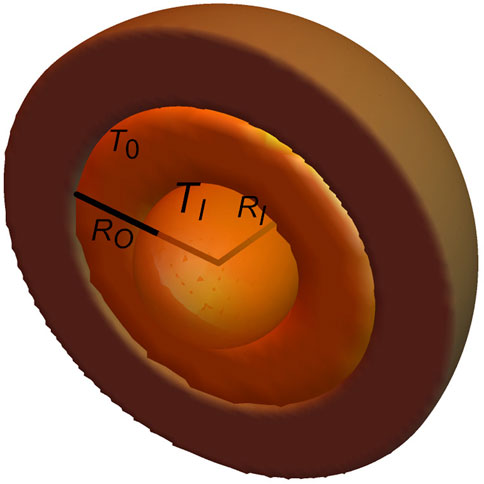
Figure 1. Typical interior of planets. This structure is common to both rocky and gaseous planets. The inner core radius is denoted by $R_I$, and the temperature at the beginning of the outer core is $T_I$. The outer core radius is $R_O$, and the temperature at the outer core-mantle boundary is $T_O$.

3 Results and discussion

We will now apply the theory developed in the previous section to the interiors of the planets in the solar system, except for Mars, which has a fossil magnetic field, and Venus, where accepted models are lacking, and the magnetic field strength is extremely small or nonexistent. We will evaluate the contribution to the magnetic fields of the planets with a conducting melted outer core, considering it as a degenerate Fermi gas in its electronic component. As we will see, the internal temperature of the planets and their satellites, and more in general of the other solar system objects, is clearly below Fermi’s temperature, $T_F={\epsilon }_F/k_B$, justifying the approximation.

The layer structure is common to all planets in our solar system, regardless of the component material of the several melted layers, metallic-ferrous in the case of rocky planets, and liquids with high conductivity in the case of giant planets (see Figure 1). Their fluid dynamics is likely a three-dimensional flow, as in the Earth case, where the inner core spins faster than the rest of the planet (Kerr, 2005), generating a three-dimensional velocity field. In Reference Bologna and Tellini (2014), the strength of the thermal contribution to the magnetic field was evaluated for Earth, Jupiter, and Ganymede, giving the order of magnitude of the observed values of the respective magnetic field at the surface.

We start the new discussion with Mercury, which has been explored in recent years by several space missions, particularly by the MESSENGER spacecraft that orbited Mercury for more than 4 years. Mercury has a radius of $R_P=2440$ km, an inner core radius $R_I\sim 1000$ km, an outer core radius $R_O\sim 2000$ km (Steinbrugge et al., 2021). The temperature at the beginning of the outer core is $T_I\sim 2800$ K, and the temperature at the outer core-mantle is $T_O\sim 2000$ K (Solomon et al., 2019; Edmund et al., 2022), the conductivity $\sigma \sim 10^4$ S/m (Manthilake et al., 2019). Assuming that the liquid outer core has a metallic behavior with a density $\rho \sim 7\times 10^3$ kg/m³ (Edmund et al., 2022; Christensen, 2006), then we may evaluate the Fermi’s energy ${\epsilon }_F\sim 1.10^{-17}$ J. Note: the corresponding Fermi’s temperature, $T_F={\epsilon }_F/k_B\sim 10^5$ K, amply justifies our assumption of a degenerate Fermi gas. Using the parameter values, we obtain the thermal magnetic field scale inside the planet

$B_T={\mu }_0\sigma \frac{k_B{T}_c}{e{\epsilon }_F}{k}_B\mathrm{\Delta }T\sim 0.035\hspace{0.17em}\mathrm{G}.(8)$

With sufficient accuracy, the magnetic field generated inside the planet is modeled as a dipole field. We infer that the dipole field decreases as $R^{-3}$, with $R$ the distance from the source, allowing us to estimate the corresponding surface field. Consequently, using the result of (Equation 8), we may write:

$B_S\sim B_T{\left(R_I/R_P\right)}^3\sim 0.0025\hspace{0.17em}\mathrm{G},(9)$

where $B_S$ is the surface field. The field magnitude given by (Equation 9) is in agreement with the measured field.

Following the planet order, after Earth, we come to Jupiter and its moon Ganymede, both explored during the 2000s by the Juno and Galileo spacecrafts. Using the approach presented in this paper, the theoretical magnitudes of the magnetic field of the two celestial bodies were evaluated in Reference Bologna and Tellini (2014). Here, we briefly outline Jupiter’s characteristics based on available recent data. In the region beginning at the metallic hydrogen layer, which extends for a fraction ranging from 0.6 to 0.8 times Jupiter’s radius, (Connerney et al., 2022; Moore et al., 2018; Militzer and Hubbard, 2024), the temperature is approximately $T\sim 10000$ K and $T\sim 8400$ K, respectively (Militzer and Hubbard, 2024; Hubbard, 1969). The density of metallic hydrogen in the outer core is estimated to be $\rho \sim 4\times 10^3{\mathrm{k}\mathrm{g}/\mathrm{m}}^3$ (Fortney and Nettelmann, 2009; French et al., 2012). This allows us to evaluate the Fermi energy as ${\epsilon }_F\sim 10^{-17}$ J. Finally, a recent estimation of the electrical conductivity gives the value $\sigma \sim 5\times 10^6$ S/m (Wicht et al., 2019). Using these parameter values, we obtain the thermal magnetic field scale inside the planet

$B_T={\mu }_0\sigma \frac{k_B{T}_c}{e{\epsilon }_F}{k}_B\mathrm{\Delta }T\sim 119\hspace{0.17em}\mathrm{G},(10)$

which corresponds to a surface field

$B_S\sim B_T{\left(R_I/R_P\right)}^3\sim 26\hspace{0.17em}\mathrm{G}.(11)$

The values given in Equations 10, 11 agree with the observations.

We now apply the same considerations to Saturn, which was explored over 2 decades by Cassini spacecraft (Dougherty et al., 2018; Cao et al., 2020). Using the data from (Cao et al., 2020) and references therein, the magnetic field at the planet’s surface is $0.2\lesssim B_S\lesssim 0.5$ G, the planet radius is $R_P\sim 60000$ km, with an inner core radius of $R_I\sim 15000$ km, and an outer core radius of $R_O\sim 30000$ km.

The metallic hydrogen region extends over a fraction of the planet, ranging from 0.6 to 0.75 times the planet radius (Cao et al., 2020). The temperature at the beginning of the conductive metallic region is approximately $T_I\sim 6000$ K, and the temperature at the outer core-mantle boundary is $T_O\sim 3000$ K (Helled, 2019). Saturn’s electrical conductivity is on the order of $\sigma \sim 10^5$ S/m (Cao et al., 2020), while the density of metallic hydrogen in the outer core is $\rho \sim 4\times 10^3$ kg/m³ (Fortney and Nettelmann, 2009; French et al., 2012). This allows us to evaluate the Fermi energy, ${\epsilon }_F\sim 10^{-17}$ J. The corresponding Fermi’s temperature, $T_F={\epsilon }_F/k_B\sim 7\times 10^5$ K, again amply justifies our zero temperature Fermi statistics assumption. Using the parameter values, we obtain the thermal magnetic field scale inside the planet

$B_T={\mu }_0\sigma \frac{k_B{T}_c}{e{\epsilon }_F}{k}_B\mathrm{\Delta }T\sim 2.7\hspace{0.17em}\mathrm{G},(12)$

where we used the intermediate value $\sigma \sim 5\times 10^5$ for the conductivity, and corresponding to a surface field

$B_S\sim B_T{\left(R_I/R_P\right)}^3\sim 0.6\hspace{0.17em}\mathrm{G}.(13)$

The values given in Equations 12, 13 agree with the observations.

We now apply the same considerations to the planets Uranus and Neptune. Despite data obtained from recent spatial missions, the models of the interiors of Uranus and Neptune remain poorly understood and still affected by significant uncertainty (see (Helled et al., 2011; Helled and Fortney, 2020; Helled et al., 2020; Neuenschwander et al., 2024) for reviews). It is widely accepted that both planets are rich in water or water-like components and heavy elements, though the specific concentrations vary significantly depending on the model. Several studies propose models in which the interiors of these planets include a layer of metallic fluid hydrogen, which is considered to be the primary driver of their planetary dynamo. However, a detailed analysis of these hypothesis is beyond the scope of this Brief. For our analysis, we rely on the model presented in Reference Nellis (2017). In particular, we emphasize that our conjecture regarding the contribution of the Seebeck current to the planetary magnetic field requires only the presence of a fluid with high electrical conductivity to validate our approximation, which is based on the ideal degenerate Fermi gas. In other words, the presence of a conducting fluid is essential, but it does not necessarily need to be metallic fluid hydrogen.

Regarding Equation 7, the physical parameters of the two planets exhibit similar values. There is a common agreement that $\sigma \sim 10^5$ S/m. Such a region is modeled to extend to approximately 0.9 $R_p$, while the magnetic field is thought to be generated between 0.5 $R_P$ and 0.7 $R_P$. The temperature at the beginning of the outer core is approximately $T_I\sim 3000$ K, while the temperature at the outer core-mantle boundary is $T_O\sim 1500$ K. The density is estimated $\rho \sim 10^3$ kg/m³ (Chau et al., 2011; Nellis, 2017) giving a Fermi energy ${\epsilon }_F\sim 4\times 10^{-18}$ J. The corresponding Fermi temperature, $T_F={\epsilon }_F/k_B\sim 3\times 10^5$ K, fully supports our assumption. Inside the planets, we have

$B_T={\mu }_0\sigma \frac{k_B{T}_c}{e{\epsilon }_F}{k}_B\mathrm{\Delta }T\sim 1.62\hspace{0.17em}\mathrm{G},(14)$

where we used the intermediate value $R_I\sim 0.6R_P$ and corresponding to a surface field

$B_S\sim B_T{\left(R_I/R_P\right)}^3\sim 0.35\hspace{0.17em}\mathrm{G}.(15)$

The values given in Equations 14, 15 agree with the observations.

The results of our discussion are summarized in Table 1, containing all the relevant physical parameters of the planets, and Table 2, where we compare the observed values of the magnetic field and the values given by the thermal contribution.

Table 1

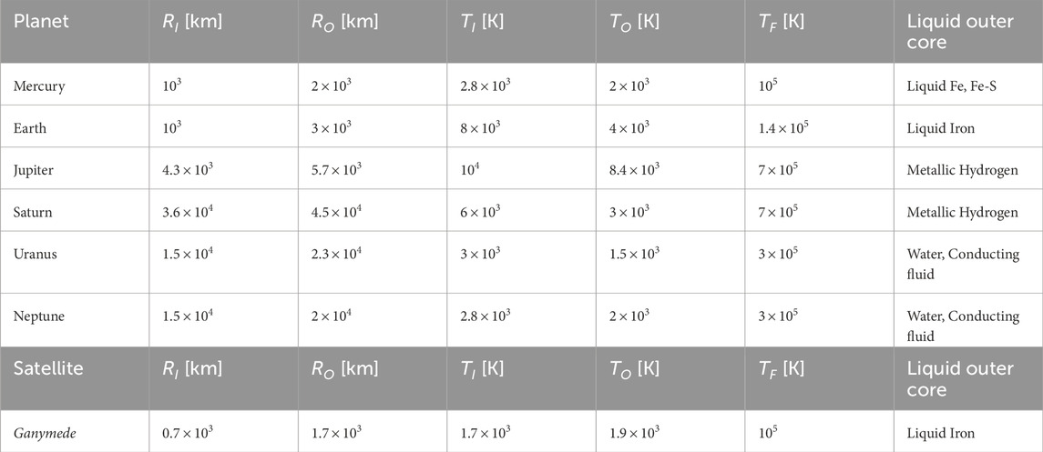
Table 1. Planetary physical parameters (including the satellite Ganymede in italics to stress that it is not a planet) for the evaluation of $B_T$. In the second column is the inner core radius. In the third, is the outer core radius. In the fourth, the temperature at the beginning of the outer core. In the fifth, the temperature at the outer core-mantle. In the sixth, the Fermi temperature corresponding to the density of the liquid outer core. Finally, in the seventh, the composition of the liquid outer core.

Table 2

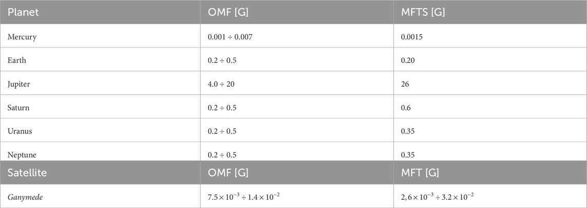
Table 2. Comparison between the observed values of the magnetic field and the values given by the thermal contribution. In the second column the Observed Magnetic Field at the surface (OMF) and in the third the Magnetic Field from thermal current at the surface (MFTS), Equation 7. The values of the Earth and Jupiter magnetic fields, as well as the magnetic field of the Jupiter satellite Ganymede (in italics to stress that it is not a planet), have been evaluated in Reference Bologna and Tellini (2014).

The data reported in Table 2 are consistent with the conjecture presented in this paper. The assumption of a thermal current density generated by the Seebeck effect, resulting from a thermal gradient between the inner and outer core of a planet, demonstrates its capability to encompass a relevant part of the magnitude of the planetary magnetic field. The presence of a thermal gradient and the essential condition that the degenerate Fermi gas approximation is a well-founded hypothesis for describing the conducting fluid behavior in the planet form the basis of our discussion. This novel approach offers a new perspective for discussing magnetic fields generated by planets.

4 Conclusion

In this paper, we developed our conjecture that thermal density currents (Seebeck effect) can significantly contribute to the magnetic fields of celestial bodies, specifically the planets of our solar system. However, our analysis does not extend to Mars or Venus because Mars’ magnetic field is considered a fossil magnetic field, and our knowledge of the interiors of Venus is limited. We evaluated the thermal contribution of the magnetic field using the magnitude scale $B_T={\mu }_0\sigma k_B^2{T}_c\mathrm{\Delta }T/(e{\epsilon }_F)$ for Mercury, Earth, Jupiter (and Ganymede), Saturn, Uranus, and Neptune. The results are presented in Table 2, where we compare our findings with magnetic field measurements from various spatial missions, demonstrating a consistent agreement with the observed values.

While we did not face the challenge of solving the magnetohydrodynamic equations, we focused on the magnitude order of the magnetic field and the physic associated. An important feature of the magnetic scaling in our conjecture is its relation with the Fermi-Dirac statistic, which we applied to the fluid of the outer cores of the planets. Our research shows that a thermal current density generated by the Seebeck effect can significantly contribute to the intensity of the planetary magnetic field.

Data availability statement

The original contributions presented in the study are included in the article/supplementary material, further inquiries can be directed to the corresponding author.

Author contributions

MB: Conceptualization, Investigation, Writing–original draft, Writing–review and editing. KC: Conceptualization, Investigation, Writing–original draft, Writing–review and editing. BT: Conceptualization, Investigation, Writing–original draft, Writing–review and editing.

Funding

The author(s) declare financial support was received for the research, authorship, and/or publication of this article. K.J.C. and MB acknowledge financial support from UTA Mayor project No 8740-24.

Conflict of interest

The authors declare that the research was conducted in the absence of any commercial or financial relationships that could be construed as a potential conflict of interest.

Publisher’s note

All claims expressed in this article are solely those of the authors and do not necessarily represent those of their affiliated organizations, or those of the publisher, the editors and the reviewers. Any product that may be evaluated in this article, or claim that may be made by its manufacturer, is not guaranteed or endorsed by the publisher.

References

Bologna, M., and Tellini, B. (2010). Generating a magnetic field by a rotating plasma. Europhys. Lett. 91, 45002–45006. doi:10.1209/0295-5075/91/45002

CrossRef Full Text | Google Scholar

Bologna, M., and Tellini, B. (2014). Analytical estimation of the scale of earth-like planetary magnetic fields. Earth, Moon, Planets 113, 99–107. doi:10.1007/s11038-014-9447-5

CrossRef Full Text | Google Scholar

Cao, H., Dougherty, M. K., Hunt, G. J., Provan, G., Cowley, S. W., Bunce, E. J., et al. (2020). The landscape of saturn’s internal magnetic field from the cassini grand finale. Icarus 344, 113541. doi:10.1016/j.icarus.2019.113541

CrossRef Full Text | Google Scholar

Chau, R., Hamel, S., and Nellis, W. J. (2011). Chemical processes in the deep interior of uranus. Nat. Commun. 2, 203–205. doi:10.1038/ncomms1198

PubMed Abstract | CrossRef Full Text | Google Scholar

Christensen, U. (2006). A deep dynamo generating mercury’s magnetic field. Nature 48, 1056–1058. doi:10.1038/nature05342

PubMed Abstract | CrossRef Full Text | Google Scholar

Christensen, U. R. (2010). Dynamo scaling laws and applications to the planets. Space Sci. Rev. 152, 565–590. doi:10.1007/s11214-009-9553-2

CrossRef Full Text | Google Scholar

Christensen, U. R., Holzwarth, V., and Reiners, A. (2018). Energy flux determines magnetic field strength of planets and stars. Nature 457, 167–169. doi:10.1038/nature07626

PubMed Abstract | CrossRef Full Text | Google Scholar

Connerney, J. E. P., Timmins, S., Oliversen, R. J., Espley, J. R., Joergensen, J. L., Kotsiaros, S., et al. (2022). A new model of jupiter’s magnetic field at the completion of juno’s prime mission. J. Geoph. Res. Planets 127, 1–15. doi:10.1029/2021JE007055

CrossRef Full Text | Google Scholar

Dougherty, M. K., Cao, H., Khurana, K. K., Hunt, G. J., Provan, G., Kellock, S., et al. (2018). Saturn’s magnetic field revealed by the cassini grand finale. Science 362, eaat5434–53. doi:10.1126/science.aat5434

PubMed Abstract | CrossRef Full Text | Google Scholar

Edmund, E., Morard, G., Baron, M. A., Rivoldini, A., Yokoo, S., Bacoota, S., et al. (2022). The fe-fesi phase diagram at mercury core conditions. Nat. Commun. 13, 387 1–9. doi:10.1038/s41467-022-27991-9

CrossRef Full Text | Google Scholar

Fortney, J. J., and Nettelmann, N. (2009). The interior structure, composition, and evolution of giant planets. Space Sci. Rev. 152, 423–447. doi:10.1007/s11214-009-9582-x

CrossRef Full Text | Google Scholar

French, M., Becker, A., Lorenzen, W., Nettelmann, N., Bethkenhagen, M., Wicht, J., et al. (2012). Ab initio simulations for material properties along the jupiter adiabat. Astrophysical J. Suppl. Ser. 202, 5–1. doi:10.1088/0067-0049/202/1/5

CrossRef Full Text | Google Scholar

Helled, R. (2019). The interiors of jupiter and saturn. Oxf. Res. Encycl. Planet. Sci. doi:10.1093/acrefore/9780190647926.013.175

CrossRef Full Text | Google Scholar

Helled, R., Anderson, J. D., Podolak, M., and Schubert, G. (2011). Interior models of uranus and neptune. Astrophysical J. 726, 15. doi:10.1088/0004-637X/726/1/15

CrossRef Full Text | Google Scholar

Helled, R., and Fortney, J. J. (2020). The interiors of uranus and neptune: current understanding and open questions. Philosophical Trans. R. Soc. A 378, 20190474–20190491. doi:10.1098/rsta.2019.0474

PubMed Abstract | CrossRef Full Text | Google Scholar

Helled, R., Nettelmann, N., and Guillot, T. (2020). Uranus and neptune: origin, evolution and internal structure. Space Sci. Rev. 216, 38-1–38-26. doi:10.1007/s11214-020-00660-3

CrossRef Full Text | Google Scholar

Hubbard, W. (1969). Thermal models of jupiter and saturn. Astrophys. J. 155, 333–344. doi:10.1086/149868

CrossRef Full Text | Google Scholar

Kerr, R. A. (2005). Earth’s inner core is running a tad faster than the rest of the planet. Science 309, 1313. doi:10.1126/science.309.5739.1313a

PubMed Abstract | CrossRef Full Text | Google Scholar

Landau, L., and Lifshitz, E. (1981a). Electrodynamics of continuous media. Oxford: Pergamon Press.

Google Scholar

Landau, L., and Lifshitz, E. (1981b). Physical kinetics. Oxford: Pergamon Press.

Google Scholar

Manthilake, G., Chantel, J., Monteux, J., Andrault, D., Bouhifd, M. A., Bolfan Casanova, N., et al. (2019). Thermal conductivity of fes and its implications for mercury’s long-sustaining magnetic field. J. Geophys. Res. Planets 124, 2359–2368. doi:10.1029/2019JE005979

CrossRef Full Text | Google Scholar

Militzer, B., and Hubbard, W. B. (2024). Study of jupiter’s interior: Comparison of 2, 3, 4, 5, and 6 layer models. Icarus 411, 115955. doi:10.1016/j.icarus.2024.115955

CrossRef Full Text | Google Scholar

Moore, K. M., Yadav, R. K., Kulowski, L., Cao, H., Bloxham, J., Connerney, J. E. P., et al. (2018). A complex dynamo inferred from the hemispheric dichotomy of jupiter’s magnetic field. Nature 561, 76–78. doi:10.1038/s41586-018-0468-5

PubMed Abstract | CrossRef Full Text | Google Scholar

Nellis, W. J. (2017). Magnetic fields of uranus and neptune: metallic fluid hydrogen. J. Phys. Conf. Ser. 950, 042046. doi:10.1088/1742-6596/950/4/042046

CrossRef Full Text | Google Scholar

Neuenschwander, B. A., Müller, S., and Helled, R. (2024). Uranus’s complex internal structure. A&A 684, A191-1–A191-14. doi:10.1051/0004-6361/202348028

CrossRef Full Text | Google Scholar

Reiners, A., and Christensen, U. R. (2010). A magnetic field evolution scenario for brown dwarfs and giant planets. A& 522, A13–A17. doi:10.1051/0004-6361/201014251

CrossRef Full Text | Google Scholar

Solomon, S. C., Nittler, L. R., and Anderson, B. J. (2019). Mercury the View after MESSENGER Cambridge: Cambridge University Press.

Google Scholar

Steinbrugge, G., Dumberry, M., Rivoldini, A., Schubert, G., Cao, H., Schroeder, D. M., et al. (2021). Challenges on mercury’s interior structure posed by the new measurements of its obliquity and tides. Geophys. Res. Lett. 48, 1–10. doi:10.1029/2020GL089895

CrossRef Full Text | Google Scholar

Stevenson, D. J. (1983). Planetary magnetic fields. Rep. Prog. Phys. 46, 555–620. doi:10.1088/0034-4885/46/5/001

CrossRef Full Text | Google Scholar

Stevenson, D. J. (2010). Planetary magnetic fields: achievements and prospects. Space Sci. Rev. 152, 651–664. doi:10.1007/s11214-009-9572-z

CrossRef Full Text | Google Scholar

Toepfer, S., Narita, Y., and Schmid, D. (2022). Reconstruction of the interplanetary magnetic field from the magnetosheath data: a steady-state approach. Front. Phys. 10, 1050859. doi:10.3389/fphy.2022.1050859

CrossRef Full Text | Google Scholar

Wicht, J., Gastine, T., Duarte, L. D. V., and Dietrich, W. (2019). Dynamo action of the zonal winds in jupiter. A&A 629, A125-1–A125-11. doi:10.1051/0004-6361/201935682

CrossRef Full Text | Google Scholar