Feature importance analysis of solar flares and prediction research with ensemble machine learning models

Solar flares, as intense solar eruptive events, have a profound impact on space weather, potentially disrupting human activities like spaceflight and communication. Hence, identify the key factors that influence the occurrence of solar flares and accurate forecast holds significant research importance. Considering the imbalance of the flare data set, three ensemble learning models (Balanced Random Forest (BRF), RUSBoost (RBC), and NGBoost (NGB)) were utilized, which have gained popularity in statistical machine learning theory in recent years, combined with imbalanced data sampling techniques, to classify and predict the labels representing flare eruptions in the test set. In this study, these models were used to classify and predict flares with a magnitude $\ge$ C- and M-class, respectively. After obtaining the feature importance scores of each model, a comprehensive feature importance ranking was derived based on the ranking. The main results are as follows: (1) For the prediction of flares $\ge$ C- and M-class, the best-performing model achieved a Recall of $\sim 0.76$, $\sim 0.88$ and a ${\mathrm{T}}_{\mathrm{s}\mathrm{s}}$ score of $\sim 0.65$, $\sim 0.78$ on the test set, respectively. These are relatively high scores for model performance evaluation metrics. (2) The importance scores of each feature under different evaluation metrics and the comprehensive importance ranking can be directly obtained through the model without the need for additional feature analysis tools. Using this ranking to reduce the dimensionality of the data set for the three main models, similar or better classification results can be achieved using only about half of the original features. (3) Our results demonstrate the mean photospheric magnetic free energy (MEANPOT), the time decay value based on the magnitudes of all previous flares (Edec), and the total unsigned current helicity (TOTUSJH). They are the three quantities that have the most significant relationship with solar flares, which include free energy, twist degree, and the historical information of flare occurrences, respectively. Besides, analyzing the feature parameters of four different active regions, we find that the geographical information of the flare occurrence is an important factor. The object of this work is to provide prediction methods for imbalanced data as well as feature importance ranking methods.

1 Introduction

Solar flares are one of the intense solar eruptive activities, manifesting as bright chromospheric ribbons and hot coronal loops on the Sun, releasing a large amount of energy, which typically lasts from a few minutes to several hours. Based on the magnitude of energy released, solar flares are classified into different levels, commonly using X-ray radiation intensity as the criterion. The flare levels range from A-, B-, C-, M-to X-class, with higher levels indicating greater energy release. High-level solar flares are often accompanied by coronal mass ejections (CMEs) (Jing et al., 2004; Yan et al., 2011; Chen, 2011; Webb and Howard, 2012), which can significantly impact space weather, thereby posing hazards to human activities such as communications and spaceflight (Baker et al., 2004). Therefore, analyzing variables related to solar flares and further establishing practical prediction models for solar flares is of great practical significance.

Currently, the primary methods for correlation analysis and prediction of solar flares encompass traditional statistical models (Gallagher et al., 2002; Bloomfield et al., 2012; Mason and Hoeksema, 2010), physical numerical models (Feng, 2020), and machine learning models. Traditional statistical models summarize the relationships between observed quantities and those to be predicted, deriving corresponding statistical distribution models. While these methods are simple and fast, they lack accuracy. Physical numerical models, which predict through numerical calculations simulating the generation mechanism of solar flares, are constrained by the incomplete understanding of solar flare triggering mechanisms. In recent years, due to the rapid advancement of computing capabilities, artificial intelligence algorithms have been introduced for predicting solar flares and addressing other space weather issues. The progress in machine learning technology has yielded efficient and accurate classification and correlation analysis algorithms, including Support Vector Machines (SVM) (Li et al., 2007; Bobra and Couvidat, 2015; Nishizuka et al., 2017), Random Forest (RF) (Breiman, 2001; Liu et al., 2017), XGBoost (XGB) (Sharma, 2017; He, 2021), and Long Short-Term Memory (LSTM) (Wang et al., 2020; Liu et al., 2019). These algorithms have found wide application in the analysis and research of space physics data. Concurrently, the development of solar activity observation techniques and instruments has provided extensive data on solar flares and magnetograms (Schou et al., 2012), serving as crucial sample support for the application of machine learning algorithms. Essentially, predicting solar flares boils down to a classification and prediction problem in machine learning. Therefore, machine learning algorithms can be leveraged to analyze large samples and identify variables that significantly impact solar flares. These selected variables can then be used to train classification and prediction models, enabling data-driven forecasting of solar flares.

In the realm of solar flare analysis and prediction utilizing machine learning techniques, scholars have extensively explored various methodologies. Song et al. (2009) constructed an ordinal logistic regression model based on three predictive parameters to forecast the likelihood of X-, M-, and C-class flares occurring within a 24-h window. Boucheron et al. (2015) developed an SVM regression model, incorporating 38 features that characterize the magnetic complexity of the photospheric magnetic field, to predict flare magnitude and timing. Wang et al. (2020) applied the LSTM method to predict the maximum flare class within the next 24 h, using a data set comprised of 20 SHARP parameters from the Joint Science Operations Center’s active region data spanning from 2010 to 2018. Huang et al. (2018) and Wang et al. (2023) harnessed the power of convolutional neural networks (CNN) for image processing to make predictions. While these studies primarily focus on prediction outcomes, they do not delve into the analysis of feature importance. Bobra and Couvidat (2014) merged a vast data set of vector magnetograms with the SVM algorithm to forecast X-class and M-class solar flares. They screened 25 parameters and retained the top 13, which include TOTUSJH, TOTBSQ, TOTPOT, TOTUSJZ, ABSNJZH, SAVNCPP, USFLUX, AREA-ACR, TOTFZ, MEANPOT, R-VALUE, EPSZ, and SHRGT. The physical implications of these parameters are detailed in Table 1. Building on the findings of Bobra and Couvidat (2014), Liu et al. (2017) employed the first 13 parameters and the RF method to predict flare occurrences within a 24-hour period. Liu et al. (2019) established three LSTM networks tailored for three classes of solar flares, marking the inaugural application of LSTM in solar flare prediction. Utilizing a time series data set featuring 25 magnetic field parameters and 15 flare historical parameters, they surpassed other machine learning methods in label prediction performance. Notably, they discovered that using a subset of 14–22 of the most significant parameters yielded better prediction results than utilizing all 40 parameters concurrently. He (2021) adopted the XGB method to scrutinize the importance of diverse physical parameters in the SDO/HMI SHARP data, subsequently establishing an LSTM network based on the selected features. Ran et al. (2022) investigated the continuous eruptions of flares using 16 SHARP parameters to pinpoint the most pertinent ones. By computing correlation coefficients and variable importance scores derived from the NGB algorithm, they pinpointed eight parameters that are most closely associated with flares within the same active region. Sinha et al. (2022) conducted a feature importance ranking with 19 features, concluding that magnetic properties such as total current helicity (TOTUSJH), total vertical current density (TOTUSJZ), total unsigned flux (USFLUX), sum of unsigned flux near PIL (R-VALUE), and total absolute twist (TOTABSTWIST) are the top-performing flare indicators. Lastly, Deshmukh et al. (2023) analyzed 20 features, encompassing both physics-based and shape-based attributes, and found that shape-based features are not significant indicators.

Table 1

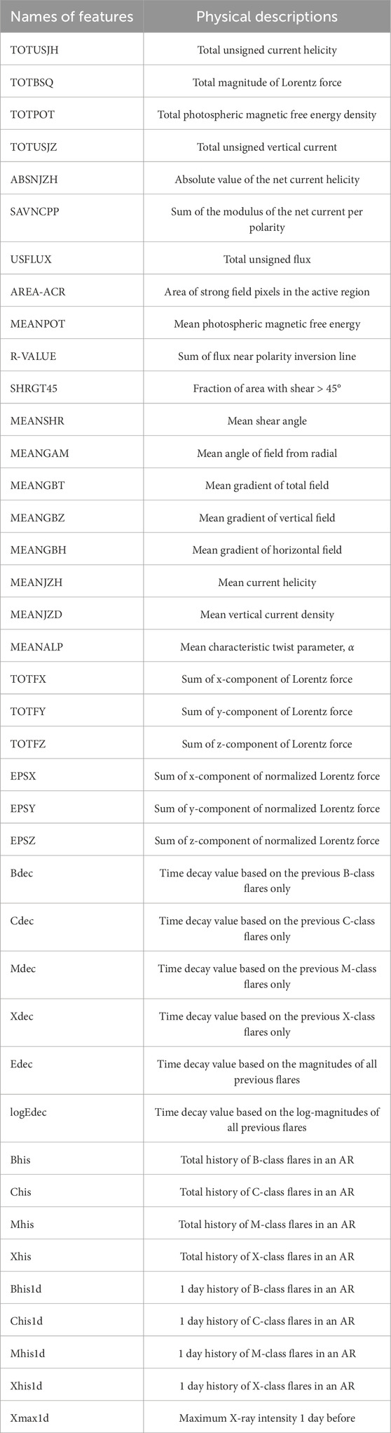
Table 1. Names of 40 features and their physical descriptions.

Currently, the triggering mechanism of solar flares remains incompletely understood (Priest and Forbes, 2002). By applying machine learning algorithms to solar flare data for correlation analysis, we can obtain importance scores for various variables, which quantify the influence of corresponding physical quantities on solar flares. These scores serve as a valuable reference for elucidating the flare triggering mechanism. Furthermore, selecting variables with higher importance scores aids in simplifying the classification model, mitigating over-fitting, and enhancing the efficiency and accuracy of the classification prediction model. In summary, leveraging machine learning algorithms to analyze correlations between solar flare and magnetic field data in solar active regions, and subsequently utilizing these insights for solar flare prediction, holds considerable practical significance and theoretical value.

The structure of this study is organized as follows: In Section 2, we introduce the data set and define the criteria for Positive and Negative Samples. Section 3 presents the theoretical foundation of three models, elaborating on the theory behind imbalanced classification model algorithms and comparing the strengths and weaknesses of different algorithms from a theoretical standpoint. In Section 4, we delve into feature importance analysis and model evaluation metrics. Furthermore, we select four solar active regions to examine and compare their differences in feature importance. Section 5 presents the results and discussions. Lastly, we provide a summary in Section 6.

2 Data acquisition and preprocessing

Currently, commonly used observation data includes the magnetic field characteristic data of the photosphere in solar active regions and flare historical data. The former is considered to be closely related to solar flares (Shibata and Magara, 2011; Priest and Forbes, 2002), while the latter is widely used in machine learning methods involving time series. The flare prediction data set used in this article is primarily based on the paper “Predicting Solar Flares Using a Long Short-term Memory Network” (Liu et al., 2019). The data sources include the SHARP data set created by the SDO/HMI team and its derivative cgem. Lorentz data set (Fisher et al., 2012; Chen et al., 2019) as well as the GOES X-ray flare catalog from the NCEI (National Centers for Environmental Information) covering the period from May 2010 to May 2018. After removing missing values, feature construction, labeling, and standardization, 2,34,476 flare samples $\ge$ C-class and above were selected. Among them, 1,27,709 samples were used for the training set, 36,953 for the validation set, and 69,814 for the test set. For flares $\ge$ M-class, there were a total of 155,739 samples, with 84,577 samples in the training set, 26,473 in the validation set, and 44,689 in the test set. The sampling interval for each sample is 1 h, and each sample includes 40 features used for flare prediction. These features include 25 physical parameters describing magnetic field characteristics and 15 parameters related to flare historical data. The names of features and their physical descriptions are shown in Table 1.

Jonas et al. (2018) pointed out that historical flare data plays a significant role in flare prediction. This historical data primarily includes six time-decay parameters related to historical flare data: Bdec, Cdec, Mdec, Xdec, Edec, and logEdec, as well as eight flare count parameters. The specific calculation formulas are as follows.

$\mathrm{B}\mathrm{d}\mathrm{e}\mathrm{c}\left({\mathrm{X}}_{\mathrm{t}}\right)={\displaystyle \sum _{f_i\in F_B}}{e}^{\frac{t-t\left(f_i\right)}{\tau }},(\mathrm{1a})$

$\mathrm{C}\mathrm{d}\mathrm{e}\mathrm{c}\left({\mathrm{X}}_{\mathrm{t}}\right)={\displaystyle \sum _{f_i\in F_C}}{e}^{\frac{t-t\left(f_i\right)}{\tau }},(\mathrm{1b})$

$\mathrm{M}\mathrm{d}\mathrm{e}\mathrm{c}\left({\mathrm{X}}_{\mathrm{t}}\right)={\displaystyle \sum _{f_i\in F_M}}{e}^{\frac{t-t\left(f_i\right)}{\tau }},(\mathrm{1c})$

$\mathrm{X}\mathrm{d}\mathrm{e}\mathrm{c}\left({\mathrm{X}}_{\mathrm{t}}\right)={\displaystyle \sum _{f_i\in F_X}}{e}^{\frac{t-t\left(f_i\right)}{\tau }},(\mathrm{1d})$

$\mathrm{E}\mathrm{d}\mathrm{e}\mathrm{c}\left({\mathrm{X}}_{\mathrm{t}}\right)={\displaystyle \sum _{f_i\in F}}E\left(f_i\right)e^{\frac{t-t\left(f_i\right)}{\tau }},(1e)$

$\log \mathrm{E}\mathrm{d}\mathrm{e}\mathrm{c}\left({\mathrm{X}}_{\mathrm{t}}\right)={\displaystyle \sum _{f_i\in F}}\log \left(E\left(f_i\right)\right)e^{\frac{t-t\left(f_i\right)}{\tau }}.(\mathrm{1f})$

In the above formulas (Equations 1a–1f), ${\mathrm{X}}_{\mathrm{t}}$ represents the observed sample data at time $t$. $F_B$, $F_C$, $F_M$, and $F_X$ denote the sets of all B-, C-, M- and X-class flares that occurred in the current solar active region before time $t$. $t(f_i)$ represents the time point at which flare $f_i$ occurred, and $\tau$ is the time decay constant, set to 12. $F$ represents the set of all flares of any class that occurred in the current solar active region before time $t$, and $E(f_i)$ represents the size (or energy) of flare $f_i$. Observing the above formulas, for the four parameters Bdec, Cdec, Mdec, and Xdec, flares that occurred closer to the observation time $t$ have a greater influence on the respective parameters. Flares that occurred further away from the observation time are also included in the respective parameters, but have a smaller impact on the parameter values. In the calculation of Edec and logEdec, not only the influence of the flare occurrence time on the parameter values is considered, but also the different impacts of flare class sizes on the parameter values. By incorporating these six time-decay parameters and an additional nine parameters related to flare counts and X-ray maxima in the active region, the time series nature of flare data is fully considered.

The prediction target of this study is to forecast whether $\ge$ C-class or M-class solar flare will occur in a specific solar active region within the next 24 h. Essentially, this is a binary classification problem, and thus the data needs to be appropriately labeled. The labeling method is as follows: As shown in Figure 1, each grid represents a 1 h time interval, which is also the sampling interval of the samples. Samples taken within the 24 h prior to the occurrence of a solar flare of or above the specified class are labeled as Positive i.e., positive samples, while the remaining samples are labeled as Negative, i.e., negative samples. The hour in which the flare actually occurs is excluded from the data set. After labeling, the positive and negative sample ratios of the prediction data sets for flares $\ge$ C-class and $\ge$ M-class (hereinafter referred to as the C data set and the M data set) are presented in Table 2 and Table 3, respectively. As can be observed from the tables, the ratio of positive and negative samples is imbalanced, with the proportion of positive samples being far lower than that of negative samples. This imbalance is even more pronounced on the M data set. Most ARs provide around 200 samples, with a few exceeding 300.

Figure 1

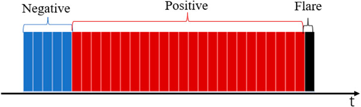
Figure 1. The labeling method for positive and negative samples.

Table 2

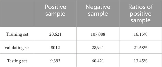
Table 2. Positive and negative sample ratios of C data set.

Table 3

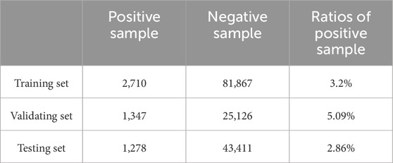
Table 3. Positive and negative sample ratios of M data set.

3 Introduction of three ensemble models used

Ensemble model uses the Boosting or Bagging algorithm to integrate some single models, which makes the algorithm powerful. These integrated single models are also called basic estimators. The main idea of the ensemble algorithm is to use basic estimators to accomplish the preliminary learning of the data set, and adjust the weight of each sample event according to the learning results. The weight of the correct sample event will be reduced in the next round of learning, while that of the wrong sample event will be increased in the next round of learning, and then the data set with adjusted weight will be re-trained by the next estimator. Finally, the weighted average of the errors of different basic estimators is taken as the final output result of the ensemble model. In this study, three ensemble learning prediction models were employed: BRF, RBC, and NGB, which are designed to handle imbalanced data. we compared the performance of several mainstream machine learning methods those have outstanding performance in this or other fields, including three kinds of ensemble models.

Random Forest algorithm was proposed by Breiman (2001), which is an ensemble learning model based on bagging and has strong generalization. The commonly used base learner of Random Forest algorithm is decision tree (Berk, 2016). The training set of each decision tree is obtained through bootstrap sampling, and the criterion for selecting the optimal splitting feature of its nodes is the Gini index. However, the traditional Random Forest algorithm has limitations in handling imbalanced classification problems. Since its training goal is to minimize the overall classification error rate, it tends to pay more attention to the classification results of the majority class and ignores the classification results of the minority class. In addition, during the generation of the training set for each decision tree, there is a possibility that only a few positive samples or even no positive samples are present in the sample subset obtained by bootstrap sampling. The decision trees trained by these sample subsets cannot learn the characteristics of positive samples. The above two points lead to the low accuracy of the Random Forest algorithm in predicting the minority class. To improve the performance of Random Forest algorithm in imbalanced classification problems, Chen and Breiman (2004) proposed Balanced Random Forest. Compared with the traditional Random Forest, Balanced Random Forest adds a down-sampling step to the bootstrap sampling, ensuring that the training set of each decision tree is balanced. By adding down sampling to the bootstrap sampling process, Balanced Random Forest ensures that each training subset is balanced. The base learner can fully learn the characteristics of the minority class samples, and since different base learners have different down sampling subsets for the majority class, the information of the majority class samples can also be learned by different base learners, alleviating the loss of information of the majority class samples in down sampling and effectively improving the classification effect on the minority class samples.

The RUSBoost algorithm, proposed by Seiffert et al. (2010), is a combination of RUS (Random under sampling) and AdaBoost. It further enhances AdaBoost’s predictive capabilities for imbalanced data through random downsampling. Although the introduction of sample weights in the AdaBoost algorithm effectively alters the distribution of the data set, the basis for weight updates remains the overall error rate of the base learner during the iterative process, thus increasing the focus on misclassified samples. However, for imbalanced data, the majority class samples still tend to dominate among the misclassified samples, and the issue of the model’s low attention to the minority class in imbalanced data remains unresolved. The RUSBoost algorithm addresses this by incorporating a random under sampling step before each iteration of AdaBoost to generate a balanced training set for that iteration, which is obtained by randomly under sampling the original training set. The random under sampling incorporated at the beginning of each iteration ensures that the training set for each base learner is a balanced data set, addressing the issue of low attention to minority class samples. Additionally, it retains the weight boosting of misclassified samples in the AdaBoost algorithm, making RUSBoost achieve better results in imbalanced data classification.

NGBoost (Duan et al., 2020) is a Boosting algorithm based on natural gradients. Unlike other Boosting methods used for classification or regression, NGBoost does not directly predict categorical labels or regression values. Instead, it predicts the parameters of the conditional distribution to which the samples belong, thereby obtaining the probability density of the target variable. The benefits of using natural gradients for parameter learning are obvious. Natural gradients take divergence as an approximate distance metric, representing the steepest direction of ascent in Riemannian space, and remain invariant to parameterization, making the optimization process unaffected by parameterization. In classification problems, NGBoost directly predicts probability distributions, which not only allows us to obtain predictions for label values but also the probabilities corresponding to different label values. This enables us to set appropriate probability thresholds based on practical requirements to handle imbalanced classification issues. The NGBoost algorithm boasts three main advantages. Firstly, it can predict conditional distributions, which provides more flexibility in utilizing predicted outputs in both classification and regression problems. While the type of distribution to be fitted needs to be specified beforehand, there are numerous options to choose from, making it applicable in areas such as counting, survival prediction, and data censoring. Secondly, it exhibits stability in multi-parameter boosting, where natural gradients are used as approximate distances, enabling various parameters to converge together at similar rates during the boosting process. Thirdly, it possesses strong parameterization capabilities, which also benefit from the invariance of natural gradients to parameterization, allowing for the fitting of various distributions and their parameters. However, the NGBoost algorithm also has the disadvantage of high computational cost. For each parameter, a set of base learners must be trained, and the natural gradient of each sample must be calculated. When the fitted distribution has a large number of parameters and the data set contains many samples, the computational cost increases significantly.

4 Feature importance ranking and model evaluation metrics

Feature selection is based on the importance ranking of the features and some thresholds. According to the correlation between the label and features or the contribution of the features in training, the importance of each feature is ranked by a certain criterion (scores obtained based on the contribution of features to model performance), and then the features with weak correlation are eliminated by setting a threshold. Feature selection can not only reduce the computational cost for large multivariate sample data sets, but also eliminate the interference of some redundant features to the prediction results (Yang et al., 2023). The crucial features selected out will be used for the machine learning model in the training and testing, so the feature selection results will directly influence the final prediction results of the model. The information gain method is a built-in method of ensemble models. It combines the learning process of the model to rank the features and can help select the important features that closely match the model. The information gain method of decision tree model is a typical representative of this kind of methods. The feature selection function of the ensemble model itself is based on the principle of Embedded Methods given the differences in calculation methods for variable importance among various models, the resulting variable importance scores also vary. We combined the variable importance results from three models. After obtaining the importance scores of each model, we take the average score of the three models, and based on the comprehensive score, we obtain the final ranking of each feature.

In binary classification problems, the most commonly used evaluation metrics are error rate and accuracy. The error rate is calculated by dividing the number of misclassified samples by the total number of samples, while the accuracy is calculated by dividing the number of correctly classified samples by the total number of samples. The error rate describes how many samples in the data set are misclassified by the model, while the accuracy describes how many samples in the data set are correctly classified by the model. These metrics that focus on the overall classification effect are appropriate as model evaluation metrics in data sets with balanced or approximately balanced positive and negative samples.

However, for imbalanced data sets, the effectiveness of using error rate and accuracy as evaluation metrics is not good (He and Garcia, 2009). Because these two metrics focus on the overall classification effect and tend to overlook the classification results on minority classes. An extreme example can be given: if an imbalanced data set has 1 positive sample and 99 negative samples, and a prediction model is established that predicts the label value $y$ as negative regardless of the observed value $x$, then the error rate of this model on this imbalanced data set is $1\%$, and the accuracy is $99\%$, which seems to be a very good result. However, such a prediction model is meaningless. The reason is that the proportion of minority class samples is low, and the model only needs to improve the prediction effect on the majority class samples as much as possible. Even if a large number of minority class samples are predicted incorrectly, the impact on the overall prediction metrics is still small. However, the model trained in this way has poor prediction performance on minority class samples and has no practical application value. To solve this problem, more sophisticated evaluation metrics such as recall, precision, ${\mathrm{T}}_{\mathrm{s}\mathrm{s}}$ score, and ${\mathrm{F}}_{\mathrm{1}}$ score need to be used.

First, we need to introduce the concept of confusion matrix. For binary classification problems, the confusion matrix is as follows: As shown in Table 4, in binary classification prediction, samples with a true positive label and a positive prediction are referred to as True Positives (TP), samples with a true positive label but a negative prediction are called False Negatives (FN), samples with a true negative label and a negative prediction are designated as True Negatives (TN), and samples with a true negative label but a positive prediction are known as False Positives (FP). Through the confusion matrix, the model’s prediction results on both positive and negative samples can be evaluated separately. The Recall (Equation 2a) and Precision (Equation 2b) are defined based on the four classification scenarios mentioned above.

$\mathrm{R}\mathrm{e}\mathrm{c}\mathrm{a}\mathrm{l}\mathrm{l}=\mathrm{T}\mathrm{P}/\left(\mathrm{T}\mathrm{P}+\mathrm{F}\mathrm{N}\right),(\mathrm{2a})$

$\mathrm{P}\mathrm{r}\mathrm{e}\mathrm{c}\mathrm{i}\mathrm{s}\mathrm{i}\mathrm{o}\mathrm{n}=\mathrm{T}\mathrm{P}/\left(\mathrm{T}\mathrm{P}+\mathrm{F}\mathrm{P}\right),(\mathrm{2b})$

Table 4

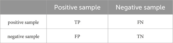
Table 4. Confusion matrix.

Recall represents the ratio of true positive samples found by the model to the total number of positive samples, describing how many positive samples the model can predict from all positive samples. Precision represents the ratio of true positive samples found by the model to the total number of samples predicted as positive by the model, describing how many of the positive samples predicted by the model are truly positive. There is a certain conflict between Recall and Precision, and it is difficult to achieve high values for both. Generally speaking, when precision is high, Recall tends to be low; and when Recall is high, Precision tends to be low (Duan et al., 2020). To improve Recall, it is necessary to predict as many samples as possible as positive, but this increases the probability of misjudgment and reduces precision. To improve Precision, it is necessary to predict samples as positive more cautiously, but this can easily miss some positive samples with less obvious features, reducing Recall. To comprehensively consider Recall and Precision for model evaluation, the following two comprehensive evaluation metrics are introduced: ${\mathrm{F}}_{\mathrm{1}}$ score and ${\mathrm{T}}_{\mathrm{s}\mathrm{s}}$ (true skill statistic) (Bloomfield et al., 2012). The ${\mathrm{F}}_{\mathrm{1}}$ score (Equation 3a) and ${\mathrm{T}}_{\mathrm{s}\mathrm{s}}$ (Equation 3b) are defined as.

${\mathrm{F}}_{\mathrm{1}}=\left(2\times \mathrm{P}\mathrm{r}\mathrm{e}\mathrm{c}\mathrm{i}\mathrm{s}\mathrm{i}\mathrm{o}\mathrm{n}\times \mathrm{R}\mathrm{e}\mathrm{c}\mathrm{a}\mathrm{l}\mathrm{l}\right)/\left(\mathrm{P}\mathrm{r}\mathrm{e}\mathrm{c}\mathrm{i}\mathrm{s}\mathrm{i}\mathrm{o}\mathrm{n}+\mathrm{R}\mathrm{e}\mathrm{c}\mathrm{a}\mathrm{l}\mathrm{l}\right),(\mathrm{3a})$

${\mathrm{T}}_{\mathrm{s}\mathrm{s}}=\mathrm{T}\mathrm{P}/\left(\mathrm{T}\mathrm{P}+\mathrm{F}\mathrm{N}\right)-\mathrm{F}\mathrm{P}/\left(\mathrm{T}\mathrm{N}+\mathrm{F}\mathrm{P}\right),(\mathrm{3b})$

The ${\mathrm{F}}_{\mathrm{1}}$ score is the harmonic mean of Recall and Precision, considering both evaluation metrics comprehensively. ${\mathrm{T}}_{\mathrm{s}\mathrm{s}}$ is obtained by subtracting the ratio of false positives to the total number of negative samples from the Recall, also considering both Recall and Precision. However, in imbalanced classification, the total number of negative samples is often much higher than the number of positive samples, so ${\mathrm{T}}_{\mathrm{s}\mathrm{s}}$ tends to favor Recall.

In this paper, Recall, Precision, ${\mathrm{F}}_{\mathrm{1}}$ score, and ${\mathrm{T}}_{\mathrm{s}\mathrm{s}}$ are used as the main evaluation metrics for models.

Additionally, we select four solar active regions$(\mathrm{A}\mathrm{R}12257,\mathrm{A}\mathrm{R}12468,\mathrm{A}\mathrm{R}12325,\mathrm{A}\mathrm{R}12443)$ to compare their differences in feature importance.

5 Results and discussions

We have selected and processed two types of flare data sets, namely C-class and M-class, separately. Firstly, we input all the features into the BRF, RBC, and NGB model for training and testing. Adjust the hyper-parameter of BRF, RBC, and the threshold probability value of NGB, on the validation set. The final hyper-parameters settings or threshold probability value are obtained by maximizing the ${\mathrm{T}}_{\mathrm{s}\mathrm{s}}$ on the validation set as the tuning target. For BRF, there are two hyper-parameters to be adjusted: the number of decision tree (ntree) and the size of the random feature subset (mtry). The tuning ranges are set as ntree $\in [\mathrm{2,9}]$ with an interval of 1, and mtry $\in [\mathrm{200,1000}]$ with an interval of 200. For RBC, two hyper-parameters are adjusted: the learning rate and the number of boosting iterations (n-boost). The tuning ranges are set as learning rate$\in [0.2,1.2]$ with an interval of 0.2, and $n-boost\in [\mathrm{50,140}]$ with an interval of 10. Figure 2 shows the changes in ${\mathrm{T}}_{\mathrm{s}\mathrm{s}}$ score with respect to different hyper-parameter for the BRF and RBC model on the C and M data set. The highest point corresponds to the optimal combination of hyper-parameters. Therefore, the final hyper-parameters settings obtained are: (1) For BRF on the C data set, ntree$=1000$ and mtry$=2$ (shown in Figure 2A) (2) For BRF on the M data set, ntree$=1000$ and mtry$=6$ (shown in Figure 2B) (3) For RBC on the C data set, learning rate$=0.4$ and n-boost$=100$ (shown in Figure 2C) (4) For RBC on the M data set, learning rate$=0.2$ and n-boost$=50$ (shown in Figure 2D). For NGB, the based learner is set as a decision tree, the scoring rule is logarithmic scoring, and the fitting distribution is a normal distribution. The critical probability value (p) is adjusted within the range of $p\in [0.01,0.6]$ with an interval of 0.01. Figure 3 are line graphs showing the changes in evaluation metrics with respect to the threshold probability value p on the C and M data set, respectively. In Figure 3A, as the threshold probability value p increases, the conditional probability required for predicting a sample label as positive also increases, making the model’s prediction strategy for positive samples more conservative. The corresponding changes in Recall and Precision are that Recall decreases with the increase of p, while Precision increases with the increase of p. This verifies the conflict between recall and precision mentioned earlier. The comprehensive evaluation metrics ${\mathrm{F}}_{\mathrm{1}}$ score and ${\mathrm{T}}_{\mathrm{s}\mathrm{s}}$ both increase first and then decrease with the increase of p. Taking the critical probability value p corresponding to the maximum ${\mathrm{T}}_{\mathrm{s}\mathrm{s}}$, at this time $\mathrm{p}=0.2$. In Figure 3B, Recall decreases with the increase of p, Precision increases with the increase of p, and the comprehensive evaluation metrics ${\mathrm{F}}_{\mathrm{1}}$ score and ${\mathrm{T}}_{\mathrm{s}\mathrm{s}}$ both increase first and then decrease with the increase of p. Due to the more severe imbalance on the M data set, ${\mathrm{T}}_{\mathrm{s}\mathrm{s}}$ only shows an upward and then downward trend within the range of [0,0.1], and decreases with the increase of p when p is greater than 0.1. There are large fluctuations in the ${\mathrm{T}}_{\mathrm{s}\mathrm{s}}$ values at an interval of 0.01. To further refine the value of p, a line graph showing the changes in the four evaluation metrics with respect to the threshold probability value $p$ is plotted within the parameter tuning range of $\mathrm{p}\in [0.001,0.1]$ with an interval of 0.001, as shown in Figure 3C. In Figure 3C, the threshold probability value $p$ corresponding to the maximum ${\mathrm{T}}_{\mathrm{s}\mathrm{s}}$ is chosen, which in this case is $\mathrm{p}=0.034$. Tables 5, 6 represent the evaluation metrics of each model on the C and M data set, respectively. On the C data set, the ${\mathrm{T}}_{\mathrm{s}\mathrm{s}}$ of the three models on the test set all exceeded 0.6 with both the Recall of RBC and NGB exceeding 0.75. While BRF has a Recall of 0.68, it has the highest Precision among the three models, resulting in the highest ${\mathrm{F}}_{\mathrm{1}}$ score. On the M data set, the ${\mathrm{T}}_{\mathrm{s}\mathrm{s}}$ of the three models on the test set all exceeded 0.75. Among them, the Recalls of RBC and NGB both exceeded 0.85, while the Recall of BRF was slightly lower at 0.76. However, BRF had the highest Precision among the three models, resulting in the highest ${\mathrm{F}}_{\mathrm{1}}$ score. The performance of the three models is consistent on both of the C and M data set. To better demonstrate the advantages of these three methods in dealing with imbalanced data sets, we use RF and XGB as two comparison methods. For the prediction results of imbalanced data, the ability to accurately predict the minority positive samples becomes a key criterion for evaluating the performance of a model. Therefore, Recall and ${\mathrm{T}}_{\mathrm{s}\mathrm{s}}$ serve as the primary metrics for assessing such problems. By comparing, Recall and ${\mathrm{T}}_{\mathrm{s}\mathrm{s}}$, BRF, RBC and NGB demonstrate remarkable advantages than RF and XGB.

Figure 2

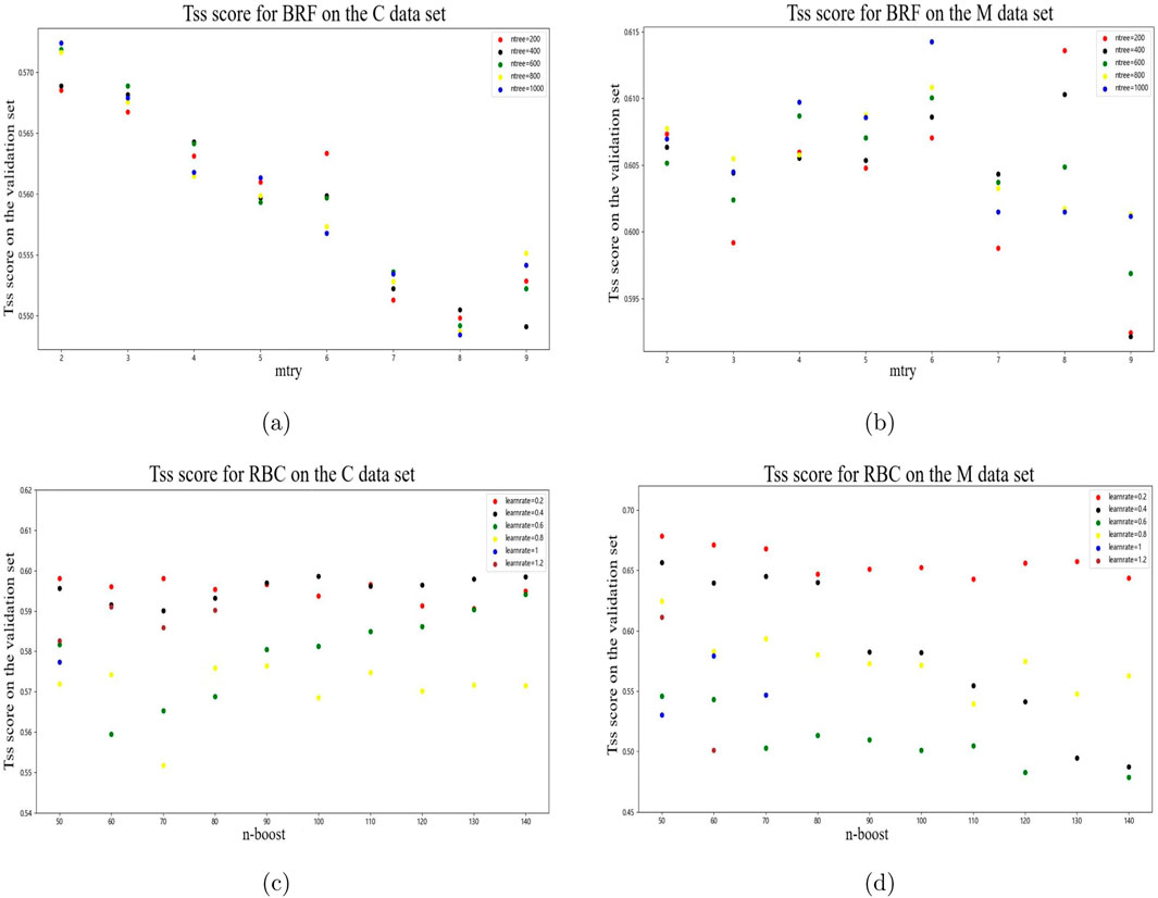
Figure 2. Changes in ${\mathrm{T}}_{\mathrm{s}\mathrm{s}}$ score with respect to different hyper-parameters for the BRF and RBC model on the C and M data set. (A) BRF and C data set (B) BRF and M data set (C) RBC and C data set (D) RBC and M data set.

Figure 3

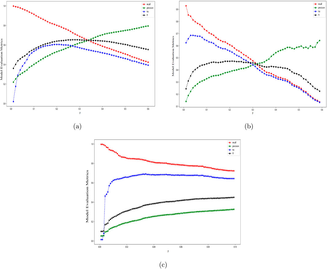
Figure 3. Line graphs showing the changes in evaluation metrics with respect to the threshold probability value p. (A) on C data set (B) graph1 on M data set (C) graph2 on M data set.

Table 5

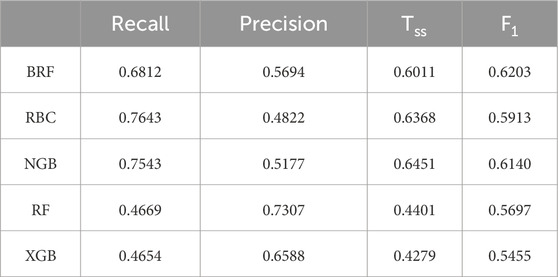
Table 5. Evaluation indicators of each model on the C data set.

Table 6

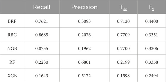
Table 6. Evaluation indicators of each model on the M data set.

The feature importance rankings obtained by the three methods on C data set are shown in Figure 4. Since the parameter distribution fitted in the NGB model is normal distribution with a parameter dimension of 2, the NGB model outputs two rankings of importance scores. Observing these Figures, there is some overlap in the features with high importance scores across various models, but there are also significant differences. Edec and MEANPOT remain in the top ten in four different importance score rankings. TOTUSJH, Cdec, MEANALP, EPSX, and ABSNJZH rank in the top ten in three different importance score rankings. While TOTPOT, USFLUX, TOTBSQ, Xmax1d, and TOTFY rank in the top ten in two different importance score rankings. Additionally, SAVNCPP, Chis, MEANJZD, Bhis, Chis1d, TOTUSJZ, and EPSY only rank in the top ten in one of the importance scores.

Figure 4

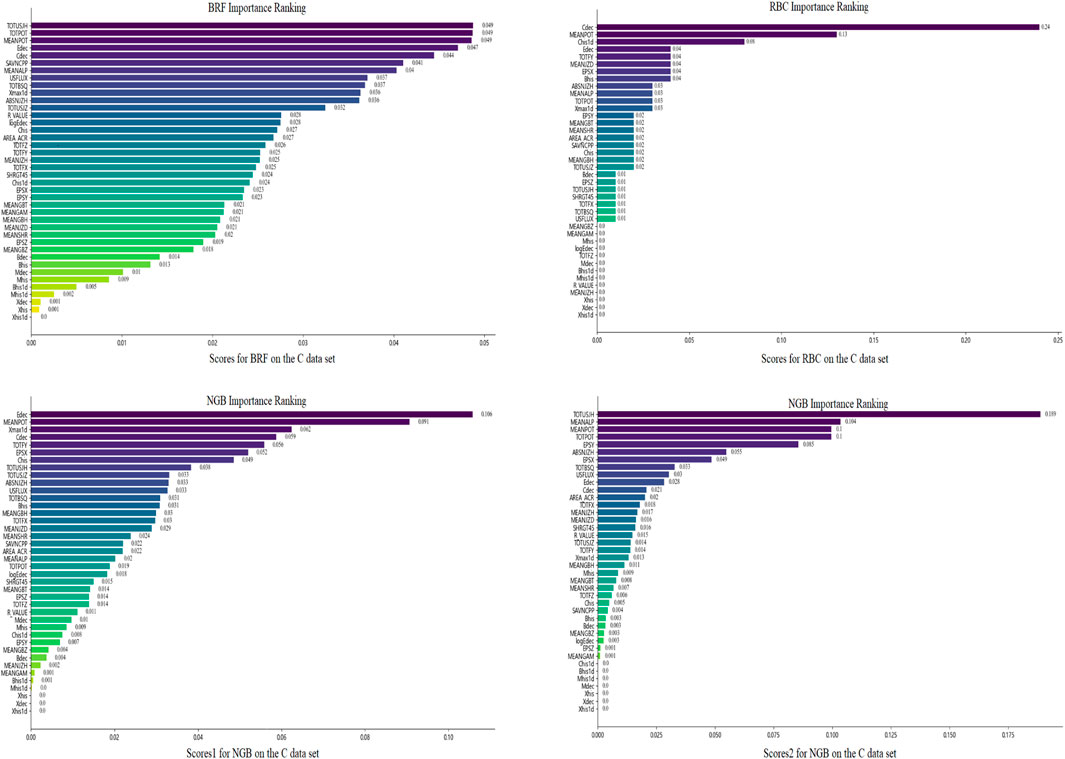
Figure 4. Feature importance ranking obtained by the three methods (BRF, RBC, and NGB) on the C data set.

The feature importance rankings obtained by the three methods on M data set are shown in Figure 5. In these sub-figures, we can see that there is some overlap in the features with high importance scores across various models, but there are also significant differences. Edec, MEANPOT, and TOTUSJH consistently rank in the top ten in four different importance score rankings. TOTUSJZ ranks in the top ten in three different importance score rankings, while Xmax1d, Cdec, ABSNJZH, Chis1d, EPSX, MEANGBH, logEdec, and TOTFX rank in the top ten in two different importance score rankings. Additionally, TOTPOT, TOTBSQ, USFLUX, Bhis, AREA-ACR, MEANALP, Xdec, SAVNCPP, and SHRGT only rank in the top ten in one of the importance scores.After obtaining the importance rankings score for each feature within each model, we averaged these scores across the three models to determine the comprehensive importance ranking. The results for the C and M data sets are presented in Table 7 and Table 8, respectively. Ran et al. (2022) studied the most relevant to flares with 16 SHARP parameters by calculating correlation coefficients and variable importance scores, and they identified eight parameters (TOTPOT, MEANPOT, USFLUX, MEANGAM, MEANJZH, MEANGBH, MEANALP, MEANSHR) most relevant to flares. All of these features are physical parameters describing magnetic field characteristics. In fact, TOTPOT and MEANPOT represent the same characteristic, while the other six parameters are all related to the distortion and deformation of the magnetic field. We have analyzed more characteristics, including 40 parameters, not only parameters related to the magnetic field, but also additional historical information of flare occurrences and exponential time decay values. According to Tables 7, 8, MEANPOT, Edec, and TOTUSJH have high importance scores on the two data sets. They are three quantities that have the most significant relationship with solar flares, which include free energy, twist degree, and the historical information of flare occurrences, respectively. Moreover, there is a high overlap between the top ten features in terms of importance on the two data sets, with seven features appearing in the top ten of both lists: MEANPOT, Cdec, Edec, TOTUSJH, ABSNJZH, Xmax1d, and EPSX. Among them, Cdec, Edec, and Xmax1d are all features related to historical flare data, indicating that flare history data contributes significantly to flare prediction. Furthermore, compared to simple counting of historical data, exponential time decay values are more valuable in prediction. Meanwhile, MEANPOT, TOTUSJH, ABSNJZH, and EPSX are physical parameters that describe the overall magnetic field situation and also have high importance scores in flare prediction. This aligns with reality because solar flare eruptions involve a significant process of storing and releasing free energy. The frequency and temporal decay characteristics of flare eruptions in an active region represent the vitality of that region. Active regions that store a large amount of free energy and experience frequent eruptions with low decay rates are more likely to generate flares.

Using the comprehensive ranking of feature importance obtained in Section 4, feature selection is performed for the three prediction models. Starting from a model trained with at least two features, features are added in descending order of importance. Observe the changes in the evaluation index values of the BRF, RBC, and NGB models trained with different numbers of features on the C data set, as shown in the following figure: In Figure 6A, as the number of features increases, the Recall of the BRF model on the validation set generally decreases, while the Precision generally increases. When the number of features is greater than or equal to 15, the Recall and Precision are basically stable, and the ${\mathrm{F}}_{\mathrm{1}}$ score and ${\mathrm{T}}_{\mathrm{s}\mathrm{s}}$ also tend to stabilize. In Figure 6B, when the number of features is less than 20, four evaluation indicators of RBC fluctuate violently with the change of feature numbers, and the performance is very unstable. When the number of features is greater than or equal to 20, the Recall, Precision, ${\mathrm{F}}_{\mathrm{1}}$ score, and ${\mathrm{T}}_{\mathrm{s}\mathrm{s}}$ all tend to stabilize. In Figure 6C, the evaluation metrics of NGB change little with the increase of feature numbers. The Recall shows a slow growth trend, while the Precision shows a slow decreasing trend. There is only a large fluctuation when the number of features increases from 2 to 3. And the Recall tends to be stable when the number of features is greater than or equal to 22, and at this time, the ${\mathrm{F}}_{\mathrm{1}}$ score and ${\mathrm{T}}_{\mathrm{s}\mathrm{s}}$ tend to be stable. Based on the prediction performance of the above three models under different feature quantities, the number of BRF features is selected as 15, the number of RBC features as 20, and the number of NGB features as 23.

Figure 5

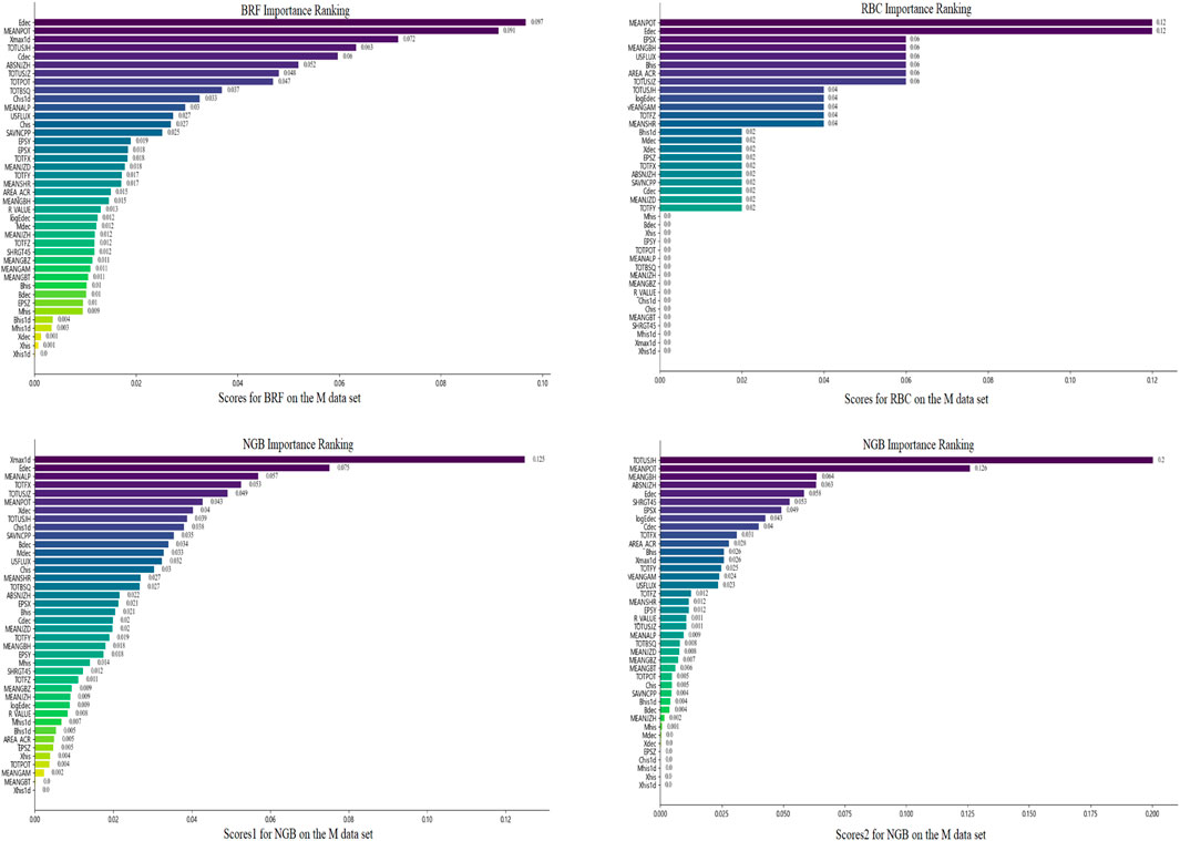
Figure 5. Feature importance ranking obtained by the three methods (BRF, RBC, and NGB) on the M data set.

Figure 6

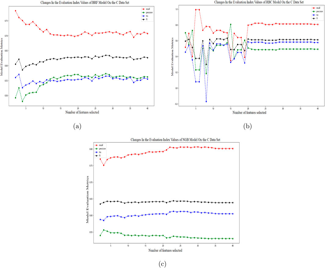
Figure 6. Line graphs of four evaluation metrics changing with the number of features by the three methods [(A) BRF (B) RBC (C) NGB] on the C data set.

Table 7

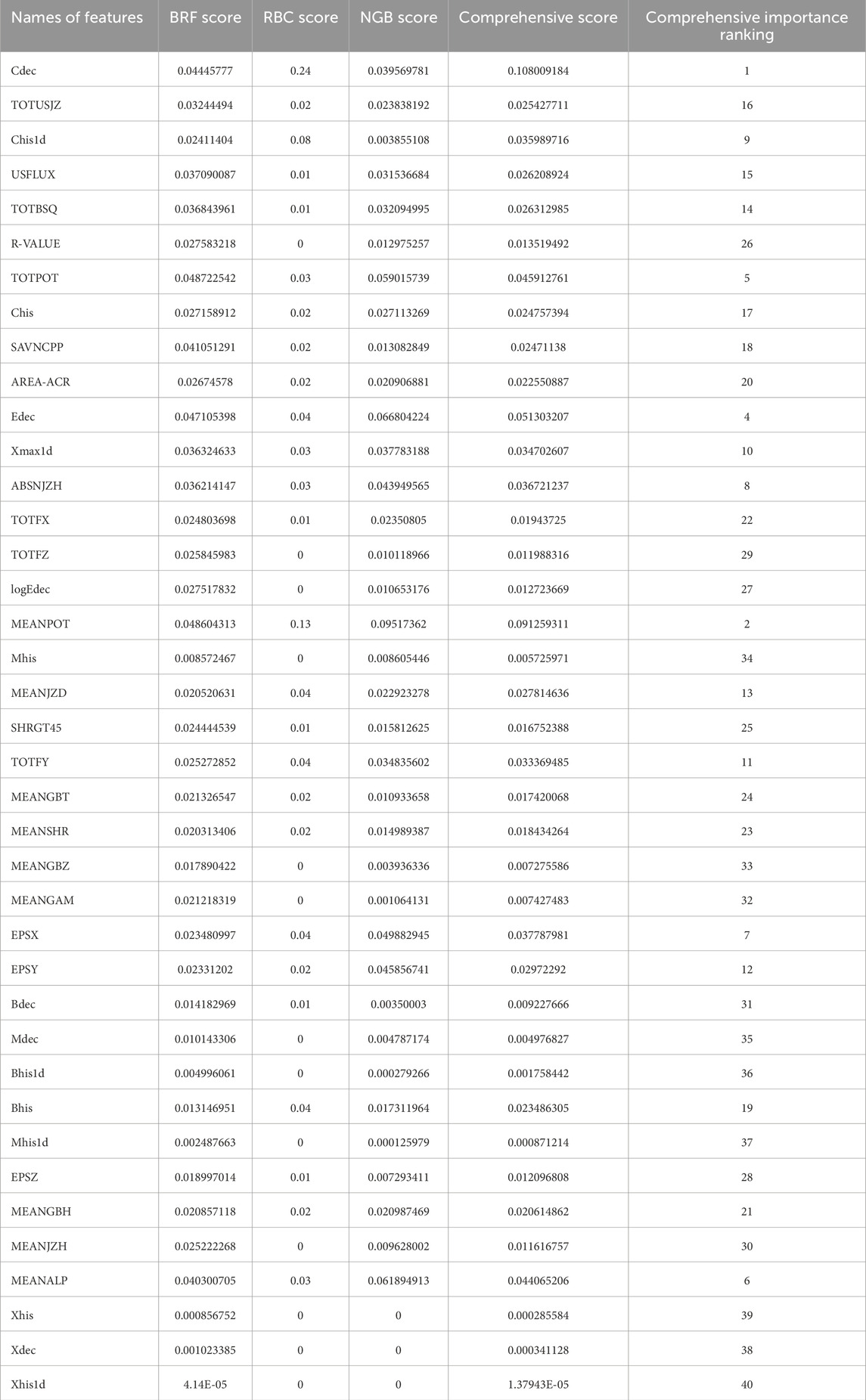
Table 7. Comprehensive importance ranking on C data set.

Table 8

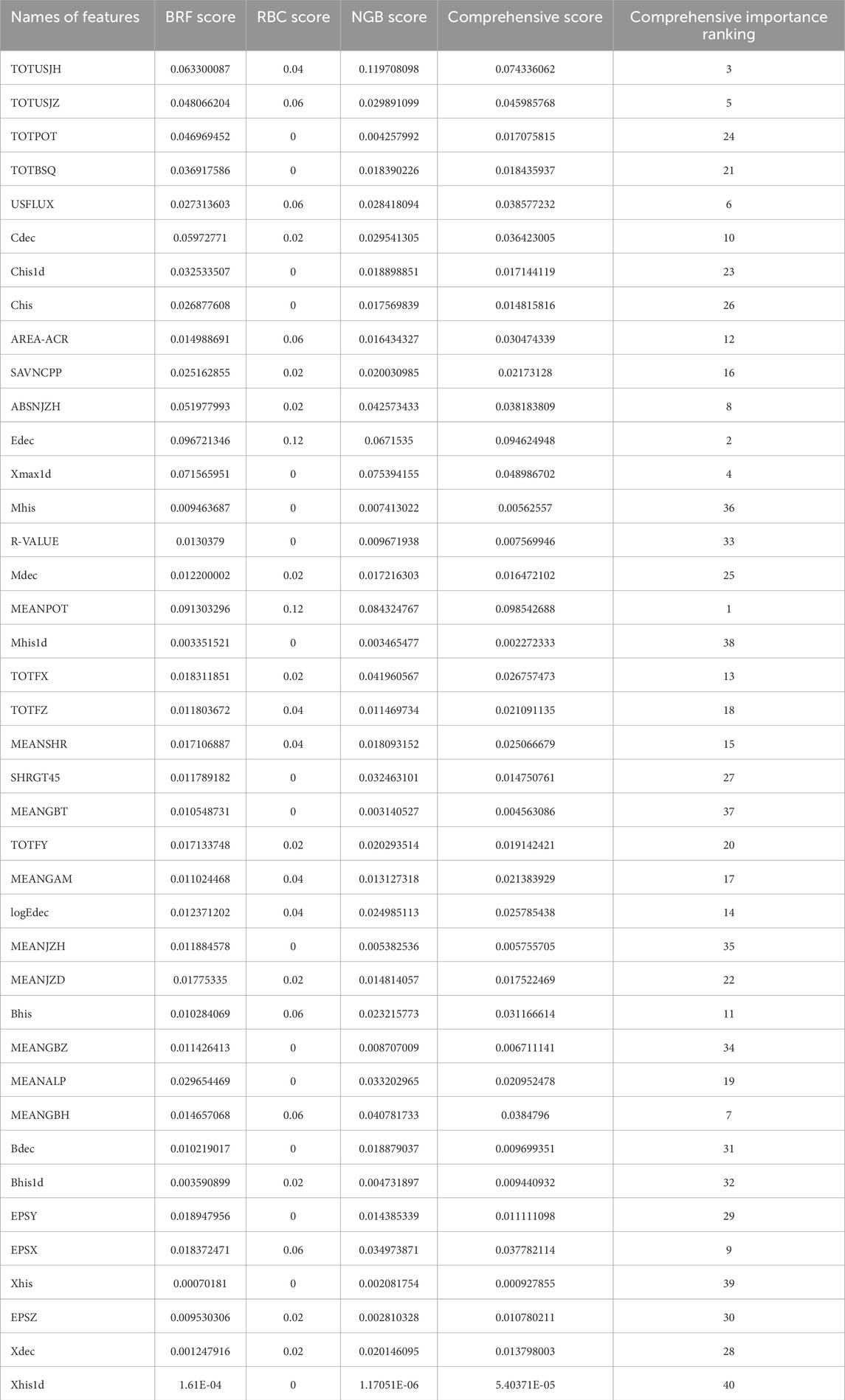
Table 8. Comprehensive importance ranking on M data set.

The evaluation metrics of the three models on the training set after feature selection are as follows: Comparing the evaluation indicators of the three models in Table 5 and Table 9, after feature selection, the prediction effects of BRF, RBC, and NGB models are basically consistent with those before feature selection. The difference in ${\mathrm{T}}_{\mathrm{s}\mathrm{s}}$ scores is less than 0.02, while the ${\mathrm{F}}_{\mathrm{1}}$ scores of BRF and RBC are slightly lower than those before feature selection, and the ${\mathrm{F}}_{\mathrm{1}}$ score of NGB is slightly higher. After feature selection, the biggest loss of prediction performance is BRF. Observing the changes in various evaluation metrics of the BRF, RBC, and NGB models trained with different numbers of features on the M validation set, as shown in Figure 7: Based on the prediction performance of the above three models with varying feature quantities, we selected 12 features for BRF, 26 for RBC, and 18 for NGB. Comparing Tables 6 and 10, after feature selection, the prediction effects of the three models, BRF, RBC, and NGB, all showed slight improvements. Among them, the ${\mathrm{T}}_{\mathrm{s}\mathrm{s}}$ scores of RBC and NGB increased by less than 0.01, while the ${\mathrm{T}}_{\mathrm{s}\mathrm{s}}$ score of BRF improved by 0.044. Feature selection enhanced both the Recall and Precision of the BRF model. Furthermore, we analyzed the textual feature parameters of four active regions $(\mathrm{A}\mathrm{R}12257,\mathrm{A}\mathrm{R}12468,\mathrm{A}\mathrm{R}12325,\mathrm{A}\mathrm{R}12443)$ using three ensemble machine learning models (RF, XGB, and NGB). Figures 8–11 present the feature importance rankings obtained by these three models. By summing the scores from the four results, we derived the final feature importance ranking, as shown in Table 11. From these results, we observe that the temporal decay parameter for flare history (Cdec) and physical parameters reflecting the overall magnetic field conditions, such as TOTUSJH, TOTBSQ, SAVNCPP, and MEANALP, consistently exhibit high feature importance across different active regions. Conversely, features related to coordinate directions and positions, including EPSZ, EPSY, and EPSX, show significant variations in their importance rankings across different ARs. This indicates that the importance of parameters related to location may vary in different activity zones. When analyzing and predicting solar flares, geographic location information is also a factor that should be considered. Firstly, the probability of flare occurrence varies with different latitudes. As the latitude of the active region reflects the activity of the current solar cycle, and the size of active regions varies at different locations, according to Murakozy (2024), larger active regions may have a higher number of interacting sunspots and a smaller distance between the positive and negative poles of newly emerged sunspots, leading to differences in activity among different active regions. Secondly, the surrounding environment of an active region can also affect its eruptive activities. For example, medium and low latitudes are easily influenced by some coronal streams, while the magnetic fields in medium and high latitude active regions are relatively weak. Additionally, there may be influences from generator effects such as meridional circulations, all of which will be reflected in the location of the active regions. If the geographical location factors of different active regions are ignored, some information will be lost.

Table 9

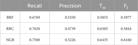
Table 9. Evaluation metrics of each model on the C data set after feature selection.

Figure 7

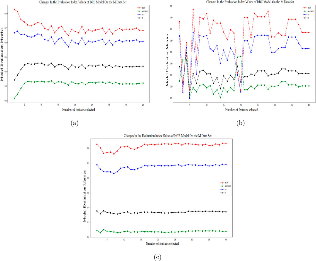
Figure 7. Line graphs of four evaluation metrics changing with the number of features by the three methods [(A) BRF (B) RBC (C) NGB] on the M data set.

Table 10

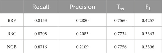
Table 10. Evaluation metrics of each model on the M data set after feature selection.

Figure 8

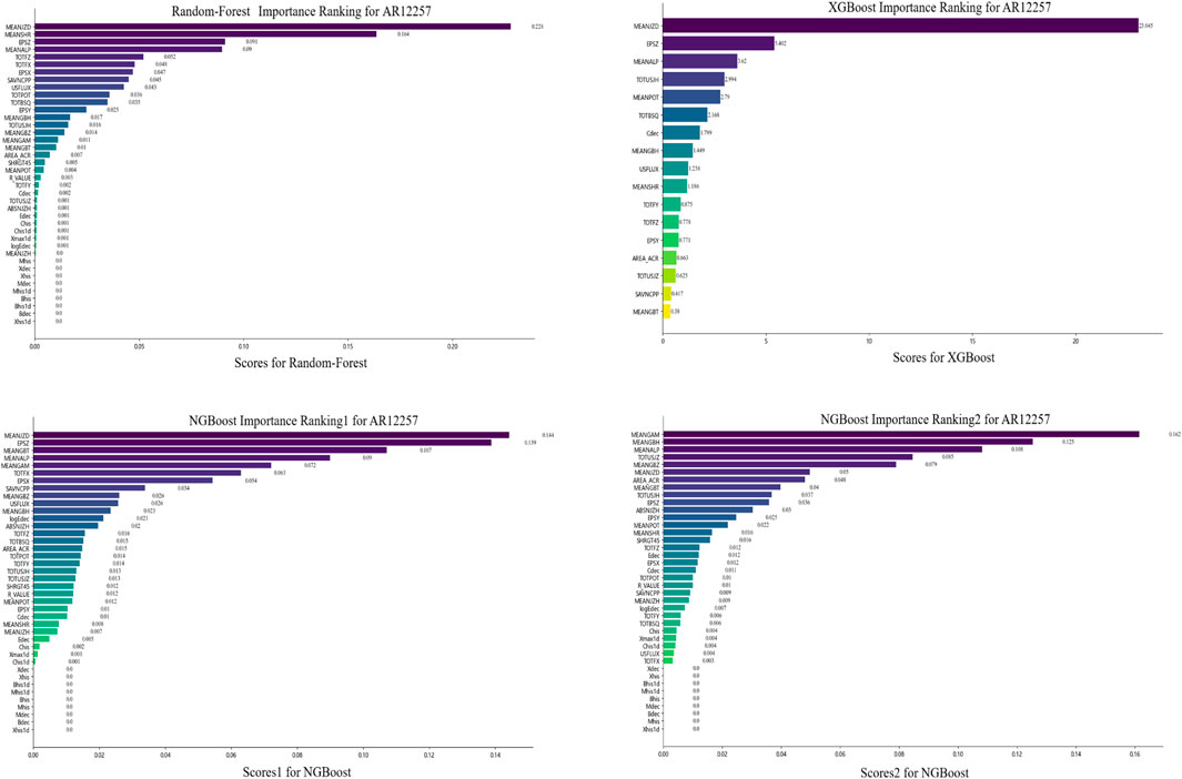
Figure 8. Feature importance rankings with three ensemble machine learning models (RF, XGB, and NGB) for AR12257.

Figure 9

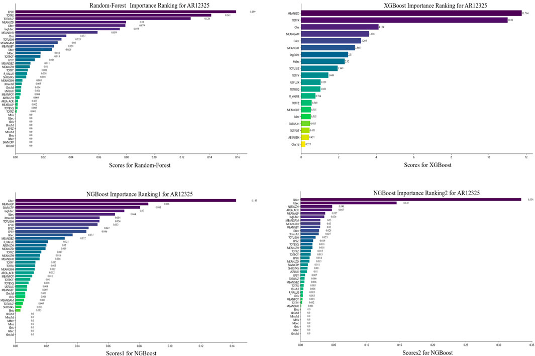
Figure 9. Feature importance rankings with three ensemble machine learning models (RF, XGB, and NGB) for AR12468.

Figure 10

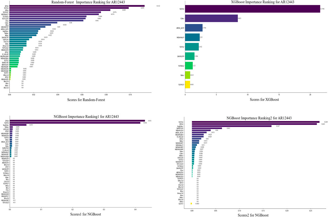
Figure 10. Feature importance rankings with three ensemble machine learning models (RF, XGB, and NGB) for AR12325.

Figure 11

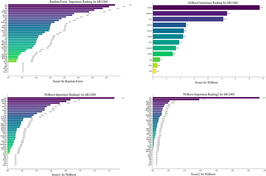
Figure 11. Feature importance rankings with three ensemble machine learning models (RF, XGB, and NGB) for AR12443.

Table 11

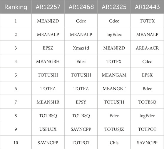
Table 11. Top 10 features ranked by importance in different ARs.

6 Conclusion

In this study, we focus on solar flare prediction and the analysis of the importance of predictive features. It encompasses the collection and preprocessing of flare-related data, the training of classification models with data and algorithms, the hyper-parameter tuning of the classification models, the derivation of feature importance scores and rankings, the feature selection of the prediction model based on feature importance results, and the evaluation of the model’s predictive performance on a test set. After collecting and processing the data, we employ ensemble learning algorithms and imbalanced sampling techniques to train an initial prediction model. Through this model, we obtain variable importance scores and synthesize scores from different methods to derive a comprehensive ranking of the importance of each variable. By comparing the importance scores of variables from different solar active regions, we identify their differences and commonalities, which serve as the basis for feature selection. We utilize ensemble learning methods to construct classification models and adjust hyper-parameters to improve classification performance. Finally, we compare the classification results of different methods, as well as the results before and after feature selection, to explore avenues for improving the prediction of solar flares. We use three ensemble learning algorithms to perform binary classification predictions for flares $\ge$ C- and M-class. By employing sampling techniques and probability distribution predictions, the predictive performance on imbalanced flare data sets is improved. The main research conclusions are as follows:

(1) Three ensemble learning algorithms suitable for imbalanced classification predictions, namely BRF, RBC, and NGB, are used to construct prediction models. For the prediction of flares $\ge$ C- and M-class, the best-performing model achieved a Recall of $\sim 0.76$, $\sim 0.88$ and a ${\mathrm{T}}_{\mathrm{s}\mathrm{s}}$ score of $\sim 0.65$, $\sim 0.78$ on the test set, respectively. Comparing the performance of the three models across various evaluation metrics, BRF is more conservative in predicting positive samples, with a lower Recall rate than the other two models, but correspondingly, it has a higher Precision rate. RBC and NGB have higher Recall rates and slightly higher ${\mathrm{T}}_{\mathrm{s}\mathrm{s}}$ scores than BRF. Since NGB performs probability distribution predictions, the probability threshold can be adjusted according to actual needs to balance between Recall and Precision.

(2) Feature importance scores are obtained through the three ensemble learning models directly obtained through the model without the need for additional feature analysis tools. The results from different models are integrated in the form of rankings. Using this ranking for feature selection in the prediction model, only about half of the features with strong importance are needed to achieve similar or even better prediction performance compared to using all 40 features.

(3) Comparing the feature importance rankings of the flare prediction models for $\ge$ C- and M-class, a high degree of overlap is found. Our results demonstrate the magnetic field, historical information of flare occurrences and exponential time decay values have the most significant relationship with solar flares. This also means that frequency and temporal decay characteristics of flare eruptions in an active region represent the vitality of that region. Active regions that store a large amount of free energy and experience frequent eruptions with low decay rates are more likely to generate flares. By analyzing the feature parameters of four active regions, we find that the geographical information of the flare occurrence is an important factor for flare prediction.

In this research, there are still some limitations. The number of ARs selected for studying the differences in feature importance across different ARs is relatively small, which cannot reflect the overall pattern of feature importance for global ARs. In future work, we will select data from more active regions for analysis based on their distribution characteristics. In addition, the hyper-parameters of the model can be further adjusted and optimized to achieve much better prediction results.

Data availability statement

The original contributions presented in the study are included in the article/supplementary material, further inquiries can be directed to the corresponding author.

Author contributions

YY: Writing–original draft, Writing–review and editing.

Funding

The author(s) declare that financial support was received for the research, authorship, and/or publication of this article. This research was supported by the National Key Technologies Research and Development Program of the Ministry of Science and Technology of China (2021YFA1600504) and the National Natural Science Foundation of China (42204155) and Natural Science Foundation of Jiangsu, China (BK20210168).

Acknowledgments

All the data and the source codes used in this paper are available on the website https://github.com/Yangyun-Group/CME for the researchers who have interest in applying them to manipulate their own data.

Conflict of interest

The author declares that the research was conducted in the absence of any commercial or financial relationships that could be construed as a potential conflict of interest.

Generative AI statement

The author(s) declare that no Generative AI was used in the creation of this manuscript.

Publisher’s note

All claims expressed in this article are solely those of the authors and do not necessarily represent those of their affiliated organizations, or those of the publisher, the editors and the reviewers. Any product that may be evaluated in this article, or claim that may be made by its manufacturer, is not guaranteed or endorsed by the publisher.

References

Baker, D., Daly, E., Daglis, I., Kappenman, J., and Panasyuk, M. (2004). Effects of space weather on technology infrastructure. Space Weather Int. J. Res. Appl. 2. doi:10.1029/2003SW000044

CrossRef Full Text | Google Scholar

Berk, R. A. (2016). Classification and regression trees (CART). Cham: Springer International Publishing, 129–186. doi:10.1007/978-3-319-44048-4_3

CrossRef Full Text | Google Scholar

Bloomfield, D. S., Higgins, P. A., McAteer, R. T. J., and Gallagher, P. T. (2012). Astrophysical J. Lett. 747, L41. doi:10.1088/2041-8205/747/2/L41

CrossRef Full Text | Google Scholar

Bobra, M. G., and Couvidat, S. (2014). Solar flare prediction usingsdo/hmi vector magnetic field data with a machine-learning algorithm. Astrophysical J. 798, 135. doi:10.1088/0004-637X/798/2/135

CrossRef Full Text | Google Scholar

Boucheron, L. E., Al-Ghraibah, A., and McAteer, R. T. J. (2015). Astrophysical J. 812, 51. doi:10.1088/0004-637X/812/1/51

CrossRef Full Text | Google Scholar

Breiman, L. (2001). Mach. Learn. 45, 5–32. doi:10.1023/a:1010933404324

CrossRef Full Text | Google Scholar

Chen, C., and Breiman, L. (2004). Berkeley: University of California.

Google Scholar

Chen, P. (2011). Coronal mass ejections: models and their observational basis. Sol. Phys. 8. doi:10.12942/lrsp-2011-1

CrossRef Full Text | Google Scholar

Chen, Y., Manchester, W. B., Hero, A. O., Toth, G., DuFumier, B., Zhou, T., et al. (2019). Identifying solar flare precursors using time series of SDO/HMI images and SHARP parameters. Space weather. 17, 1404–1426. doi:10.1029/2019SW002214

CrossRef Full Text | Google Scholar

Deshmukh, V., Baskar, S., Berger, T. E., Bradley, E., and Meiss, J. D. (2023). Comparing feature sets and machine-learning models for prediction of solar flares: topology, physics, and model complexity. Astronomy Astrophysical 674, A159. doi:10.1051/0004-6361/202245742

CrossRef Full Text | Google Scholar

Duan, T., Avati, A., Ding, D. Y., Thai, K. K., Basu, S., Ng, A. Y., et al. (2020). “International conference on machine learning”, in Proceedings of the 37th International Conference on Machine Learning. Editor H. Daumé, III, and S. Aarti (PMLR) 119, 2690–2700. Available at: https://proceedings.mlr.press/v119/duan20a.html.

Google Scholar

Feng, X. (2020). Magnetohydrodynamic modeling of the solar corona and heliosphere. Singapore: Springer, 1–763. doi:10.1007/978-981-13-9081-4

CrossRef Full Text | Google Scholar

Fisher, G., Bercik, D., Welsch, B., and Hudson, H. S. (2012). Global forces in eruptive solar flares: the lorentz force acting on the solar atmosphere and the solar interior. Sol. Phys. 277, 59–76. doi:10.1007/s11207-011-9907-2

CrossRef Full Text | Google Scholar

Gallagher, H., Jack, A., Roepstorff, A., and Frith, C. (2002). Imaging the intentional stance in a competitive game. NeuroImage 16, 814–821. doi:10.1006/nimg.2002.1117

PubMed Abstract | CrossRef Full Text | Google Scholar

He, H., and Garcia, E. A. (2009). Learning from imbalanced data. IEEE Trans. Knowl. Data Eng. 21, 1263–1284. doi:10.1109/TKDE.2008.239

CrossRef Full Text | Google Scholar

He, X. (2021). Phdthesis, university of Chinese Academy of Sciences national space science center. China: Chinese Academy of Sciences. doi:10.27562/d.cnki.gkyyz.2021.000023

CrossRef Full Text | Google Scholar

Huang, X., Wang, H., Xu, L., Liu, J., Li, R., and Dai, X. (2018). Deep learning based solar flare forecasting model. I. Results for line-of-sight magnetograms. Astrophysical J. 856, 7. doi:10.3847/1538-4357/aaae00

CrossRef Full Text | Google Scholar

Jing, J., Yurchyshyn, V., Yang, G., Xu, Y., and Wang, H. (2004). On the relation between filament eruptions, flares, and coronal mass ejections. Astrophysical J. 614, 1054–1062. doi:10.1086/423781

CrossRef Full Text | Google Scholar

Jonas, E., Bobra, M., Shankar, V., Todd Hoeksema, J., and Recht, B. (2018). Flare prediction using photospheric and coronal image data. Sol. Phys. 293, 48. doi:10.1007/s11207-018-1258-9

CrossRef Full Text | Google Scholar

Li, R., Wang, H.-N., He, H., Cui, Y.-M., and Du, Z. L. (2007). Support vector machine combined with K-nearest neighbors for solar flare forecasting. ChJA& 7, 441–447. doi:10.1088/1009-9271/7/3/15

CrossRef Full Text | Google Scholar

Liu, C., Deng, N., Wang, J. T. L., and Wang, H. (2017). Predicting solar flares using SDO/HMI vector magnetic data products and the random forest algorithm. Astrophysical J. 843, 104. doi:10.3847/1538-4357/aa789b

CrossRef Full Text | Google Scholar

Liu, H., Liu, C., Wang, J. T. L., and Wang, H. (2019). Predicting solar flares using a Long short-term memory network. Astrophysical J. 877, 121. doi:10.3847/1538-4357/ab1b3c

CrossRef Full Text | Google Scholar

Mason, J. P., and Hoeksema, J. T. (2010). ApJ 723, 634–640. doi:10.1088/0004-637X/723/1/634

CrossRef Full Text | Google Scholar

Murakozy, J. (2024). Variation in the polarity separation of sunspot groups throughout their evolution. Astronomy Astrophysics 690, A257. doi:10.1051/0004-6361/202450194

CrossRef Full Text | Google Scholar

Nishizuka, N., Sugiura, K., Kubo, Y., Den, M., Watari, S., and Ishii, M. (2017). Solar flare prediction model with three machine-learning algorithms using ultraviolet brightening and vector magnetograms. Astrophysical J. 835, 156. doi:10.3847/1538-4357/835/2/156

CrossRef Full Text | Google Scholar

Priest, E. R., and Forbes, T. G. (2002). The magnetic nature of solar flares. A& Rv 10, 313–377. doi:10.1007/s001590100013

CrossRef Full Text | Google Scholar

Ran, H., Liu, Y. D., Guo, Y., and Wang, R. (2022). Relationship between successive flares in the same active region and SHARP parameters. Astrophysical J. 937, 43. doi:10.3847/1538-4357/ac80fa

CrossRef Full Text | Google Scholar

Schou, J., Scherrer, P., Bush, R., Wachter, R., Couvidat, S., Rabello-Soares, M. C., et al. (2012). Design and ground calibration of the helioseismic and magnetic imager (HMI) instrument on the solar dynamics observatory (SDO). Sol. Phys. 275, 229–259. doi:10.1007/s11207-011-9842-2

CrossRef Full Text | Google Scholar

Seiffert, C., Khoshgoftaar, T. M., Hulse, J. V., and Napolitano, A. (2010). IEEE Trans. Syst. Man, Cybern. - Part A Syst. Humans 40, 185. doi:10.1109/TSMCA.2009.2029559

CrossRef Full Text | Google Scholar

Sharma, N. (2017). XGBoost. The extreme gradient boosting for mining applications. Comput. Sci., 1–56. doi:10.1029/GM098p0077

CrossRef Full Text | Google Scholar

Shibata, K., and Magara, T. (2011). Solar flares: magnetohydrodynamic processes. Living Rev. Sol. Phys. 8. doi:10.12942/lrsp-2011-6

CrossRef Full Text | Google Scholar

Sinha, S., Gupta, O., Singh, V., Lekshmi, B., Nandy, D., Mitra, D., et al. (2022). A comparative analysis of machine-learning models for solar flare forecasting: identifying high-performing active region flare indicators. Astrophysical J. 935, 45. doi:10.3847/1538-4357/ac7955

CrossRef Full Text | Google Scholar

Song, H., Tan, C., Jing, J., Wang, H., Yurchyshyn, V., and Abramenko, V. (2009). Statistical assessment of photospheric magnetic features in imminent solar flare predictions. Sol. Phys. 254, 101–125. doi:10.1007/s11207-008-9288-3

CrossRef Full Text | Google Scholar

Wang, J., Luo, B., Liu, S., and Zhang, Y. (2023). A strong-flare prediction model developed using a machine-learning algorithm based on the video data sets of the solar magnetic field of active regions. Astrophysical J. Suppl. Ser. 269, 54. doi:10.3847/1538-4365/ad036d

CrossRef Full Text | Google Scholar

Wang, X., Chen, Y., Toth, G., Manchester, W. B., Gombosi, T. I., Hero, A. O., et al. (2020). Predicting solar flares with machine learning: investigating solar cycle dependence. Astrophysical J. 895, 3. doi:10.3847/1538-4357/ab89ac

CrossRef Full Text | Google Scholar

Webb, D. F., and Howard, T. A. (2012). Coronal mass ejections: observations. Living Rev. Sol. Phys. 9, 3. doi:10.12942/lrsp-2012-3

CrossRef Full Text | Google Scholar

Yan, X.-L., Qu, Z.-Q., and Kong, D.-F. (2011). Relationship between eruptions of active-region filaments and associated flares and coronal mass ejections: active-region filaments, flares and CMEs. Mon. Notices R. Astronomical Soc. 414, 2803–2811. doi:10.1111/j.1365-2966.2011.18336.x

CrossRef Full Text | Google Scholar

Yang, Y., Liu, J. J., Feng, X. S., Chen, P. F., and Zhang, B. (2023). Prediction of the transit time of coronal mass ejections with an ensemble machine-learning method. Astrophysical J. Suppl. Ser. 268, 69. doi:10.3847/1538-4365/acf218

CrossRef Full Text | Google Scholar