Variability of Earth’s ionospheric outflow in response to the dynamic terrestrial exosphere

Abstract

The most abundant neutral constituent in the exospheric region (i.e., beyond 500 km altitude) is the atomic hydrogen (H); however, its density distributions predicted by physics-based models have been challenged by satellite-based observations of its far ultraviolet emissions. This discrepancy may impact magnetospheric ions’ densities and velocities since numerous chemistry and ion-neutral coupling interactions rely sensitively on the underlying neutral hydrogen population. The Polar Wind Outflow Model a first-principled model for relevant ion species in the high-latitude ionosphere, is employed to investigate the role of neutral H on the ionospheric outflow. Specifically, variability in the outflow of ionospheric , , , and as a response to systematic enhancement and depletion of H number densities were simulated. The altitude-dependent ion density and energy partition profiles vary with neutral H density, solar activities, and ion species. These findings suggest that the exosphere plays a crucial role in controlling the production and loss of ions through ionospheric chemistry, as well as the energy contributions by altering ion-neutral-electron collisions and the ambipolar electric field to the high-latitude ionospheric outflow. As a result, the escape rates of the ionospheric outflow are directly associated with exospheric distributions. This work potentially helps understand the dominant mechanisms of atmospheric escape, particularly during a hydrogen-rich early Earth’s and exoplanet’s atmosphere, which is known to play a significant role in understanding the evolution of Earth’s atmosphere.

1 Introduction

The terrestrial exosphere is the outermost layer of the atmosphere that extends from the exobase, located at 500 km, to several tens of Earth radii (1 = 6,371 km) (Baliukin et al., 2019). The exosphere predominantly comprises atomic hydrogen (H), which resonantly scatters solar Lyman-Alpha photons (Ly- at 121.6 nm), producing a planetary glow effect known as the geocorona. This emission, acquired by several space-based optical instruments (i.e., TWINS/LAD (McComas et al., 2009), PROCYON/LAICA (Kameda et al., 2017), TIMED/GUVI), has been used together with parametric and tomographic inversion techniques to retrieve 1-D/3-D H density distributions (Waldrop and Paxton, 2013; Joshi et al., 2019; Cucho-Padin and Waldrop, 2018; Cucho-Padin et al., 2022). Knowledge of the global/regional spatial distribution and the temporal evolution of H density is crucial for understanding (a) the physical mechanisms involved in the permanent escape of atomic H to space and (b) the role of this neutral population in determining magnetospheric plasma dynamics. It is noteworthy that the terrestrial exosphere is a dynamic system whose density distribution is directly affected by the thermospheric temperature, displaying significant variability from solar minimum to solar maximum (Zoennchen et al., 2015) as well as rapid variations during storm-time conditions Cucho-Padin and Waldrop (2019).

Due to the vast extension of the exosphere, H atoms may interact with ions from different regions and energy ranges in the magnetosphere-ionosphere system (i.e., plasmasphere, ring current, plasma sheet, ionospheric outflow, and solar wind ions). The ion-neutral coupling occurs via charge exchange interactions in which a hot ion picks up the electron of a cold H atom to become an energetic neutral atom (ENA) that has sufficient energy to escape out the planet since it is not affected by electric or magnetic fields, or return to the thermosphere and act as an additional source of neutral energization. Through charge exchange interactions, the exosphere significantly contributes to the plasmaspheric refilling and ion ring current decay, especially during high geomagnetic activity (Krall et al., 2018; Cucho-Padin et al., 2020a,b).

Current physics- and data-based models of H-density distributions exhibit significant disagreement in both number density () and global/regional spatial structure (Krall et al., 2018). For example, values retrieved by the empirical Mass Spectrometer Incoherent Scatter (NRLMSIS-00, referred to as MSIS in this paper) model (Picone et al., 2002), widely used by the aeronomy and magnetospheric community, have been challenged by data-based estimations derived from radiance data. Waldrop and Paxton (2013) used Ly- data acquired by the Global UltraViolet Imager (GUVI) on board NASA’s Thermosphere Ionosphere Mesosphere Energetics and Dynamics (TIMED) spacecraft along with a parametric technique to retrieve exobase density ( km altitude) during the period 2002 to 2007. This study shows that exobase values obtained from MSIS are 42%–74% larger than those derived from GUVI data at solar maximum and 36%–67% larger during solar minimum. Furthermore, from GUVI data are smaller than from Monte Carlo simulations of Hodges (1994) by an order of magnitude below 1,000 km altitude. In addition, Nossal et al. (2012) conducted a comparison study of column-integrated intensities of Balmer-Alpha emissions (H- at 656 nm) between those acquired by the Wisconsin H-alpha Mapper (WHAM) Fabry-Perot and those derived from MSIS with the exosphere extension proposed by Bishop (1991). As a result, H- intensities derived from the empirical model are 33% smaller than those measured by WHAM. These discrepancies possibly occur due to the limited physical assumptions included in MSIS. While this model considers a thermalized atmosphere (i.e., neutral-neutral collisions in the thermosphere determine the energy partition), other sources of energization, such as charge exchange between H atoms and plasmaspheric ions beyond the exobase, may also occur Qin and Waldrop (2016).

The plasma transport from the ionosphere to the magnetosphere is known as “ionospheric outflow” or “ion outflow.” In the low- and mid-latitude ionosphere, the magnetic field lines connect the two conjugate hemispheres and have direct access to the plasmasphere and ring current, while in the high-latitude ionosphere, the magnetic field lines are open and connect to outer space and the IMF. Based on the source and their destinations in the magnetosphere, the ionospheric outflows are often categorized into low-latitude and high-latitude ionospheric outflows. A previous study unveiled that abundances of sourced from the low-latitude ionospheric outflow are sensitive to the H density distribution and alter the dynamics of the ring current and plasmasphere, especially after geomagnetic storms (Krall et al., 2018). This paper, on the other hand, focuses on the effect of H density on the high-latitude ionospheric outflow, also known as “polar wind.” Since the high-latitude ionospheric outflow can directly interact with the solar wind plasma and IMF, it is exposed to additional suprathermal escape mechanisms, such as Suprathermal Electron (SE) impact (Axford, 1968; Glocer et al., 2012; Glocer et al., 2017) and Wave-Particle Interaction (WPI) (Chang et al., 1986; André et al., 1998; Varney et al., 2016; Glocer and Daldorff, 2022). Therefore, the high-latitude ionospheric outflow is one of the main pathways of heavy ions, such as and ions, to transport from the ionosphere to the magnetosphere. These ionospheric heavy ions highly alter the mass and energy plasma flow in the magnetosphere and further affect the magnetic reconnection rate (Shay et al., 2004; Ouellette et al., 2013; Walsh et al., 2014; Toledo-Redondo et al., 2021; Wang et al., 2022), and ring current properties and wave propagation in the inner magnetosphere (Moore et al., 2005; Peroomian et al., 2011; Bashir and Ilie, 2018; Bashir and Ilie, 2021; Lee et al., 2021; Regoli et al., 2024).

This study evaluates quantitatively the impact of neutral hydrogen density in the high-latitude ionospheric outflow, where the hydrogen exosphere is co-located. The hydrogen exosphere plays a vital role in the dynamics of ionospheric outflow by impacting their energization and production pathways. While photoionization with the hydrogen exosphere produces ions, the resonant charge exchange reaction between neutral H and serves as the main source of ions in the ionosphere. Most importantly, this charge exchange reaction effectively removes from the outflow populations. Therefore, the relative contributions of heavy ions can be altered solely by the variations of the hydrogen exosphere. Combining the fact that there is large uncertainty of the hydrogen exosphere, the plasma composition of the high-latitude ionospheric outflow, particularly heavy ions, remains unknown. This paper utilized a parameter study using a first-principled polar wind model, the so-called Polar Wind Outflow Model (PWOM), described in Section 2. Section 3 shows the density variations of each ionospheric species in response to the hydrogen exosphere. An extreme condition to model a rich-H atmosphere, which is typically a case for the early phase of a habitable planet, is also examined to provide a clue on an exoplanet’s atmospheric escape. The role of the hydrogen exosphere in the ions’ production and energization schemes is discussed in Section 4.

2 Methodology

2.1 Polar Wind Outflow Model

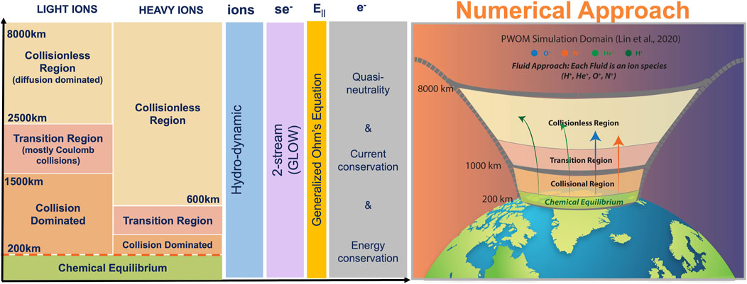
Polar Wind Outflow Model (PWOM) of Lin et al. (2020); Lin (2023) tracks the transport of electrons and seven ionospheric ion species (, , , , , , and ) from 200 km altitude up to a few and along high-latitude magnetic field lines, with 65 latitude or above (ranging auroral and cusp regions). From low to high altitudes, several altitude-dependent physical processes dominate over each region. For instance, at the inner boundary of the PWOM (200 km altitude), chemical and thermal equilibrium determine the number density and the temperature of each ion species. At a few hundred kilometers of altitude, the collisional process starts to dominate. Once reaching higher altitudes, diffusion becomes the dominant mechanism, and those regions are known as collisionless regions, as illustrated in Figure 1. Heavy and light ions, due to their mass differences, have their own boundary altitudes in collision, transition, and collisionless regions. Inheriting its numerical scheme from PWOM of Glocer et al. (2009, 2012); Glocer et al. (2017, 2018, 2020), the PWOM of Lin et al. (2020) solves the ions based on the gyrotropic transport equations, including the continuity, momentum, and energy equations. As shown in Figure 1, the thermal electron solution is derived from the assumption of quasi-neutrality and current and energy conservation (Gombosi and Nagy, 1989), while the Suprathermal Electron (SE) solution is obtained from the two-stream GLobal airglOW (GLOW) model (Solomon, 2017). Additionally, PWOM obtains the number density and temperature of the neutral atmosphere by either the NRLMSISE-00 (referred to as MSIS in this paper) empirical model (Picone et al., 2002) or the Global Ionosphere Thermosphere Model (GITM) (Ridley et al., 2006). Specifically, information of neutral O, H, , , and He is provided by MSIS, and the distributions of neutral NO and N (²D) are from the GITM.

FIGURE 1

Lin, 2023).

Ionospheric outflow is primarily produced in the ionosphere F layer through ionospheric chemistry and SE production, including photoionization and secondary electron impact, and ion-neutral-electron chemical reactions (André and Yau, 1997; Schunk and Nagy, 2009). The SE production rate of each ion species in PWOM is derived from the cross-sectional area of the neutral-electron collision (Gronoff et al., 2012b,a). On the other hand, an ionospheric chemistry table with 54 chemical reactions was included to solve the production and loss of ions in PWOM (Lin, 2023). These production mechanisms directly contribute to the source terms in the transport equations of PWOM, and they are associated with the information on the exosphere density. As discussed in Section 1, the charge exchange reaction rate between heavy and ions with neutral H are largely different in the ionosphere. The reaction rate of with neutral H is (), while the reaction rate of with neutral H is (), assuming electron temperature 3,000 K (Schunk and Nagy, 2009). With more than two orders of magnitude differences in the charge exchange reaction rates, the charge exchange between and H rapidly removes ions from the polar wind, but not ions.

Once ions are produced, they experience several energization mechanisms to escape from the ionosphere, such as ambipolar electric field, frictional heating, SE impact, and WPI. Since this study focuses on the ionospheric outflow during geomagnetically quiet time, the former two energization mechanisms will be investigated in Section 4. The ambipolar electric field, also known as the electron pressure gradient force, is developed in response to slight electron-ion charge separations in the topside ionosphere (Banks and Holzer, 1968; Banks, 1970; Banks and Kockarts, 1973). Although the ambipolar electric field is not sufficient to accelerate all the polar wind ions, especially for heavy and ions, this electric field exists at all altitudes and serves as a fundamental acceleration mechanism for all the high-latitude ionospheric outflow. Based on the ion and electron solutions, PWOM derives the ambipolar electric field from general Ohm’s law (Gombosi and Nagy, 1989). Frictional heating, on the other hand, involves collisional interactions between electrons or ions with neutrals and alters the ions through momentum and energy exchange rates (Schunk and Nagy, 2009). The momentum and energy exchange terms due to collisional processes are approximated as non-linear terms in PWOM based on the Chapman-Cowling collision integrals (Schunk and Nagy, 2009). Frictional heating favors the transfer of energy and momentum from the hotter to the cooler species and leads to different temperatures and velocities for each species. Thus, increasing or decreasing the neutral H density, which is assumed to be low-temperature and zero-velocity neutral species in PWOM, results in a direct impact on the momentum and energy exchange terms of frictional heating with polar wind ions.

2.2 Simulation configuration

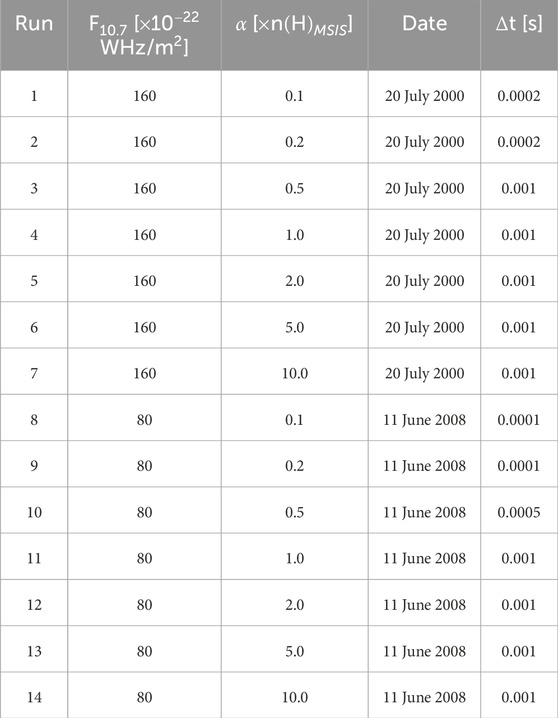
Table 1 shows the parameters, including solar radio flux , ratio applied to the neutral hydrogen density , and date, of 14 numerical simulations conducted in this study. The flux indicates the solar activity: the solar maximum is represented as 160 WHz/, and the solar minimum is 80 WHz/. Similarly, the dates were chosen during the summertime: the solar maximum summer is 20 July 2000, and the solar minimum summer is 11 June 2008. Figure 2 illustrates the variation of the neutral H density from MSIS based on both the solar flux and the date. In each simulation case, a steady-state single-field-line PWOM solution is obtained at the conclusion of an 8-hour-long simulation. This simulated field line is rooted and fixed at 80 latitude and 12 MLT in the northern hemisphere, presenting a local outflow solution near the high-latitude cusp region.

FIGURE 2

The design of the sensitivity analysis study was informed by available experimental evidence. Due to previous assessments of the uncertainty of the hydrogen exosphere being limited to the dayside ionosphere because of measurement contamination on auroral emissions (Waldrop and Paxton, 2013), the parameter study focused on evaluating the impact of hydrogen exosphere discrepancy specifically on the dayside, omitting consideration of plasma convection in the high-latitude ionosphere. In addition, the main controlling factor for a steady-state solution is the timing for ions to be produced in the ionosphere and transported to the high-altitude regions, which takes approximately 8 h in simulation time. All simulations were conducted for 24 h, and solutions for each hour were compared. Although different runs converged to the steady state at different rates, the simulated profiles with 8-h runs captured most features. Further simulations beyond 8 h only provided minor corrections.

To analyze the impact of uncertainty of the hydrogen exosphere to polar wind dynamics, a parameter study was defined: the neutral H density from MSIS is multiplied by 0.1, 0.2, 0.5, 1.0, 2.0, 5.0, and 10.0. Since neutral hydrogen densities obtained from MSIS overestimated those derived from Ly- data by a factor of 74% (Waldrop and Paxton, 2013), and underestimated those column-integrated intensities measured in H- by a factor of 33% (Nossal et al., 2012), the parameters of 0.5 and 2.0 mean to understand variations of ionospheric outflow within the error bar of exospheric densities (see Section 1). Other than understanding the uncertainty of the neutral hydrogen exosphere, the parameters of 10 and 0.1 are chosen to investigate the extreme conditions in which the hydrogen exosphere deviates by more than one order of magnitude or less than ten percent from present conditions. These choices are based on the belief that the escape of neutral hydrogen during the early Earth’s atmosphere was slower by two orders of magnitude than previously assumed (Tian et al., 2005).

All the PWOM simulations use a field-aligned grid spacing of 20 km and assume that the molecular ions are stationary species, in which the molecular ions have a constant temperature as the neutral species, and their densities are determined via chemical equilibrium. Additionally, t in Table 1 provides an optimized result of time steps chosen in each simulation and depends on the Courant number , which is the velocity. When the neutral hydrogen density has a small number, the plasma velocity is low, and therefore, a small time step helps stabilize the Courant–Friedrichs–Lewy (CFL) condition. As indicated in Table 1, the value of was primarily selected as , but it was occasionally set to or even in instances where the neutral hydrogen exosphere displayed a small number to prevent numerical instability.

2.3 Hydrogen density distributions

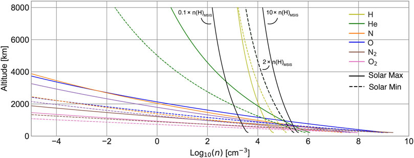
The altitude-dependent distribution of neutral hydrogen (H) densities in PWOM simulations is obtained from the NRLMSIS00 empirical model. To provide global neutral densities and temperature, MSIS uses several datasets, including total mass density derived from satellite accelerometers, temperature derived from incoherent scatter radar, and molecular oxygen estimations derived from solar ultraviolet emission, that are fitted to spherical harmonics functions (Hedin, 1991; Picone et al., 2002). Integrating the MSIS empirical model solution as a neutral atmosphere background to PWOM has been completed previously by Glocer et al. (2009). A wrapper has been built to convert the geographic coordinates in MSIS to GSM coordinates in PWOM. Since MSIS only provides neutral densities up to 1,000 km altitude, the neutral densities are assumed to decay by the scale height of the neutral species above. Figure 2 shows the neutral density background of PWOM simulations from MSIS during the Solar Maximum ( flux equals 160 WHz/, solid line), and Solar Minimum ( flux equals 80 WHz/, dashed line). Neutral N, O, , and are the main species in the low-altitude region, but their densities drastically decrease in the high altitudes. Neutral light H and He, in contrast, become the major species above 1,000 km altitude. Furthermore, neutral H densities of run 1, 7, 10, and 11 marked in Table 1 are shown as black lines in Figure 2. Those case comparisons will be further discussed in Section 4. Since the neutral temperatures in the Solar Maximum are larger than the Solar Minimum, the neutral atmosphere expands to higher-altitude regions. The increase of neutral temperatures leads to the enhancement of thermal escape. Therefore, neutral densities are larger during the Solar Minimum than the Solar Maximum in the low-altitude regions, while they are smaller during the Solar Maximum than the Solar Minimum in the high-altitude regions.

3 Impact of the terrestrial exosphere in ionospheric outflow

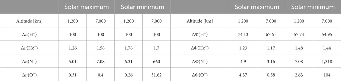
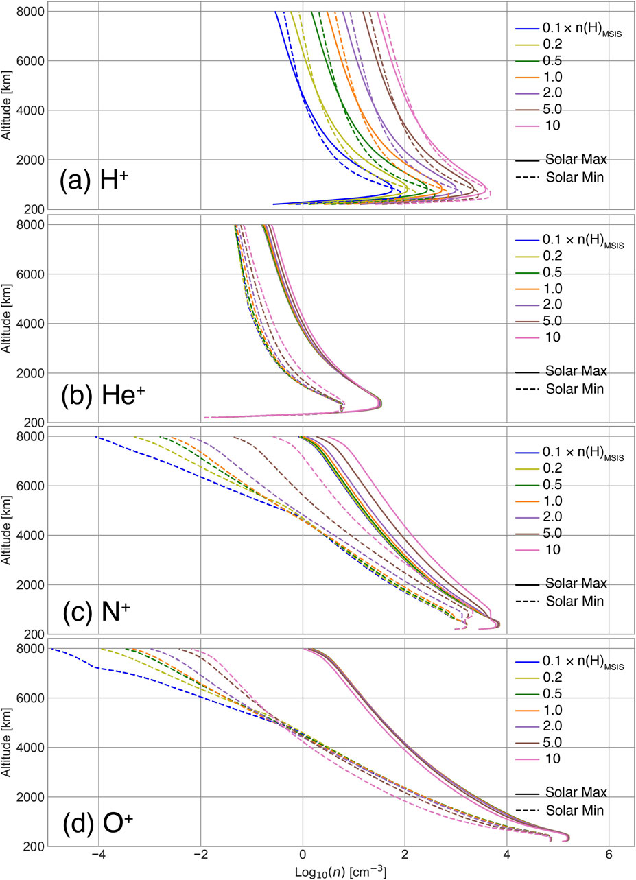
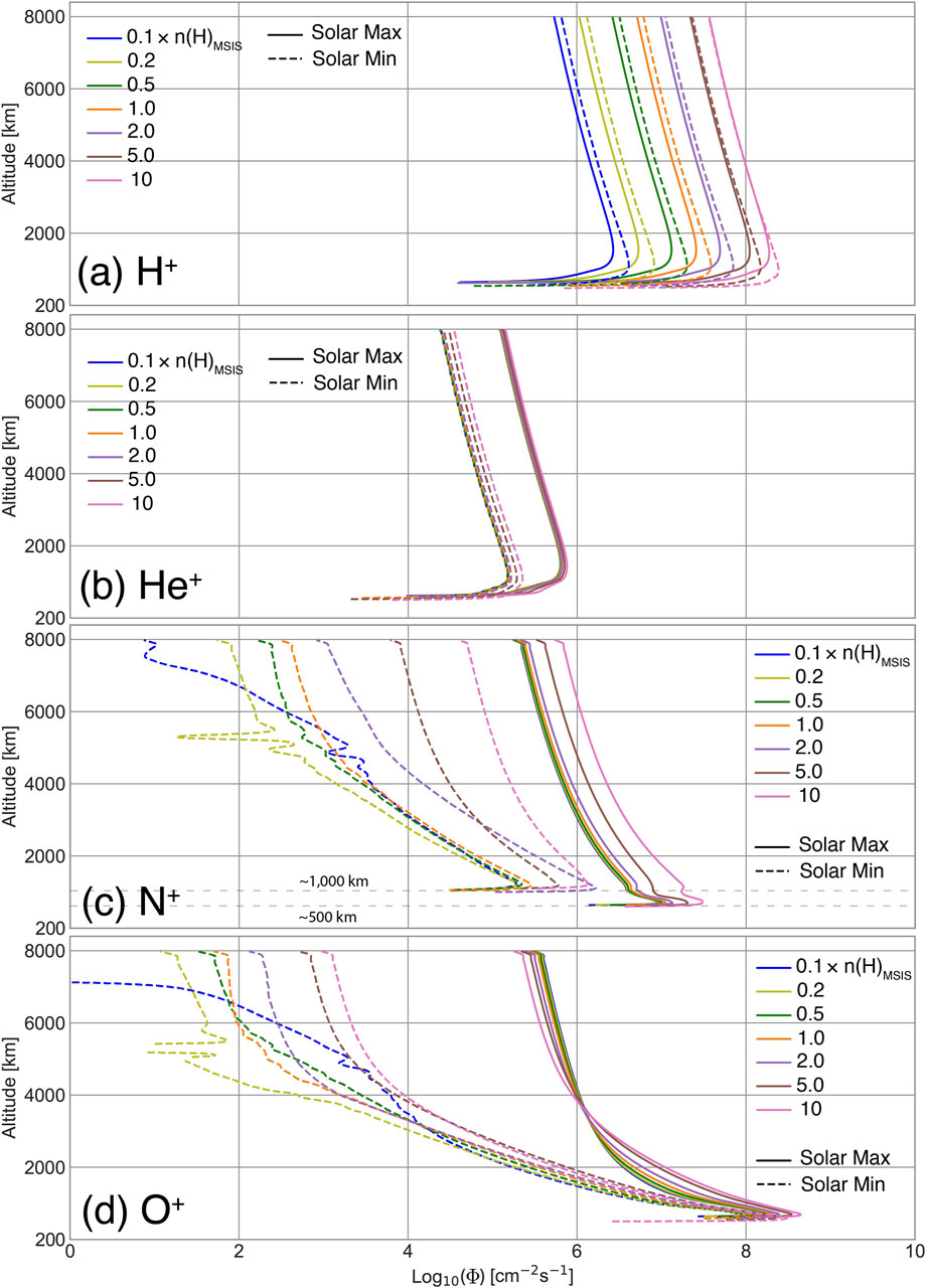
This section reports the variability of polar wind ion densities and fluxes in response to an enhanced and depleted H exosphere as defined in Table 2. Figures 3, 4 display , , , and densities and fluxes, both in scales, from 200 to 8,000 km altitude for all PWOM simulations, varied by different solar activities and neutral hydrogen densities. Ion fluxes are calculated based on the profiles of number densities and velocities from PWOM. The colors of lines represent cases of 0.1 (blue), 0.2 (light green), 0.5 (dark green), 1 (orange), 2 (purple), 5 (brown), and 10 (pink). Table 2 further quantifies the differences in densities and fluxes between 10n and 0.1n at 1,200 and 7,000 km altitude. and are calculated as follows:where is the ion species andThe reason to select 1,200 and 7,000 km altitude is due to the fact that ion transport to 1,200 km altitude typically forms the upflow populations, while ion transport to 7,000 km altitude will eventually become outflow populations (Zou et al., 2021; Godbole et al., 2022). Therefore, and at 1,200 and 7,000 km altitude provide a picture of how the upflow and outflow composition are altered by the hydrogen exosphere. Numbers in Table 2 mean to present the variations of ion densities and fluxes with different neutral hydrogen densities. Note that large numbers in Table 2, such as , are led by small values of and densities and fluxes.

FIGURE 3

FIGURE 4

3.1 Density variations

As shown in Figure 3A, density shows a linear relationship with neutral hydrogen density during both Solar Maximum and Minimum. This relationship is further supported by the data presented in Table 2, which demonstrates that a two-order of magnitude increase in H density (from 0.1 to 10n) corresponds to a two-order magnitude increase in density at both 1,200 and 7,000 km altitudes. That is, when increasing H density by a factor of , density always increases by a factor of . Moreover, solar activity significantly influences density, with the density being greater during the Solar Minimum compared to the Solar Maximum due to the augmented H density. Notably, the altitude, where density during the Solar Minimum surpasses that of the Solar Maximum, decreases from 5,000 to 3,000 km altitude when neutral H density varies from 0.1n (see blue solid and dashed lines in Figure 3A) to 10n (see pink solid and dashed lines in Figure 3A), indicating the strong dependence of the transition region boundary on the hydrogen exosphere.

Contrary to density, density (Figure 3B) shows minimal variations among the four ion species, indicating that the abundance of is not significantly dependent on the hydrogen exosphere. Although density decreases by an order of magnitude when transitioning from Solar Maximum to Solar Minimum, the overall density variations remain limited. As indicated in Table 2, during Solar Minimum, n () slightly increases from 1.26 to 1.56 at 1,200 km altitude and from 1.58 to 1.7 at 7,000 km altitude. Similarly, n () consistently remains less than two, regardless of solar activity and altitude.

Unlike and ions, heavy (Figure 3C) density is highly dependent on the neutral exosphere distribution and solar activity, and their variations are non-linear and altitude-dependent. density increases when 2, 5, and 10n, while it remains at similar magnitudes during 0.1, 0.2, 0.5 and 1n. Most importantly, density variations significantly increase during the Solar Minimum, even though its density generally decreases. As calculated in Table 2, increasing H density by two orders of magnitude during the Solar Maximum leads to the enhancement of density by a factor of 5 and 7 at 1,200 and 7,000 km altitude. During the Solar Minimum, n () is 6.31 at 1,200 km altitude but becomes 660 at 7,000 km altitude. These substantial variations in n () suggest that the hydrogen exosphere plays a more significant role in controlling density during the Solar Minimum as opposed to the Solar Maximum. Overall, during the Solar Maximum, density only increases slightly when H density increases by a factor of . However, density can increase by a similar factor at low altitudes and by more than two orders of magnitude at high altitudes during the Solar Minimum.

As seen in Figure 3D, is the only species whose density could decrease as H density increases, with density variations highly dependent on altitudes and solar activity. The decrease in abundances is primarily attributed to charge exchange interactions between and neutral H. As neutral hydrogen density increases, ions are predominantly lost through charge exchange reactions. Consequently, the density of ions in the low-altitude region, where their production primarily occurs, decreases when neutral hydrogen density increases. A more in-depth explanation of the charge exchange process between and neutral H and how this process differs from the profiles of and will be further discussed in Section 4. Table 2 displays that during the Solar Maximum, density with 10n is only 30%–40% of the density with 0.1n. However, during the Solar Minimum, density with 10n exceeds that with 0.1n by more than an order of magnitude. These differences between Solar Maximum and Minimum indicate that the mechanisms responsible for energizing become more significant during Solar Minimum as opposed to Solar Maximum. Overall, during Solar Maximum, density only decreases slightly when H density increases by a factor of . Conversely, during the Solar Minimum, density still decreases by a similar factor in the low-altitude region, but its abundance is enhanced by more than one order of magnitude in the high-altitude region.

3.2 Flux variations

Figure 4 shows the upflowing , , , and fluxes, which determine the ionospheric escape rates and highlight the influence of energization on the ionospheric outflow. Similar to the behavior of density (Figure 3A), an increase in neutral H density results in a linear enhancement of flux (Figure 4A). Unlike density, the flux during the Solar Minimum surpasses that during the Solar Maximum at all altitudes. This discrepancy is attributed to the substantial increase in production in low-altitude regions during the Solar Minimum, resulting from enhanced neutral H densities. As a consequence, the produced ions modify the energization processes of and consequently lead to higher velocities during the Solar Minimum compared to the Solar Maximum. Table 2 further indicates that the differences () are smaller than n () at all altitudes, and () are varied with the solar activity. Specifically, () are 74.13 and 67.13 during the Solar Maximum but only 57.74 and 54.95 at 1,200 and 7,000 km altitudes during the Solar Minimum. Meanwhile, n () remains at 100 for all cases. These differences between () and n () suggest that the energization mechanisms influencing are not linearly correlated with the production mechanisms of . On the other hand, flux (Figure 4B) generally mirrors its density profile (Figure 3B), with flux remaining at similar magnitudes as the neutral H density. The differences n () and () in Table 2 all range between 1 and 2, even as neutral H density increases by two orders of magnitude.

Both and fluxes (Figures 4C,D) exhibit fluctuations in the high altitude regions (4,000–6,000 km), particularly during the Solar Minimum with low neutral H density. These fluctuations occur when ions have insufficient energy to transition from upflow to outflow. Therefore, a portion of ion upflow becomes ion downflow, while the rest continues as ion upflow, leading to a small net flux. Similar to density, flux remains at a similar magnitude when 2n and increases by a factor 3–5 when 5 and 10n. When the solar activity shifts from the Solar Maximum to the Solar Minimum, the initial altitude with upflowing flux elevates from 500 km to approximately 1,000 km. This difference in upflowing altitude suggests that obtains less energy during the Solar Minimum than during the Solar Maximum, resulting in the upflow population occurring at a higher altitude during the Solar Minimum. Unlike and fluxes, flux is varied larger during the Solar Minimum than the Solar Maximum. Table 2 indicates that () with 10n at 7,000 km altitude is more than 3 orders of magnitude larger than () with 0.1n. This significant difference in () may result from the circumstances of flux fluctuation mentioned above, attributed to the low energy possessed by during the Solar Minimum. Nevertheless, the substantial value of () suggests that neutral hydrogen plays a more significant role in controlling outflow, particularly during the Solar Minimum.

The unique feature of Figure 3D, which stands out as the only species whose density decreases with increasing neutral H density, does not appear in flux of Figure 4D. Below 3,000 km altitude, flux consistently increases with increasing neutral H density. Above 3,000 km altitude, flux with 10n are the largest value among all the cases during the Solar Minimum but the smallest value during the Solar Maximum. () in Table 2 are 4.37 and 2.68 at 1,200 km altitude and 0.58 and 104 at 7,000 km altitude. This indicates that upflowing flux increases with neutral H density, but the outflowing flux does not. Interestingly, flux variations in response to dynamic hydrogen exosphere align with the concept of “fast” molecular ion outflow, which refers to the phenomenon that only molecular ions with significant velocities can escape from the ionosphere due to the rapid recombination of molecular , , and ions with electrons (Seki et al., 2019). The resemblance between flux and molecular ion outflow emphasizes the significance of the energization mechanisms of , particularly during the Solar Maximum.

When comparing the abundances of all ion species with different cases of neutral H density, it is noteworthy to point out that density and flux can surpass . While remains the dominant species in the low-altitude regions, it experiences significant loss at higher altitudes as neutral hydrogen density increases. Therefore, while dominates the high-altitude regions, emerges as the second most abundant species with 5 and 10n during the Solar Maximum, and 2, 5, and 10n during the Solar Minimum. Furthermore, the variations in flux and density between the Solar Maximum and Minimum with similar neutral hydrogen density are less pronounced compared to those of , suggesting that the density and flux ratios of / are larger during the Solar Minimum than the Solar Maximum.

4 Discussion

Section 3 demonstrates the sensitivity of ion densities and fluxes in response to neutral hydrogen densities. Specifically, the outflowing fluxes of heavy and are varied by one to two orders in the high-altitude regions when neutral H density increases by 2 orders of magnitude. This section investigates the production and energization schemes of each ion species to explain the ions’ density and flux variations. Two cases are compared in detail: (1) 1n vs. 2n during the Solar Minimum. This comparison aims to understand the impact of the uncertainty of the exospheric density (factor of 2) in the polar wind at present Earth conditions. (2) 0.1n vs. 10n during the Solar Maximum. Even though the neutral hydrogen densities in these two cases rarely happen, this comparison could estimate the composition of ionospheric outflow during hydrogen-poor and hydrogen-rich atmospheres. The latter is a typical case of early Earth conditions.

4.1 The response of polar wind dynamics to reported uncertainty in MSIS exosphere

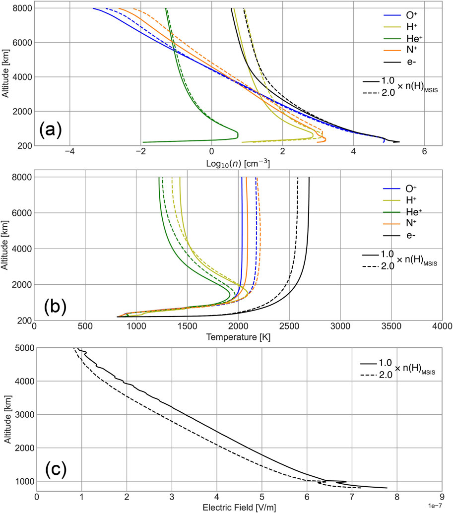
Figure 5 shows the ion density and temperature of , , and when neutral hydrogen density equals 1n and 2n during the Solar Minimum (run 11 and 12 of PWOM simulations highlighted in Table 1). When the exosphere density increases by a factor of 2, density and temperature exhibit enhancements. Meanwhile, temperature increases across all altitudes, with a slight decrease in density at lower altitudes and an increase at higher altitudes. density also increases from 1n to 2n; however, its temperature decreases above 4,000 km altitude. Notably, has a larger density and higher temperature than ions in the high-altitude region.

FIGURE 5

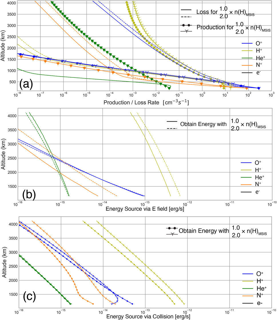
Figure 6A investigates the production and loss through ionospheric chemistry. When the neutral hydrogen density is doubled, the production rate of also doubles, while the production rates of other ions remain relatively unchanged. In contrast, the loss rates of and increase by a factor of 1.5–3. The production of and the loss of are credited to the charge exchange between and neutral H, which is one of the dominant chemical reactions in the ionosphere. Similarly, the loss of is also attributed to charge exchange between and neutral H. Furthermore, this study also highlights the importance of photoionization of in the supply of cold in the magnetosphere (Borovsky et al., 2022). As shown in Figure 6, the divergence of production (light green o- and Y- lines) and loss (blue solid and dashed lines) profiles in the high-altitude regions (beyond 2,000 km altitude) suggests that the photoionization of is effective to produce at the collisionless region. Overall, this production/loss profile shows that increasing the neutral hydrogen density from 1n to 2n leads to (a) an increase in density due to an increased production rate, and (b) an increase in the loss rates of and . However, the latter fact contradicts Figure 5A, which shows that and densities actually increase with neutral hydrogen densities. This inconsistency between density and production/loss profiles suggests that the energization of and may also be influenced by the hydrogen exosphere.

FIGURE 6

In Section 2, we discussed the various energization mechanisms included in PWOM. Among these mechanisms, ambipolar electric fields and frictional heating are identified as the most critical mechanisms driving ion energization above 500 km altitude during geomagnetically quiet times. Figure 6B and c depict the energization of ions due to ambipolar electric fields and frictional heating within the altitude range of 500–4,000 km. When the neutral H density is doubled, both heavy and experience increased energization through ambipolar electric fields and frictional heating. Specifically, the energy obtained by from both mechanisms increases by more than one order of magnitude, while only experiences a 1.five to three fold increase. This disparity in energization response between and based on neutral hydrogen density can be attributed to their relative abundances in the ionosphere. As the abundance of is consistently higher than in the low-altitude regions, is more likely to lose energy through frictional heating with other species than . Overall, the dissimilarity in the energization mechanisms of and suggests that / density and flux ratios can be altered by variations of neutral hydrogen exosphere.

Changes in the neutral hydrogen exosphere also impact ion energization through the ambipolar electric field. When the neutral hydrogen density doubles, the production rate and density of also double. This leads to an increase in electron density, which corresponds to the total ion density, by a factor of 2, as shown by the black lines in Figure 5A. To maintain total energy conservation, the increase in ion temperatures, as depicted in Figure 5B, implies a decrease in electron temperature, which is evident from the black lines in Figure 5. Additionally, the decrease in electron temperature causes a reduction in the ambipolar electric field, leading to a decrease of approximately 10%–20%, as illustrated in Figure 5C.

The production/loss profile depicted in Figure 6A suggests that ion losses, directly influenced by the neutral H exosphere, exert a more significant influence on controlling density variations than ion productions during Solar Minimum. In other words, during the Solar Maximum, when ion production rates through photoionization are larger, the ion losses through charge exchange with neutral H become less important. Thus, the density variations of ion densities and fluxes are smaller compared to those during the Solar Minimum, as illustrated in Figures 3, 4.

The findings of this comparison are consistent with prior research on low-latitude ionospheric outflow, which proposed a correlation between and neutral H densities due to rapid charge exchange between and neutral H (Krall et al., 2018). However, this study highlights that density variations in response to neutral H density during Solar Maximum are smaller than those during Solar Minimum, in contrast to the findings of Krall et al. (2018). This disparity suggests that the underlying production and energization mechanisms of low- and high-latitude ionospheric outflow may exhibit different responses to neutral H density. Two potential explanations for this disparity are: (a) the ambipolar electric field in high-latitude ionospheric outflow may efficiently energize more ions during Solar Maximum compared to Solar Minimum, and (b) the significant presence of heavy ions in the high-latitude ionospheric outflow could enhance outflow populations by modifying the collisional schemes in the ionosphere (Lin et al., 2020).

4.2 The response of polar wind dynamics to hydrogen-poor and hydrogen-rich atmospheres

Based on the evolution history of Earth’s atmosphere, high hydrogen concentration is known to create favorable environments for a habitable planet because it can provide greenhouse warming against the early Sun and allow molecules suitable for the origin of life to form (Urey, 1952; Tian et al., 2005). Unlike rocky planets in our solar system, the atmospheric compositions of Earth-like planets are largely unknown. Some planets may retain a hydrogen-rich atmosphere, while others experience fast H escape and become a hydrogen-poor atmosphere (Miller-Ricci et al., 2008). However, the knowledge of how the neutral hydrogen density facilitates the atmospheric escape from Earth-like planets remains unknown. Comparison of 0.1n vs. 10n provides a means to estimate the atmospheric loss rate with hydrogen-rich and hydrogen-poor atmosphere. In these simulations, the neutral compositions of present Earth’s atmosphere during the Solar Maximum have remained the same, but the neutral hydrogen density, which is a minor composition of the neutral atmosphere in the ionosphere, is defined as 0.1n and 10n to represent a hydrogen-poor and hydrogen-rich atmosphere, respectively. Although the neutral compositions of Earth and other exoplanets during the early phase of atmospheric evolution may not be the same as the present Earth’s neutral composition, the comparison of these simulations only helps assess the potential role of neutral hydrogen plays in the ionospheric escape.

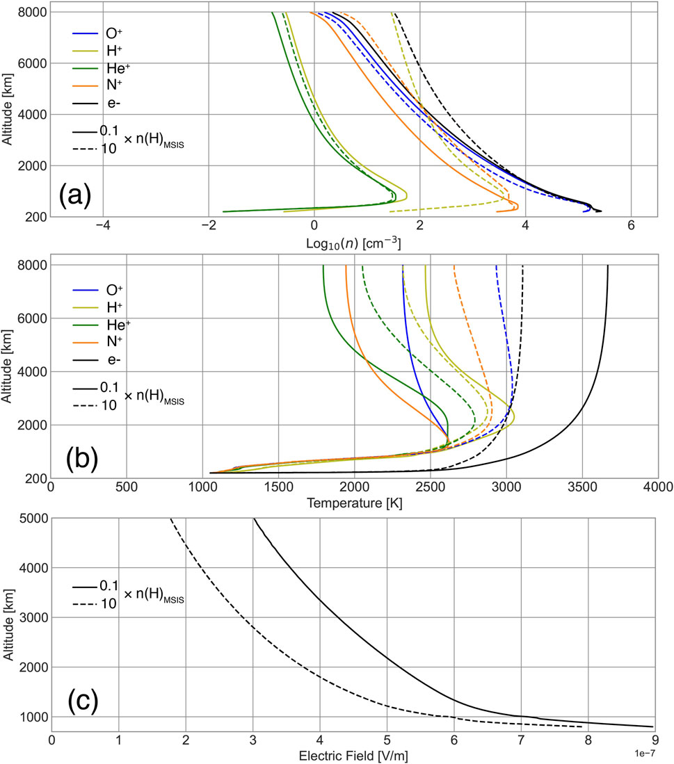
Changes in the ion and electron solutions, as well as the production and energization mechanisms, align with the trends presented in Section 4.1, but with significant differences in orders of magnitude. As depicted in Figure 7A, a two-order-of-magnitude increase in neutral hydrogen densities results in a 2-order-of-magnitude increase in density, a 2-fold increase in density, and an order-of-magnitude increase in density. In contrast, density decreases by a factor of 2. Additionally, Figure 7B illustrates that at an altitude of 8,000 km, the temperatures of and increase from 1,800 K to 2,100 K and from 2,300 K to 2,900 K, respectively, while temperature increases by approximately 40%, from nearly 2,000 K to 2,700 K. temperatures experience a slight decrease of up to 100 K, while temperatures drop from 3,700 K to 3,100 K, a decrease of approximately 20%. Figure 7C further shows that the ambipolar electric field is reduced by 10%–50% due to the overall increase of ion energization, as explained in Section 4.1.

FIGURE 7

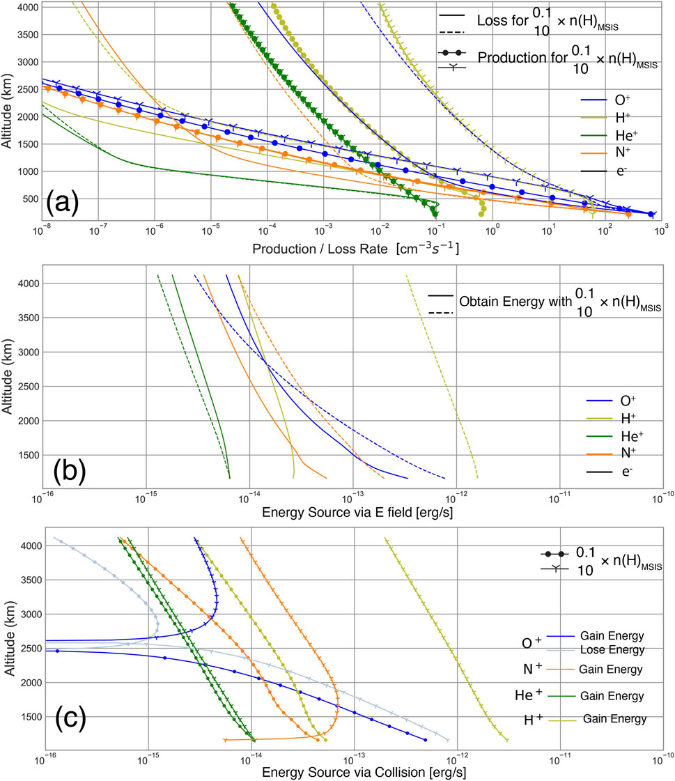
When neutral hydrogen densities increase by two orders of magnitude, we observe an enhancement of density and a deduction in density, which are both attributed to the production and loss mechanisms of ionosphere chemistry. As demonstrated in Figure 8A, the increase in neutral hydrogen densities results in a proportionate increase in loss rates, along with a rise in production rates by two orders of magnitude. This outcome is a result of the rapid charge exchange between and neutral H, as discussed in Section 2 and 4.1. Additionally, although production rates also escalate due to the charge exchange between and neutral O, their magnitudes are significantly lower than loss rates. This rapid charge exchange of with neutral H has an impact on the energization schemes of , as depicted in Figures 8B,C. When neutral hydrogen density equals 0.1n, ions gain energy through frictional heating from and electrons, which possess higher temperatures, and ambipolar electric field up to an altitude of 2,500 km. Above this altitude, begins to lose energy through frictional heating but still gains energy through the ambipolar electric field. Conversely, when neutral hydrogen density increases to 10n, the frequent charge exchange between and neutral H causes rapid energy loss of ions, resulting in a negative energy source for . Once reaching the high-altitude region (approximately 2,500 km altitude), begins to gain energy from other species through frictional heating.

FIGURE 8

ion density exhibits an increase of up to one order of magnitude when neutral hydrogen density transitions from 0.1n to 10n, whereas density decreases by a factor of 2. The contrasting trends in the density profiles of and ions result in density surpassing density in the high-altitude region, despite abundance being over one order of magnitude smaller than at lower altitudes. Analysis of Figures 8A,B, and c reveals that the augmented neutral hydrogen densities result in a one to three orders of magnitude increase in loss rates, but the energization of via ambipolar electric field and frictional heating intensifies by a factor of 5–10 at all altitudes. Consequently, ions are energized at a faster rate than , leading to larger temperature variations in , as indicated in Figure 7B, and become the dominant heavy ion species.

In conclusion, neutral hydrogen density determines the ionospheric outflow composition. In a hydrogen-poor atmosphere, the ion outflow is dominated by , whereas in a hydrogen-rich atmosphere, and become dominant. Moreover, the increase in electron density, which represents the total ion density, in the hydrogen-rich exosphere suggests that the transition altitude between the collision and collisionless regions extends to higher altitudes. The PWOM utilized in this study is capable of capturing this feature, as the density with 10n remains comparably significant up to an altitude of 1,000 km. This suggests that plays a pivotal role in a hydrogen-rich atmosphere, and its significant presence in the atmospheric escape may help assess the habitability of exoplanets, as nitrogen is an essential element to form the life and stabilize the liquid water on a planet’s surface (Schwieterman et al., 2015; Johnstone et al., 2018; Kislyakova et al., 2020). Additionally, and ions exhibit distinct pathways of energization under varying neutral hydrogen densities. While the energization of ions is closely associated with the charge exchange with neutral H, ions are more prone to acquiring energy from both ambipolar electric field and ion-neutral-electron collisions, facilitating their escape from the ionosphere.

5 Conclusion

This study provides a picture that the abundances of ionospheric outflow are not linearly correlated with neutral hydrogen density. While ions demonstrate a linear increase in abundance, variations in and densities and fluxes are mostly non-linear and are influenced by solar activity. Furthermore, increasing the H exosphere density leads to rapid charge exchange between and neutral H, but not for charge exchange between and neutral H. Therefore, abundance impedes when neutral hydrogen densities are greater than 5n during the Solar Maximum and 2n during the Solar Minimum, indicating that plays a more significant role in the ionospheric outflow with the dynamic hydrogen exosphere. It is important to point out that the ionospheric and profiles presented in this study do not consider the impact of collisions between neutral O and , which was advised as another limiting factor of their outflowing fluxes. Nevertheless, the outflow rate is mainly controlled by the neutral H density in the topside ionosphere and is unaffected by neutral O and collisions (Krall and Huba, 2019). Most importantly, the discrepancy between outflowing and solutions shown in this study highlights the need to measure and in Earth’s magnetosphere-ionosphere system, as their different behaviors are known to provide a better understanding of the production and energization mechanisms of heavy particles in response to geomagnetic storm activities (Ilie and Liemohn, 2016; Liu et al., 2022; Ilie et al., 2023; Krall et al., 2023). For example, / ratios are sensitive to the neutral atmosphere composition, including neutral O/ density ratios and neutral hydrogen density, leading to the fact that / ratios are varied by the solar activities, seasons, and geomagnetic storm activities (Lin et al., 2020; Albarran et al., 2024).

In the upcoming years, NASA Carruthers Geocorona Observatory will routinely image the terrestrial exosphere in Lyman-Alpha from the Sun-Earth Lagrange point L1 (Waldrop et al., 2023). This mission aims to provide global exospheric H densities from the ground up to 35 during solar maximum and medium conditions. This work built the foundations of ion-neutral coupling studies in the ionospheric outflow and will be further improved when global data-based H density becomes available. It is important to note that this study only scales the neutral H profile from MSIS by a fixed factor and does not account for its altitude-dependent distribution. However, the simulation results suggest a strong correlation between ionospheric outflow and the neutral exospheric H atoms. It further advises that ion-neutral reactions, which play an important role in regulating the plasma dynamics in Earth’s magnetosphere and ionosphere, require accurate knowledge of the hydrogen exosphere. Future directions of this work include (a) the analysis of the polar wind response to storm-time exospheric densities whose increase of up to 20% during these geomagnetically active periods have been previously reported in (Cucho-Padin and Waldrop, 2019; Zoennchen et al., 2017), (b) quantification of atmospheric escape that would include not only ion loss to space but also neutral H loss as ENAs due to charge exchange interactions, and (c) the use of realistic hydrogen densities derived from Ly- images acquired by the Carruthers Geocorona Observatory.

References

• 1

  AlbarranR. M.VarneyR. H.PhamK.LinD. (2024). Characterization of n+ abundances in the terrestrial polar wind using the multiscale atmosphere-geospace environment. J. Geophys. Res. Space Phys.129, e2023JA032311. 10.1029/.2023JA032311

  • CrossRef
  • Google Scholar
  • View reference in article

• 2

  AndréM.NorqvistP.AnderssonL.EliassonL.ErikssonA. I.BlombergL.et al (1998). Ion energization mechanisms at 1700 km in the auroral region. J. Geophys. Res. Space Phys.103, 4199–4222. 10.1029/97JA00855

  • CrossRef
  • Google Scholar
  • View reference in article

• 3

  AndréM.YauA. (1997). Theories and observations of ion energization and outflow in the high latitude magnetosphere. Space Sci. Rev.80, 27–48. 10.1007/978-94-009-0045-5_2

  • CrossRef
  • Google Scholar
  • View reference in article

• 4

  AxfordW. I. (1968). The polar wind and the terrestrial helium budget, 73, 68–55.

  • Google Scholar
  • View reference in article

• 5

  BaliukinI. I.BertauxJ.-L.QuémeraisE.IzmodenovV. V.SchmidtW. (2019). SWAN/SOHO lyman‐α mapping: the hydrogen geocorona extends well beyond the moon. J. Geophys. Res. Space Phys.124, 861–885. 10.1029/2018JA026136

  • CrossRef
  • Google Scholar
  • View reference in article

• 6

  BanksP. M. (1970). Plasma transport in the topside polar ionosphere. Polar Ionos. Magnetos. Process.193.

  • Google Scholar
  • View reference in article

• 7

  BanksP. M.HolzerT. E. (1968). The polar wind. polar wind73, 6846–6854. 10.1029/JA073i021p06846

  • CrossRef
  • Google Scholar
  • View reference in article

• 8

  BanksP. M.KockartsG. (1973). Aeronomy.(AERONOMY)

  • Google Scholar
  • View reference in article

• 9

  BashirM. F.IlieR. (2018). A new N⁺ band of electromagnetic ion cyclotron waves in multi-ion cold plasmas. Geophys. Res. Lett.45, 10150–10159. 10.1029/2018GL080280

  • CrossRef
  • Google Scholar
  • View reference in article

• 10

  BashirM. F.IlieR. (2021). The first observation of n+ electromagnetic ion cyclotron waves. J. Geophys. Res. Space Phys.126, e2020JA028716. 10.1029/2020JA028716

  • CrossRef
  • Google Scholar
  • View reference in article

• 11

  BishopJ. (1991). Analytic exosphere models for geocoronal applications. Planet. Space Sci.39, 885–893. 10.1016/0032-0633(91)90093-P

  • CrossRef
  • Google Scholar
  • View reference in article

• 12

  BorovskyJ. E.LiuJ.IlieR.LiemohnM. W. (2022). Charge-exchange byproduct cold protons in the earth’s magnetosphere. Front. Astronomy Space Sci.8, 785305. 10.3389/fspas.2021.785305

  • CrossRef
  • Google Scholar
  • View reference in article

• 13

  ChangT.CrewG. B.HershkowitzN.JasperseJ. R.RettererJ. M.WinninghamJ. D. (1986). Transverse acceleration of oxygen ions by electromagnetic ion cyclotron resonance with broad band left-hand polarized waves. Geophys. Res. Lett.13, 636–639. 10.1029/gl013i007p00636

  • CrossRef
  • Google Scholar
  • View reference in article

• 14

  Cucho-PadinG.FerradasC.WaldropL.FokM. C. H. (2020a). Understanding the role of exospheric density in the ring current recovery rate. AGU Fall Meet. Abstr.2020, SM037–09.

  • Google Scholar
  • View reference in article

• 15

  Cucho-PadinG.KamedaS.SibeckD. G. (2022). The earth’s outer exospheric density distributions derived from procyon/laica uv observations. J. Geophys. Res. Space Phys.127, e2021JA030211. 10.1029/2021JA030211

  • CrossRef
  • Google Scholar
  • View reference in article

• 16

  Cucho-PadinG.WaldropL. (2018). Tomographic estimation of exospheric hydrogen density distributions. J. Geophys. Res. Space Phys.123, 5119–5139. 10.1029/2018ja025323

  • CrossRef
  • Google Scholar
  • View reference in article

• 17

  Cucho-PadinG.WaldropL. (2019). Time-dependent response of the terrestrial exosphere to a geomagnetic storm. Geophys. Res. Lett.46, 11661–11670. 10.1029/2019gl084327

  • CrossRef
  • Google Scholar
  • View reference in article

• 18

  Cucho-PadinG.WaldropL.MaruyamaN. (2020b). Quantifying the impact of dynamic storm-time exospheric density on plasmaspheric refilling. AGU Fall Meet. Abstr.2020, SM040–0006.

  • Google Scholar
  • View reference in article

• 19

  GlocerA.DaldorffL. K. S. (2022). Connecting energy input with ionospheric upflow and outflow. J. Geophys. Res. Space Phys.127, e2022JA030635. 10.1029/2022JA030635

  • CrossRef
  • Google Scholar
  • View reference in article

• 20

  GlocerA.KhazanovG.LiemohnM. (2017). Photoelectrons in the quiet polar wind. J. Geophys. Res. Space Phys.122, 6708–6726. 10.1002/2017ja024177

  • CrossRef
  • Google Scholar
  • View reference in article

• 21

  GlocerA.KitamuraN.TothG.GombosiT. (2012). Modeling solar zenith angle effects on the polar wind. J. Geophys. Res. Space Phys.117, A04318. 10.1029/2011JA017136

  • CrossRef
  • Google Scholar
  • View reference in article

• 22

  GlocerA.TothG.FokM.-C. (2018). Including kinetic ion effects in the coupled global ionospheric outflow solution. J. Geophys. Res. Space Phys.123, 2851–2871. 10.1002/2018ja025241

  • CrossRef
  • Google Scholar
  • View reference in article

• 23

  GlocerA.TóthG.GombosiT.WellingD. (2009). Modeling ionospheric outflows and their impact on the magnetosphere, initial results. J. Geophys. Res. Space Phys.114, 5216. 10.1029/.2009JA014053

  • CrossRef
  • Google Scholar
  • View reference in article

• 24

  GlocerA.WellingD.ChappellC. R.TothG.FokM.-C.KomarC.et al (2020). A case study on the origin of near-earth plasma. J. Geophys. Res. Space Phys.125, e2020JA028205. 10.1029/2020JA028205

  • CrossRef
  • Google Scholar
  • View reference in article

• 25

  GodboleN. H.LessardM. R.KenwardD. R.FritzB. A.VarneyR.MichellR. G.et al (2022). Observations of ion upflow and 630.0 nm emission during pulsating aurora. Front. Phys.890. 10.3389/fphy.2022.997229

  • CrossRef
  • Google Scholar
  • View reference in article

• 26

  GombosiT. I.NagyA. F. (1989). Time-dependent modeling of field-aligned current-generated ion transients in the polar wind. J. Geophys. Res.94, 359–369. 10.1029/JA094iA01p00359

  • CrossRef
  • Google Scholar
  • View reference in article

• 27

  GronoffG.Simon WedlundC.MertensC. J.BarthélemyM.LillisR. J.WitasseO. (2012a). Computing uncertainties in ionosphere-airglow models: ii. the martian airglow. J. Geophys. Res. Space Phys.117. 10.1029/2011JA017308

  • CrossRef
  • Google Scholar
  • View reference in article

• 28

  GronoffG.Simon WedlundC.MertensC. J.LillisR. J. (2012b). Computing uncertainties in ionosphere-airglow models: I. electron flux and species production uncertainties for mars. J. Geophys. Res. Space Phys.117. 10.1029/2011JA016930

  • CrossRef
  • Google Scholar
  • View reference in article

• 29

  HedinA. E. (1991). Extension of the msis thermosphere model into the middle and lower atmosphere. J. Geophys. Res. Space Phys.96, 1159–1172. 10.1029/90JA02125

  • CrossRef
  • Google Scholar
  • View reference in article

• 30

  HodgesR. R. (1994). Monte Carlo simulation of the terrestrial hydrogen exosphere. J. Geophys. Res. Space Phys.99, 23229–23247. 10.1029/.94JA02183

  • CrossRef
  • Google Scholar
  • View reference in article

• 31

  IlieR.LiemohnM. W. (2016). The outflow of ionospheric nitrogen ions: a possible tracer for the altitude-dependent transport and energization processes of ionospheric plasma. J. Geophys. Res. Space Phys.121, 9250–9255. 10.1002/.2015JA022162

  • CrossRef
  • Google Scholar
  • View reference in article

• 32

  IlieR.LinM.-Y.BashirM. F.MajumderA. (2023). A review of n+ observations in the ionosphere-magnetosphere system. Front. Astronomy Space Sci.10, 1224659. 10.3389/fspas.2023.1224659

  • CrossRef
  • Google Scholar
  • View reference in article

• 33

  JohnstoneC. P.GüdelM.LammerH.KislyakovaK. G. (2018). Upper atmospheres of terrestrial planets: carbon dioxide cooling and the earth’s thermospheric evolution. Astronomy & Astrophysics617, A107. 10.1051/0004-6361/201832776

  • CrossRef
  • Google Scholar
  • View reference in article

• 34

  JoshiP. P.PhalY. D.WaldropL. S. (2019). Quantification of the vertical transport and escape of atomic hydrogen in the terrestrial upper atmosphere. J. Geophys. Res. Space Phys.124, 10468–10481. 10.1029/2019ja027057

  • CrossRef
  • Google Scholar
  • View reference in article

• 35

  KamedaS.IkezawaS.SatoM.KuwabaraM.OsadaN.MurakamiG.et al (2017). Ecliptic North-South symmetry of hydrogen geocorona. Geophys. Res. Lett.44 (11), 706. 10.1002/2017gl075915

  • CrossRef
  • Google Scholar
  • View reference in article

• 36

  KislyakovaK.JohnstoneC.ScherfM.HolmströmM.AlexeevI.LammerH.et al (2020). Evolution of the earth’s polar outflow from mid-archean to present. J. Geophys. Res. Space Phys.125, e2020JA027837. 10.1029/2020ja027837

  • CrossRef
  • Google Scholar
  • View reference in article

• 37

  KrallJ.FokM.-C.HubaJ. D.GlocerA. (2023). Stormtime ring current heating of the ionosphere and plasmasphere. J. Geophys. Res. Space Phys.128, e2022JA030390. 10.1029/.2022JA030390

  • CrossRef
  • Google Scholar
  • View reference in article

• 38

  KrallJ.GlocerA.FokM.-C.NossalS. M.HubaJ. D. (2018). The unknown hydrogen exosphere: space weather implications. Space weather16, 205–215. 10.1002/2017SW001780

  • CrossRef
  • Google Scholar
  • View reference in article

• 39

  KrallJ.HubaJ. (2019). The effect of oxygen on the limiting h+ flux in the topside ionosphere. J. Geophys. Res. Space Phys.124, 4509–4517. 10.1029/2018ja026252

  • CrossRef
  • Google Scholar
  • View reference in article

• 40

  LeeJ. H.BlumL. W.ChenL. (2021). On the impacts of ions of ionospheric origin and their composition on magnetospheric emic waves. Front. Astronomy Space Sci.8, 719715. 10.3389/fspas.2021.719715

  • CrossRef
  • Google Scholar
  • View reference in article

• 41

  LinM.-Y. (2023). Transport and energization of heavy ions in earth’s high latitude ionosphere. Phd thesis. Urbana, IL: University of Illinois at Urbana-Champaign. Available at: https://hdl.handle.net/2142/121964.

  • Google Scholar
  • View reference in article

• 42

  LinM.-Y.IlieR.GlocerA. (2020). The contribution of n+ ions to earth’s polar wind. Geophys. Res. Lett.47, e2020GL089321. 10.1029/2020GL089321

  • CrossRef
  • Google Scholar
  • View reference in article

• 43

  LiuJ.IlieR.BorovskyJ. E.LiemohnM. W. (2022). A new mechanism for early-time plasmaspheric refilling: the role of charge exchange reactions in the transport of energy and mass throughout the ring current—plasmasphere system. J. Geophys. Res. Space Phys.127, e2022JA030619. 10.1029/2022JA030619

  • CrossRef
  • Google Scholar
  • View reference in article

• 44

  McComasD. J.AllegriniF.BaldonadoJ.BlakeB.BrandtP. C.BurchJ.et al (2009). The two wide-angle imaging neutral-atom spectrometers (TWINS) NASA mission-of-opportunity. Space Sci. Rev.142, 157–231. 10.1007/s11214-008-9467-4

  • CrossRef
  • Google Scholar
  • View reference in article

• 45

  Miller-RicciE.SeagerS.SasselovD. (2008). The atmospheric signatures of super-earths: how to distinguish between hydrogen-rich and hydrogen-poor atmospheres. Astrophysical J.690, 1056–1067. 10.1088/0004-637x/690/2/1056

  • CrossRef
  • Google Scholar
  • View reference in article

• 46

  MooreT. E.FokM. C.ChandlerM. O.ChappellC. R.ChristonS. P.DelcourtD. C.et al (2005). Plasma sheet and (nonstorm) ring current formation from solar and polar wind sources. J. Geophys. Res. Space Phys.110, A02210. 10.1029/.2004JA010563

  • CrossRef
  • Google Scholar
  • View reference in article

• 47

  NossalS. M.MierkiewiczE. J.RoeslerF. L. (2012). Observed and modeled solar cycle variation in geocoronal hydrogen using NRLMSISE-00 thermosphere conditions and the bishop analytic exosphere model. J. Geophys. Res. Space Phys.117. 10.1029/2011ja017074

  • CrossRef
  • Google Scholar
  • View reference in article

• 48

  OuelletteJ. E.BramblesO. J.LyonJ. G.LotkoW.RogersB. N. (2013). Properties of outflow-driven sawtooth substorms. J. Geophys. Res. Space Phys.118, 3223–3232. 10.1002/jgra.50309

  • CrossRef
  • Google Scholar
  • View reference in article

• 49

  PeroomianV.El-AlaouiM.BrandtP. (2011). The ion population of the magnetotail during the 17 april 2002 magnetic storm: large-scale kinetic simulations and image/hena observations. J. Geophys. Res. Space Phys.116. 10.1029/.2010JA016253

  • CrossRef
  • Google Scholar
  • View reference in article

• 50

  PiconeJ. M.HedinA. E.DrobD. P.AikinA. C. (2002). Nrlmsise-00 empirical model of the atmosphere: statistical comparisons and scientific issues. J. Geophys. Res. Space Phys.107, 15–16. 10.1029/2002JA009430

  • CrossRef
  • Google Scholar

• 51

  QinJ.WaldropL. (2016). Non-thermal hydrogen atoms in the terrestrial upper thermosphere. Nat. Commun.7, 13655. 10.1038/ncomms13655

  • CrossRef
  • Google Scholar

• 52

  RegoliL. H.GkioulidouM.OhtaniS.RaptisS.MouikisC. G.KistlerL. M.et al (2024). Temporal evolution of o+ population in the near-earth plasma sheet during geomagnetic storms as observed by the magnetospheric multiscale mission. J. Geophys. Res. Space Phys.129, e2023JA032203. 10.1029/2023JA032203

  • CrossRef
  • Google Scholar

• 53

  RidleyA. J.DengY.TóthG. (2006). The global ionosphere thermosphere model. J. Atmos. Solar-Terrestrial Phys.68, 839–864. 10.1016/j.jastp.2006.01.008

  • CrossRef
  • Google Scholar

• 54

  SchunkR.NagyA. (2009). Ionospheres. second edn.Cambridge Books Online: Cambridge University Press.

  • Google Scholar

• 55

  SchwietermanE. W.RobinsonT. D.MeadowsV. S.MisraA.Domagal-GoldmanS. (2015). Detecting and constraining n2 abundances in planetary atmospheres using collisional pairs. Astrophysical J.810, 57. 10.1088/0004-637x/810/1/57

  • CrossRef
  • Google Scholar

• 56

  SekiK.KeikaK.KasaharaS.YokotaS.HoriT.AsamuraK.et al (2019). Statistical properties of molecular ions in the ring current observed by the arase (erg) satellite. Geophys. Res. Lett.46, 8643–8651. 10.1029/2019gl084163

  • CrossRef
  • Google Scholar

• 57

  ShayM. A.DrakeJ. F.SwisdakM.RogersB. N. (2004). The scaling of embedded collisionless reconnection. Phys. Plasmas11, 2199–2213. 10.1063/1.1705650

  • CrossRef
  • Google Scholar

• 58

  SolomonS. C. (2017). Global modeling of thermospheric airglow in the far ultraviolet. J. Geophys. Res. Space Phys.122, 7834–7848. 10.1002/2017JA024314

  • CrossRef
  • Google Scholar

• 59

  TianF.ToonO. B.PavlovA. A.De SterckH. (2005). A hydrogen-rich early earth atmosphere. Science308, 1014–1017. 10.1126/science.1106983

  • CrossRef
  • Google Scholar

• 60

  Toledo-RedondoS.AndréM.AunaiN.ChappellC. R.DargentJ.FuselierS. A.et al (2021). Impacts of ionospheric ions on magnetic reconnection and earth’s magnetosphere dynamics. Rev. Geophys.59, e2020RG000707. 10.1029/2020RG000707

  • CrossRef
  • Google Scholar

• 61

  UreyH. C. (1952). On the early chemical history of the earth and the origin of life. Proc. Natl. Acad. Sci.38, 351–363. 10.1073/pnas.38.4.351

  • CrossRef
  • Google Scholar

• 62

  VarneyR. H.WiltbergerM.ZhangB.LotkoW.LyonJ. (2016). Influence of ion outflow in coupled geospace simulations: 1. physics-based ion outflow model development and sensitivity study. J. Geophys. Res. Space Phys.121, 9671–9687. 10.1002/2016JA022777

  • CrossRef
  • Google Scholar

• 63

  WaldropL.ImmelT. J.ClarkeJ. T.JoshiP.WidloskiE.ZhangA.et al (2023). The carruthers geocorona observatory: a new era for exospheric sensing at earth. AGU Fall Meet. Abstr.

  • Google Scholar

• 64

  WaldropL.PaxtonL. J. (2013). Lyman α airglow emission: implications for atomic hydrogen geocorona variability with solar cycle. J. Geophys. Res. Space Phys.118, 5874–5890. 10.1002/jgra.50496

  • CrossRef
  • Google Scholar

• 65

  WalshB. M.PhanT. D.SibeckD. G.SouzaV. M. (2014). The plasmaspheric plume and magnetopause reconnection. Geophys. Res. Lett.41, 223–228. 10.1002/2013GL058802

  • CrossRef
  • Google Scholar

• 66

  WangX.ChenY.TóthG. (2022). Simulation of magnetospheric sawtooth oscillations: the role of kinetic reconnection in the magnetotail. Geophys. Res. Lett.49, e2022GL099638. 10.1029/.2022GL099638

  • CrossRef
  • Google Scholar

• 67

  ZoennchenJ. H.NassU.FahrH. J. (2015). Terrestrial exospheric hydrogen density distributions under solar minimum and solar maximum conditions observed by the TWINS stereo mission. Ann. Geophys.33, 413–426. 10.5194/angeo-33-413-2015

  • CrossRef
  • Google Scholar

• 68

  ZoennchenJ. H.NassU.FahrH. J.GoldsteinJ. (2017). The response of the H geocorona between 3 and 8 R_e to geomagnetic disturbances studied using TWINS stereo Lyman-α data. Ann. Geophys.35, 171–179. 10.5194/angeo-35-171-2017

  • CrossRef
  • Google Scholar

• 69

  ZouS.RenJ.WangZ.SunH.ChenY. (2021). Impact of storm-enhanced density (sed) on ion upflow fluxes during geomagnetic storm. Front. Astronomy Space Sci.8, 746429. 10.3389/fspas.2021.746429

  • CrossRef
  • Google Scholar

References

Albarran, R. M., Varney, R. H., Pham, K., and Lin, D. (2024). Characterization of n+ abundances in the terrestrial polar wind using the multiscale atmosphere-geospace environment. J. Geophys. Res. Space Phys. 129, e2023JA032311. doi:10.1029/.2023JA032311
CrossRef Full Text | Google Scholar