Models for plasmasphere and plasmatrough density and average ion mass including dependence on L, MLT, geomagnetic activity, and phase of the solar cycle

Using observations of mass density inferred from standing Alfvén wave frequencies and electron density inferred from plasma wave frequencies, predominantly for the Combined Release and Radiation Effects Satellite (CRRES) and Van Allen Probes spacecraft, we used symbolic nonlinear regression to find analytical formulas for the equatorial electron density, $n_{\text{e}}$, mass density, ${\rho }_{\text{m}}$, and average ion mass, $M\equiv {\rho }_{\text{m}}/n_{\text{e}}$. We separate the data into plasmasphere and plasmatrough populations based on the observed values of $n_{\text{e}}$ in order to find formulas for plasmasphere, plasmatrough, and both plasmasphere and plasmatrough. Our models depend on position, the solar extreme ultraviolet (EUV) F10.7 flux, geomagnetic activity parameters such as Kp, AE, Dst, and the solar wind dynamic pressure. Formulas for $M$ are presented with or without $n_{\text{e}}$ as an input parameter. By examining formulas of varying complexity, we are able to determine the relative importance of the various dependencies. The most important dependencies for $n_{\text{e}}$ and ${\rho }_{\text{m}}$ are that they decrease with respect to $L$ shell and geomagnetic activity as specified by parameters such as Kp. The most important dependence of $M$ is that $M$ increases with respect to increasing F10.7. The value of $M$ is close to unity within the plasmasphere, but can be significantly above 1 in the plasmatrough. Although $n_{\text{e}}$ and ${\rho }_{\text{m}}$ have maximum value at dusk local time, $M$ has maximum value at dawn local time. The O+ concentration is larger at dawn local time, but the O+ density can be comparable at dawn and dusk because of larger $n_{\text{e}}$ at dusk.

1 Introduction

Mass density, ${\rho }_{\text{m}}$, determines the timescale of low-frequency magnetohydrodynamic (MHD) phenomena in the magnetosphere and also affects ion-scale waves at frequencies near the ion gyrofrequency such as electromagnetic ion cyclotron (EMIC) waves (Denton et al., 2014a). In combination with the electron density, $n_{\text{e}}$, it can be used to calculate the average ion mass,

$M\equiv {\rho }_{\text{m}}/n_{\text{e}}.(1)$

While the exact composition of ions cannot be determined from $M$ alone, $M$ can lead to reasonable estimates of magnetospheric O+ concentration. There are two reasons for this. First of all, the He+ density is usually small relative to the H+ density (10% or less) (Craven et al., 1997; Fraser et al., 2005; Grew et al., 2007; Krall et al., 2008). Secondly, because of its greater mass, O+ affects mass density much more strongly than He+.

Assuming an H+/He+/O+/e plasma, if the He+ light ion concentration is (Denton et al., 2011)

${ϵ}_{\mathrm{H}\mathrm{e}}=n_{\mathrm{H}\mathrm{e}+}/\left(n_{\mathrm{H}+}+n_{\mathrm{H}\mathrm{e}+}\right),(2)$

then based on ${\rho }_{\text{m}}=n_{\text{H}+}+4n_{\text{He}+}+16n_{\text{O}+}$ (in amu per volume) and $n_{\text{e}}=n_{\text{H}+}+n_{\text{He}+}+n_{\text{O}+}$ (from quasi-neutrality), the O+ density will be.

$n_{\text{O}+}=n_{\text{e}}\frac{M-\left(1+3{ϵ}_{\text{He}}\right)}{16-\left(1+3{ϵ}_{\text{He}}\right)},(3)$

given that we have evaluated $M$ from Equation 1. Typically, for $L\ge 3.25$ that we consider in this paper, ${ϵ}_{\text{He}}$ will be limited to values less than about 0.1 (Craven et al., 1997). And unless $M$ is significantly greater than unity, $n_{\text{O}+}$ will be much less than $n_{\text{e}}$.

Denton et al. (2022) modeled ${\rho }_{\text{m}}$ and $M$ in the magnetosphere between $L=$ 1.3 and 10 for all conditions (although most of their data were for $L\ge 3$). But the magnetosphere can often be divided into a region of high electron density called the plasmasphere and a region of low electron density outside the plasmasphere called the plasmatrough. Because the properties of these two regions are very different, it is useful to have models for ${\rho }_{\text{m}}$ and $M$ in these two regions. For instance, it is well-known that whistler hiss waves occur dominantly in the plasmasphere, whereas whistler chorus waves occur predominantly in the plasmatrough (Millan and Thorne, 2007).

The boundary between the plasmasphere and plasmatrough is called the plasmapause (Carpenter and Anderson, 1992). But the plasmapause position can be very dynamic (Goldstein and Sandel, 2005), and there are even times for which no clear plasmapause exists (Denton et al., 2004). Nevertheless, we argue that we can divide the magnetospheric density measurements into “plasmasphere-like” and “plasmatrough-like” data based on the value of the electron density (Section 2.2). Whereas the plasmapause position is notoriously difficult to model or even describe, the electron density at the midpoint of the plasmapause is easier to model (Denton et al., 2024).

Models for electron density in the plasmasphere and plasmatrough (Carpenter and Anderson, 1992; Sheeley et al., 2001; Lv et al., 2022) yield higher density in the plasmasphere, but studies combining electron density and mass density suggest that there are more heavy ions in the plasmatrough (Takahashi et al., 2006; 2008; Denton et al., 2014b; Del Corpo et al., 2022). Thus we expect that ${\rho }_{\text{m}}$ will be higher in the plasmasphere, because of greater overall density, but that $M$ will be higher in the plasmatrough.

In this paper, we will use spacecraft observations of standing Alfvén wave frequencies to infer ${\rho }_{\text{m}}$ and simultaneous spacecraft observations of plasma wave frequencies to infer $n_{\text{e}}$. Then we will model $n_{\text{e}}$, ${\rho }_{\text{m}}$, and $M$ for separate plasmasphere and plasmatrough populations. Because we will use measurements from wave data rather than particle measurements [which most often cannot measure cold particles (Maldonado et al., 2023)], we expect to determine information about the total plasma density and composition in the plasmasphere and plasmatrough.

Our data analysis is similar to that of (Del Corpo et al., 2022), who used ground-based measurements of Alfvén frequencies to infer ${\rho }_{\text{m}}$ and simultaneous values of $n_{\text{e}}$ inferred from the Van Allen Probes to infer $M$ for times when the ground and space locations were approximately on the same field line. For determination of ${\rho }_{\text{m}}$, their approach has the advantage that data will almost always be available.

Our approach has two advantages. First, for measurements using spacecraft near the magnetic equator, mapping to the equator is a rather minor issue in comparison to mapping from ground locations, especially at large $L$. Second, because we use values of ${\rho }_{\text{m}}$ and $n_{\text{e}}$ found at the same spacecraft location, we do not have to worry about conjunctions. This means that our simultaneous values of ${\rho }_{\text{m}}$ and $n_{\text{e}}$ will be more accurate, and we will have much more data for a statistical study of $M$.

Other empirical studies have modeled magnetospheric density, particularly the electron density (Carpenter and Anderson, 1992; Sheeley et al., 2001; Lv et al., 2022). But our technique using symbolic nonlinear genetic regression is better able to determine independent dependencies involving many variables.

Another approach would be a neural network model (Chu et al., 2017; Zhelavskaya et al., 2017; Huang et al., 2022). That might yield somewhat more accurate models, but it is often difficult to interpret those results, whereas our method yields models with analytical equations.

Our models are expressed in terms of state variables, many of which are averages of some quantity over an interval of time. Possibly better models could result from timeseries analysis (Kondrashov et al., 2014), though again, the results would be more difficult to interpret.

This study is an empirical study. It is possible that physics based models (Maruyama et al., 2016; Jorgensen et al., 2017; Krall and Huba, 2021) for magnetospheric density could yield better results for event studies. But physics based models are not always more accurate, and empirical models are needed for baseline results in any case. See the review of density models by Ripoll et al. (2023).

In Section 2 we discuss the data used in this study and our methods, and in Section 3 we discuss our results. Discussion and conclusions follow in Section 4.

2 Data and methods

2.1 Spacecraft

We used data from the Combined Release and Radiation Effects Satellite (CRRES) and both Van Allen Probes (or Radiation Belt Storm Probes, RBSP-A and RBSP-B). These spacecraft had similar low inclination orbits. CRRES had an apogee of 6.2 $R_{\text{E}}$, whereas RBSP had an apogee of 5.8 $R_{\text{E}}$. CRRES operated in 1990 and 1991 during a strong solar maximum. RBSP operated between 2012 and 2019, which included a sampling of the rising phase of the solar cycle, a weak solar maximum, and solar minimum. Despite the differences in the conditions, our method, nonlinear symbolic regression (Section 2.5), will allow us to use the combined data to generate models, because the dependence on individual parameters will be determined independently.

Although both CRRES and RBSP had small apogees $\le 6.2$ $R_{\text{E}}$, there were some measurements at higher $L$ due to the combination of the inclination of the orbits and the dipole tilt (Figure 1B).

Figure 1

Figure 1. Distribution of observations. Occurrence distributions with respect to (A) year, (B) $L$, (C) F10.7 in sfu, (D) ${\text{Kp}}_{3\text{day}}$ (E) MLT in h, and (F) $n_{\text{e}}$ in ${\text{cm}}^{-3}$ for the (A) plasmasphere and (B) plasmatrough data sets. Here, and in similar figures, an uppercase letter stands for a row of panels and a lowercase letter stands for a column of panels.

Because we need $n_{\text{e}}$ to determine whether a particular measurement is in the plasmasphere or plasmatrough, as described below in Section 2.2, we limited our data to times at which we determined both ${\rho }_{\text{m}}$ and $n_{\text{e}}$. Denton et al. (2022) estimated uncertainties for ${\rho }_{\text{m}}$ of approximately 22%, and uncertainties of $n_{\text{e}}$ of approximately 20%.

Because of the much greater time span of measurements for RBSP, and because there were two RBSP spacecraft, we had much more data for RBSP than for CRRES. In order to give the data from CRRES, sampling a strong solar maximum, a better probability of influencing our models, we replicated each of the CRRES measurements three times (Our method, as described in Section 2.5, did not allow us to assign weights to the data points. Replication of data is essentially a manual way of doing weighting. The choice of three times increased the effect of the CRRES Measurements while still keeping the number of measurements small compared to those from the Van Allen probes).

The values of ${\rho }_{\text{m}}$ were determined from frequencies of Alfvén waves, and the values of $n_{\text{e}}$ were determined from the electron plasma wave frequency. The methods involved were described by Denton et al. (2022). A small number of measurements by CRRES, however, were removed from the database of Denton et al. (2022), because they were found to have values of ${\rho }_{\text{m}}$ inconsistent with those of $n_{\text{e}}$. Another difference is that we are now using a larger set of data for the Van Allen probes, which is described by Takahashi (2023).

Denton et al. (2022) also used data from the Time History of Events and Macroscale Interactions during Substorms (THEMIS) spacecraft. However, when we examined the plasmasphere data for the THEMIS spacecraft, we found that many of the inferred electron density values (found from the spacecraft potential) were unrealistically high compared to the inferrred values of mass density. So we decided for this study to only use data with plasma frequency measurements, generally considered to provide the best measure of total electron density.

For a model of ${\rho }_{\text{m}}$ using both plasmasphere and plasmatrough data, we also added additional data from the Geostationary Operational Environmental Satellites (GOES), the Active Magnetospheric Particle Tracer Explorers/Charge Composition Explorer (AMPTE/CCE), Geotail, and the Time History of Events and Macroscale Interactions during Substorms (THEMIS) spacecraft. Since this is a minor part of our study, we refer description of that data to that of Denton et al. (2022).

We combined simultaneous values of ${\rho }_{\text{m}}$ inferred from Alfvén frequencies of different harmonics for the Van Allen Probes and for THEMIS, using a weight for each measurement of mass density of ${(f_1/(d{f}_1\cdot {\rho }_{\text{m}1}))}^2$, where $f_1$, $d{f}_1$, and ${\rho }_{\text{m}1}$ are the frequency, frequency uncertainty, and inferred mass density for one particular harmonic. This weighting is based on standard error analysis (Lyons, 1991) assuming ${\rho }_{\text{m}1}\propto 1/f_1^2$ [because the Alfvén frequency is proportional to the Alfvén velocity $\propto {\rho }_{\text{m}}^{-1/2}$ (Denton et al., 2022)]. Given the same $d{f}_1$, higher frequency harmonics will have a higher weight because $d{f}_1/f_1$ is smaller (This procedure would also be useful for the GOES data, but we did not do that because the larger database using the GOES data plays a minor role in this study, as mentioned above. We used this procedure for THEMIS because originally we planned to use the THEMIS data for plasmasphere and plasmatrough results).

2.2 Plasmapause model

In our study, $L$ is defined as the maximum radius to any point on a magnetospheric magnetic field line using the TS05 magnetic field model (Tsyganenko and Sitnov, 2005), $R_{\text{max,TS}05}$, divided by the radius of the earth, $R_{\text{E}}$.

Denton et al. (2024) used electron density measurements from plasma wave data to find the electron density at the midpoint of the plasmapause, $n_{\text{e,pp}}$. We use their model 14 as a boundary value between “plasmasphere-like” populations and “plasmatrough-like” populations,

${\log }_{10}\left(n_{\text{e,pp}}\right)=-0.1193\left(\mathrm{c}\mathrm{M}\mathrm{L}{\mathrm{T}}^{\prime }+{\mathrm{K}\mathrm{p}}_{96\text{hr}}\right)+{\left(1.233+0.0001172\mathrm{F}\mathrm{10.7}\right)}^{\left(7.665+18.95/{\mathrm{A}\mathrm{E}}_{6\text{hr}}-L_{\text{pp}}\right)},(4)$

where cMLT’ = $\cos (2\pi (\mathrm{M}\mathrm{L}\mathrm{T}-3.43)/24)$, MLT is the Solar Magnetic (SM) magnetic local time, ${\text{Kp}}_{96\text{hr}}$ is an average of the geomagnetic activity index Kp over the preceding 96 h, F10.7 is the solar EUV index (in solar flux units sfu), and ${\text{AE}}_{6\text{hr}}$ is the auroral electrojet geomagnetic activity index AE (in nT) averaged over the preceding 6 h. Denton et al. found that Equation 5 was within the range of plasmapause densities for at least 96% of their data. We will henceforth call the “plasmasphere-like” population the plasmasphere, and the “plasmatrough-like” population the plasmatrough, even though a small fraction of the data points might be misrepresented. Misrepresentation of the plasma category is most likely at low $L$ values at which the plasmasphere and plasmatrough densities converge (Figure 4 of Denton et al., 2024).

2.3 Restrictions on data

Denton et al. (2024) limited their study to $L\ge 3.25$ because of the upper limit of plasma frequency measured by some of the instruments used in their study. Although we could probably extrapolate Equation 5 to somewhat lower values for measurements from the Van Allen Probes (not CRRES, which had the same frequency limitation), we conservatively limited our data to $L\ge 3.25$. The data was also limited to $L\le 10$ so that there would be good MLT coverage within the magnetosphere. Because Equation 5 and some of the formulas that we found depended on ${\text{AE}}_{6\text{hr}}$, we also required that the quality factor for ${\text{AE}}_{6\text{hr}}$ be at least 1, using quality factors analogous to those described by Qin et al. (2007) (Basically, a quality factor of 1 means that the observed quantities may be interpolated, but that they need to be within a correlation time of observed measurements on average).

With those limitations, we ended up with 8028 CRRES measurements (after replication) and 198,484 RBSP measurements, for a total of 206,512 measurements (The CRRES measurements were made with 20 min windows with 10 min step size, and the RBSP measurements were made with 15 min windows with 5 min step size, so the measurements were not totally independent). These were roughly split between measurements in the plasmasphere and plasmatrough, with 95,969 plasmasphere measurements and 110,543 plasmatrough measurements.

We created databases to train and test our models for ${\rho }_{\text{m}}$, $n_{\text{e}}$, and $M$, with input parameters $L$, cMLT = $\cos (2\pi \mathrm{M}\mathrm{L}\mathrm{T}/24)$, sMLT = $\sin (2\pi \mathrm{M}\mathrm{L}\mathrm{T}/24)$, cMLT2 = $\cos (4\pi \mathrm{M}\mathrm{L}\mathrm{T}/24)$, sMLT2 = $\sin (4\pi \mathrm{M}\mathrm{L}\mathrm{T}/24)$, the solar EUV index F10.7 (in solar flux units. sfu), F10.7 averaged over preceding times with an exponentially decreasing weight using a 3 days timescale, F${10.7}_{3\text{day}}$, the Kp geomagnetic activity index, Kp averaged over preceding times with an exponentially decreasing weight using a 3 days timescale (Denton et al., 2004), ${\text{Kp}}_{3\text{day}}$, and averages over a certain number of hours for Kp, the geomagnetic activity index Dst (in nT), the auroral electrojet geomagnetic activity index AE (in nT), and the solar wind dynamic pressure Pdyn (in nPa). These last averages were computed at a certain time over the preceding 3, 6, 12, 24, 48, 96, and 192 h, and the symbol indicating one of these averages will be like ${\text{Kp}}_{6\text{hr}}$, indicating an average of Kp over the preceding 6 h. The exponentially weighted 3 day averages of F10.7 and Kp at time $t$ were calculated from values at preceding times $t^{\prime }$ as in the following formula,

${\mathrm{F}\mathrm{10.7}}_{3\text{\hspace{0.17em}day}}=\frac{{\int }_{-\infty }^t\mathrm{F}\mathrm{10.7}\left(t^{\prime }\right)\exp \left(-\left(t-t^{\prime }\right)/\left(3\text{\hspace{0.17em}\hspace{0.17em}days}\right)\right)d{t}^{\prime }}{{\int }_{t_1}^t\exp \left(-\left(t-t^{\prime }\right)/\left(3\text{\hspace{0.17em}\hspace{0.17em}days}\right)\right)d{t}^{\prime }}(5)$

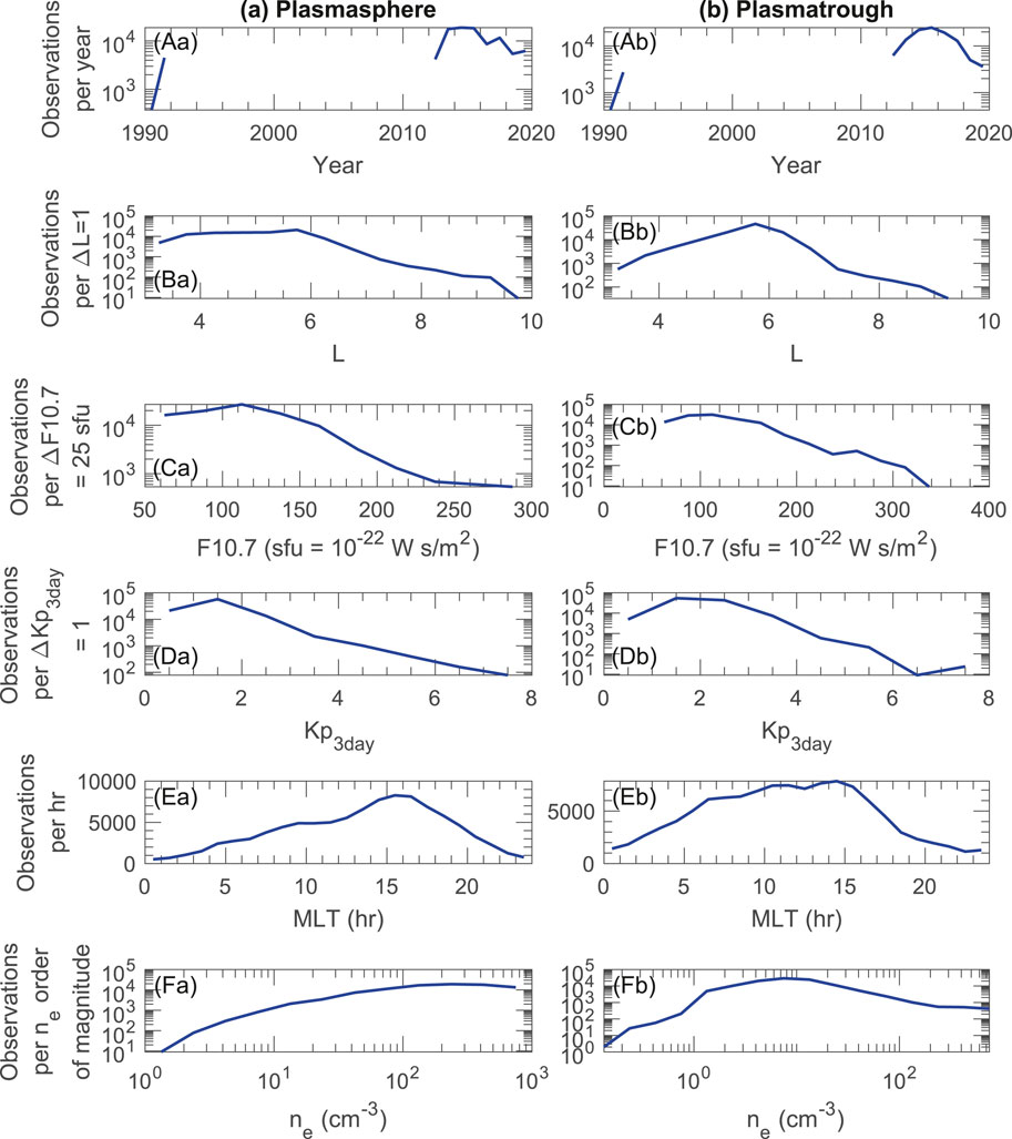
Figure 1 shows the occurrence distributions of our plasmasphere and plasmatrough data sets with respect to a number of parameters. Our figures will follow the convention that uppercase letters are used to indicate rows of panels, lowercase letters are used to indicate columns of panels, and a combination of an uppercase and lowercase letter indicates a specific panel. Thus Figure 1A refers to the upper row of panels, Figure 1a refers to the left column of labels, and Figure 1Aa refers to the upper left panel.

As expected, a larger fraction of the observations is at low $L$ and high $n_{\text{e}}$ for the plasmasphere than for the plasmatrough (Figures 1B, F). Most of the plasmasphere observations are within $L=6$ and the plasmatrough observations peak at about $L=5.75$ (Figure 1B). The best representation of observations is for values of F10.7 less than 150 sfu (Figure 1C) and for values of ${\text{Kp}}_{3\text{day}}$ less than 2.5 (Figure 1D). There are more observations in the plasmatrough with higher Kp values (Figure 1D) because high Kp causes the plasmapause to be at lower $L$ (see Section 3.5), yielding a greater number of observations in the plasmatrough. Observations are more likely on the dayside ($6\mathrm{h}<\mathrm{M}\mathrm{L}\mathrm{T}<18\mathrm{h}$, Figure 1E), but the distributions with respect to MLT in Figure 1 are shown with a linear scale, so there are a significant number of observations on the nightside.

2.4 Training and test data

For three sets of data, plasmasphere, plasmatrough, and both plasmasphere and plasmatrough, we separated the data into training and test data using the following procedure. The data were first put in chronological order. Then the data were divided into 100 sections, each with an equal number of data points (but not necessarily an equal amount of time). Within each of those 100 sections, the middle 12% of data was split off into test data. The purpose of this procedure was to have a similar overall distribution of conditions (by using training and test data with the same set of 100 sections), but to not have training and test data that were practically equivalent because they were measured at almost the same times. This procedure should result in a better test of the formulas than if the test data were randomly chosen (Denton et al., 2022). The median time span of the 12% test data segments was 1.9 days for the plasmasphere, 1.8 days for the plasmatrough, and 2.2 days for plasmasphere and plasmatrough data.

2.5 Turingbot

Turingbot (Ruggiero, 2024) is an artificial intelligence program that discovers mathematical equations. More specifically, it is a symbolic regression program that uses simulated annealing to search the space of possible equations in order to find the equations that best fit a set of data. For each level of complexity, it finds the equation that best fits the data using a certain error metric; we used the root mean squared error (RMSE). Our TuringBot runs sampled billions of different formulas, and the best fitting model for each level of complexity was determined using cross validation with five groups of randomly sorted data taken from the training data set described in Section 2.4.

The TuringBot complexity is described by the mathematical operations, a cost of 1 for introducing a variable or constant or calculating a sum, difference or product, a cost of two for division, and a cost of 4 for all other operations including logarithms and power laws. For instance, the formula $x/y+3z$, would have a complexity of 8, 1 for each of the 3 variables, one for the constant “3”, two for the division, 1 for the multiplication, and 1 for the sum. We only retained formulas if they have a lower cross validation RMSE using the training data and a lower RMSE for the test data than for all of the simpler formulas.

3 Results

3.1 Histograms of measurements

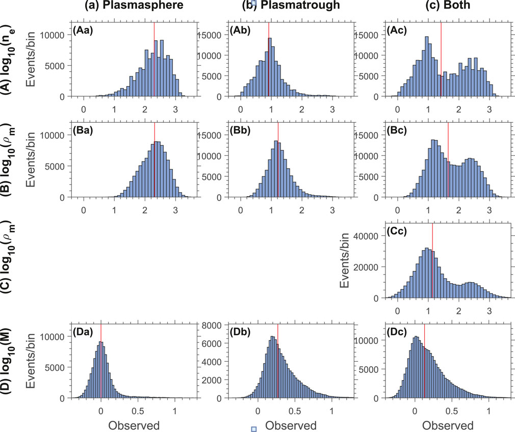
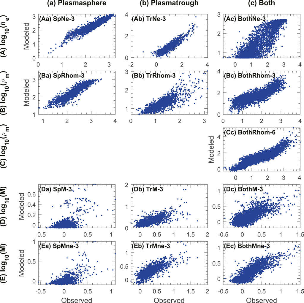
Figure 2 shows histograms of values of the base 10 logarithm of the electron density, $n_{\text{e}}$, the mass density, ${\rho }_{\text{m}}$, and the average ion mass, $M$. As expected, $n_{\text{e}}$ and ${\rho }_{\text{m}}$ values are larger in the plasmasphere than in the plasmatrough (comparing Figures 2Aa, 2Ba to Figures 2 Ab and 2Bb). Figures 2Ac, 2Bc, for both plasmasphere and plasmatrough data, show a double peaked distribution of densities with the lower densities mostly from plasmatrough measurements, and the higher densities mostly from plasmasphere measurements. The peaks for $n_{\text{e}}$ in Figure 2Ac are better separated than the peaks for ${\rho }_{\text{m}}$ in Figure 2Bc, probably because the plasmasphere and plasmatrough data was separated based on values of $n_{\text{e}}$, and also because there is often not as large a difference between plasmasphere and plasmatrough values of ${\rho }_{\text{m}}$ as there is for $n_{\text{e}}$ (Takahashi et al., 2008).

Figure 2

Figure 2. Histograms of base 10 logarithm of values of electron density, mass density, and average ion mass (A) ${\log }_{10}(n_{\text{e}})$ (B, C) ${\log }_{10}({\rho }_{\text{m}})$, and (D) ${\log }_{10}(M)$ (where $M={\rho }_{\text{m}}/n_{\text{e}}$) for (A) plasmasphere, (B) plasmatrough, and (C) both plasmasphere and plasmatrough. Panel Cc is similar to panel Bc, except that a larger database is used for panel Cc, as described in Section 2.1. The red vertical lines are at median values.

Figure 2Cc shows ${\rho }_{\text{m}}$ using the larger database of mass density values that includes GOES, AMPTE CCE, Geotail, and THEMIS, as well as CRRES and the Van Allen Probes (Section 2.1). The distribution in Figure 2Cc is similar to that in Figure 2Bc except that there is a larger number of low ${\rho }_{\text{m}}$ values, owing to the fact that the added spacecraft mostly sampled positions in the plasmatrough.

Figure 2D shows histograms of ${\log }_{10}(M)$. In principle, the minimum value of $M$ should be 1 amu, corresponding to ${\log }_{10}(M)=0$, for an H+/e plasma composed entirely of protons and electrons. But some values of ${\log }_{10}(M)$ are less than zero, corresponding to $M$ less than unity, because of the experimental errors in the determination of ${\rho }_{\text{m}}$ and $n_{\text{e}}$.

Figure 2D shows that the $M$ values are higher for the plasmatrough (Figure 2Db) than for the plasmasphere (Figure 2Da).

Aside from a very small amount of data in a high $M$ tail, the values of ${\log }_{10}(M)$ for the plasmasphere in Figure 2Da are remarkably clustered around a value of zero, which would correspond to $M=1$. Indeed, the median value of ${\log }_{10}(M)$ in the plasmasphere was $-6.4\times 10^{-4}$, corresponding to $M=0.9985$, almost exactly equal to unity. A value of $M=1$ would mean that plasma ions are all H+.

The average value of $M=10^{{\log }_{10}(M)}$ in the plasmasphere was higher, 1.158, corresponding to $M=1.045$. Assuming zero O+ in the plasmasphere, that would correspond to an He+ concentration, ${\eta }_{\text{He}+}\equiv n_{\text{He}+}/n_{\text{e}}$, of 5.2% using

$M\equiv {\rho }_{\text{m}}/n_{\text{e}}=1\left(1-{\eta }_{\text{He}+}\right)+4\left({\eta }_{\text{He}+}\right)=1+3{\eta }_{\text{He}+}(6)$

for an H+/He+/e plasma (Averaging $(M-1)/3$ would lead to the same result). Therefore, our results suggest that the He+ concentration is very low in the plasmasphere, lower than people often assume (10%). If there were a significant amount of O+, with its heavier mass, in the plasmasphere, the concentration of He+ and O+ would have to be even smaller. For instance, an average value of $M=1.158$ would correspond to an O+ concentration of only 1% for an H+/O+/e plasma.

3.2 Models for electron density

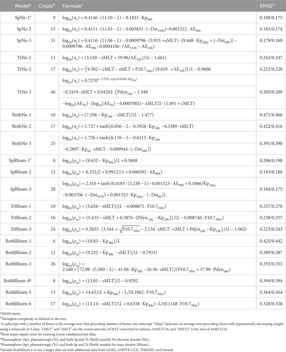
Table 1 shows our models for electron density and mass density. The names of the models in the first column of Table 1 are composed of three parts, “Sp”, “Tr”, or “Both” for plasmasphere, plasmatrough, or both plasmasphere and plasmatrough, “Ne” or “Rhom” for electron density or mass density, and 1, 2, or 3. We limited the number of models for each condition to three, although TuringBot typically yielded more models. Models with the number 1 are the simplest, with two or at most three parameters. Models 1 and 2 are usually easy to interpret, whereas models 3 are sometimes difficult to interpret. The root mean squared error (RMSE) is smaller for the more complex equations.

Table 1

Table 1. Models for electron density and mass density.

By examining the parameters that occur in the simplest models, we can determine which parameters have the strongest effect (Denton et al., 2022). Usually the most important parameters will appear in the models numbered 1. But we can get more information from the full list of models (not shown).

For instance, considering first the models for electron density (Ne), and both plasmasphere and plasmatrough data (Both) in Table 1, the BothNe-1 model suggests that $L$ and ${\text{Kp}}_{24\text{h}}$ are the most important parameters. But simpler models not listed depend only on $L$, so $L$ is the most important parameter. In order of greatest to least importance, $n_{\text{e}}$ decreases with increasing $L$, decreases with increasing geomagnetic activity as indicated by Kp averaged over 24 h, maximizes at sMLT = −1, corresponding to a peak at MLT = 18 h (dusk local time), especially for large values of Kp averaged over 6 h, and decreases with respect to more negative Dst averaged over 48 h.

In our descriptions below, we will for simplicity refer to averages of parameters over a certain amount of time as just that parameter. For instance, instead of saying ${\text{Kp}}_{48\text{h}}$, we will just say Kp. For the exact values preferred by the models, see Tables 1, 2. We also write the models in terms of -Dst, because more negative Dst corresponds to more geomagnetically active conditions.

Table 2

Table 2. Models for average ion mass, M.

Considering the models for electron density in the plasmasphere (SpNe) in Table 1, $L$ is again the most important parameter. The Kp parameter appears next in model SpNe-1, but is then replaced by -Dst and AE in model SpNe-2. So some combination of these parameters is also important; $n_{\text{e}}$ decreases with respect to Kp, AE, and -Dst. Finally, the dependence on MLT is much weaker in the plasmasphere; sMLT only appears in the most complicated model (SpNe-3). In that model, $n_{\text{e}}$ is again maximized at sMLT = −1, corresponding to MLT = 18 h (dusk local time).

The MLT dependence is much stronger in the plasmatrough. Again the most important dependence is that $n_{\text{e}}$ decreases with increasing $L$, but the next strongest dependence is maximum value at sMLT = −1, yielding again a peak in density at dusk local time. In the next, more accurate model (TrNe-2), $n_{\text{e}}$ has maximum value at maximum -(sMLT + cMLT), yielding a peak at MLT = 15 h (afternoon local time) (A more complex model might have different coefficients for sMLT and cMLT). Additionally $n_{\text{e}}$ decreases with respect to increasing AE. Model TrNe-2 shows that $n_{\text{e}}$ increases with respect to increasing F${10.7}_{3\text{day}}$, but that dependence is replaced by a dependence on Kp and Pdyn in the TrNe-3 model, for which $n_{\text{e}}$ decreases with increasing Kp and increases with increasing Pdyn.

So, in summary, $n_{\text{e}}$ decreases with respect to increasing $L$, and decreases with respect to increasing geomagnetic activity as indicated by AE, Kp, and -Dst in all regions. There is a peak at afternoon to dusk local time, much stronger for the plasmatrough. The electron density increases with respect to increasing F10.7 and Pdyn in the plasmatrough.

We have already noted that $n_{\text{e}}$ is larger in the plasmasphere than in the plasmatrough (Figure 2A), consistent with how these regions were defined. Figure 3A shows scatterplots of model values of ${\log }_{10}(n_{\text{e}})$ versus observed values for the most complicated models of Table 1, using only the test data that was not used as input to the models (the most stringent test). The models do a much better job for the plasmasphere (Figure 3Aa) or plasmatrough (Figure 3Ab) than for the combined data set (Figure 3Ac). This is also evident from the RMSE values in Table 1, 0.169 and 0.209 for test data using the SpNe-3 and TrNe-3 models, respectively, but 0.3904 for the BothNe-3 model. This is evidently because of the large variation of density at intermediate values of ${\log }_{10}(n_{\text{e}})$, which corresponds to positions within the plasmapause (Figure 3Ac).

Figure 3

Figure 3. Scatter plots of base 10 logarithm of model values of electron density, mass density, and average ion mass versus base 10 logarithm of observed values for the test data. For (A) ${\log }_{10}(n_{\text{e}})$, (B, C) ${\log }_{10}({\rho }_{\text{m}})$, and (D, E) ${\log }_{10}(M)$, and for (A) plasmasphere, (B) plasmatrough, and (C) both plasmasphere and plasmatrough, scatterplots of model values versus observed values. Only one out of seven data points are plotted. The specific models used are indicated in the panel labels, for instance, model SpNe-3 in panel Aa. The larger database is used for panel Cc, as described in Section 2.1. The models in Figure 3E allow ${\log }_{10}(n_{\text{e}})$ as an input parameter, whereas those in Figure 3D do not.

3.3 Models for mass density

Now we turn to models for mass density in Table 1. Looking first at the models using both plasmasphere and plasmatrough data and based on the bigger database described in Section 2.1 (BothRhom-4–6), in order of greatest to least importance, the dependencies are decreasing ${\rho }_{\text{m}}$ with respect to increasing $L$, maximum ${\rho }_{\text{m}}$ at sMLT = −1, corresponding to MLT = 18 h, decreasing ${\rho }_{\text{m}}$ with respect to increasing Kp, and increasing ${\rho }_{\text{m}}$ with respect to F10.7. The $L$, MLT, and Kp dependencies are the same as occurred for $n_{\text{e}}$.

These dependencies also occur in the plasmasphere (models SpRhom-1–3 in Table 1), except that the dependence on F10.7 does not appear (There may be some dependence at smaller $L$, but we are only using data with $L\ge 3.25$.). In addition, ${\rho }_{\text{m}}$ decreases with increasing AE (model SpRhom-2), like $n_{\text{e}}$ did. The Dst dependence is somewhat complicated. Increasing Kp by itself or more negative Dst by itself lead to decreasing ${\rho }_{\text{m}}$, but there is a positive nonlinear term in model SpRhom-3 with the product of ${\mathrm{K}\mathrm{p}}_{3\text{day}}$ and $(-{\mathrm{D}\mathrm{s}\mathrm{t}}_{192\text{h}})$.

In the plasmatrough, we find the same dependencies as occurred for both plasmasphere and plasmatrough data plus an additional positive correlation of ${\rho }_{\text{m}}$ with Pdyn. For the plasmatrough, the Pdyn and F10.7 dependence may be stronger than that of Kp, since Pdyn and F10.7 occur in a slightly simpler formula than one containing Kp. For the plasmatrough data, in order from greatest to least importance, the dependencies are decreasing ${\rho }_{\text{m}}$ with respect to $L$, ${\rho }_{\text{m}}$ maximized at sMLT = −1, corresponding to MLT = 18 h (dusk local time), increasing ${\rho }_{\text{m}}$ with respect to increasing Pdyn and F10.7, and decreasing ${\rho }_{\text{m}}$ with respect to Kp.

Figures 3B, C show scatterplots of values of ${\log }_{10}({\rho }_{\text{m}})$ using the most complicated model for each case versus observations of $\log ({\rho }_{\text{m}})$.

As was the case for $n_{\text{e}}$, the RMSE is smaller for the plasmasphere or plasmatrough data sets than for a data set combining plasmasphere and plasmatrough data. For instance, using the test data and the most complicated models, the RMSE is 0.175 and 0.243 for the plasmasphere and plasmatrough, respectively, whereas for both plasmasphere and plasmatrough data together, it is 0.353 for model BothRhom-3 using only the CRRES and Van Allen Probes data, or 0.3284 for model BothRhom-6 using the larger database with more spacecraft.

It might seem strange that there is a larger error for both plasmasphere and plasmatrough data using the larger database, because the smaller database corresponds to a more narrow range of $L$. Normally one would think that a more precise model would be possible for a narrower range of conditions. But the smaller database uses the CRRES and Van Allen Probes data that have a larger number of densities within the plasmapause compared to the other spacecraft used in the larger database.

3.4 Models for average ion mass

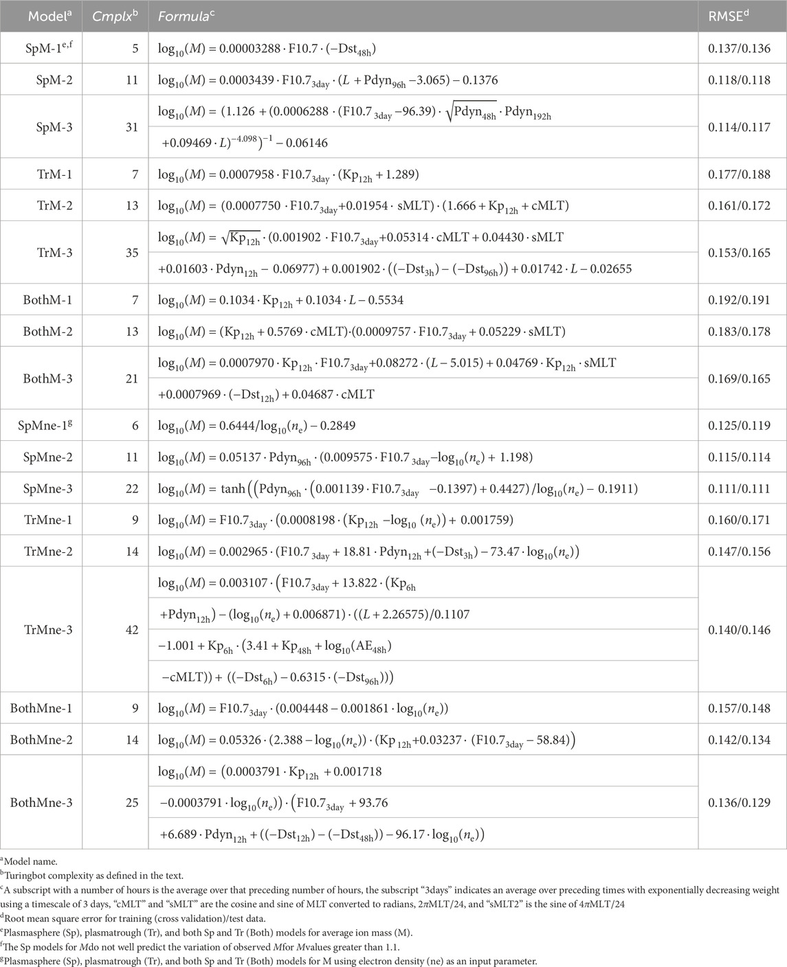
The models in Table 2 show the dependence of $M\equiv {\rho }_{\text{m}}/n_{\text{e}}$ on various parameters. The model names now include “M” or “Mne”. A model with “Mne” in the model name allows $n_{\text{e}}$ as an input parameter, whereas models with just “M” in the model name do not. So models SpM-1 through BothM-3 in Table 2 do not include $n_{\text{e}}$ as an input parameter, whereas models SpMne-1 through BothMne-3 do. The latter models are included for spacecraft observations that measure $n_{\text{e}}$. Using $n_{\text{e}}$ as an input parameter allows for a better dependence on $n_{\text{e}}$ than just breaking up the data into plasmasphere and plasmatrough data. On the other hand, those models may be more influenced by the errors in $n_{\text{e}}$ since $M$ is defined using $n_{\text{e}}$.

The mass density depends more strongly on F10.7 than does the electron density, at least in the plasmatrough, so it is not surprising that $M$ increases with increasing F10.7. This is in agreement with results by Takahashi et al. (2010) and Denton et al. (2011), who showed that larger $M$ correlates with larger F10.7, which occurs at solar maximum. But most of the other parameters cause similar changes in both ${\rho }_{\text{m}}$ and $n_{\text{e}}$, so the dependence of $M$ on these parameters will depend on whether the ${\rho }_{\text{m}}$ or $n_{\text{e}}$ dependence is stronger.

Some interesting dependencies occur for the plasmasphere data. For instance, model SpM-1 indicates that the combination of F10.7 and (-Dst) leads to increasing $M$, and model SpM-2 suggests that the combination of increasing F10.7 multiplied by $L$ and/or Pdyn leads to increasing $M$. Not surprisingly, considering the definition of $M\equiv {\rho }_{\text{m}}/n_{\text{e}}$, model SpMne-1 shows that $M$ increases for decreasing $n_{\text{e}}$.

The RMSE of the models for $M$ in the plasmasphere is small, 0.117 using the test data for model SpM-3, or 0.111 using the test data for model SpMne-3. But the reason that the RMSE is so small for the plasmasphere is because most of the data points are clustered around ${\log }_{10}(M)=0$, or $M=1$, as discussed in Section 3.1. Removing the data points with model values of ${\log }_{10}(M)$ less than about 0.1, there is a very poor correlation between the remaining observed and model values in Figure 3Da, 3Ea. Consequently, the formulas for $M$ in the plasmasphere may have limited usefulness.

There is a better correlation between observed and model values of $M$ in the plasmatrough, as shown in Figure 3Db, 3Eb. In the plasmatrough, considering the models without $n_{\text{e}}$ as an input parameter (TrM), the most important dependences are that $M$ increases with increasing F10.7, and that $M$ increases with increasing Kp. The next most important dependence is on MLT, with a positive sMLT dependence (peak at dawn local time) first appearing. Considering all of the models, there is a peak in $M$ between MLT = 0 h and 6 h (pre-dawn local time). Considering that $n_{\text{e}}$ and ${\rho }_{\text{m}}$ both have maximum value at afternoon to dusk local time, that means that the plasmatrough plasma at dawn is low density plasma made up of relatively heavier ions than those at dusk local time.

In addition, $M$ in the plasmatrough increases with respect to increasing Pdyn and $L$, and with respect to increasing negative Dst on a short timescale, subtracting off an average over a larger amount of time (e.g. (-Dst3h)-(-${\text{Dst}}_{96\text{h}}$) dependence in model TrM-3).

Seeing as there was almost no variation of $M$ in the plasmasphere, it’s not surprising that we see the same dependencies for $M$ using both plasmasphere and plasmatrough data as those for $M$ in the plasmatrough. There are some subtleties. For instance, model BothM-3 indicates that for ${\text{Kp}}_{12\text{h}}$ greater than about unity, the peak in $M$ will be closer to MLT = 6 h, whereas for ${\text{Kp}}_{12\text{h}}$ less than about unity, the peak in $M$ will be closer to MLT = 0 h.

3.5 Example density dependencies

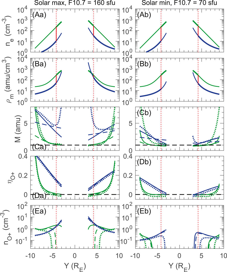
As an illustration of the use of our formulas, we show in Figure 4a the SM Y dependence at SM X and Z equal to zero (dawn to dusk cut across the magnetic equator) of $n_{\text{e}}$, ${\rho }_{\text{m}}$, $M$, the O+ concentration, ${\eta }_{\text{O}+}\equiv n_{\text{O}+}/n_{\text{e}}$, and the O+ density, $n_{\text{O}+}$, for active conditions with Kp equal to 3, and at solar maximum with F10.7 equal to 160 sfu. These values were chosen to lead to large $M$ based on models TrM-1 and BothM-3. Other parameter values were Dst equal to −25 nT, AE equal to 250 nT, and Pdyn equal to 2.5 nPa. These last three parameter values were median values for the times in our database at which F10.7 and Kp were large. For simplicity, we use the same values for all averages.

Figure 4

Figure 4. Example of density dependence based on plasmasphere and plasmatrough models for active conditions. (A) Electron density, $n_{\text{e}}$, (B) mass density, ${\rho }_{\text{m}}$, (C) average ion mass, $M$, (D) O+ concentration, ${\eta }_{\text{O}+}$, and (E) O+ density, $n_{\text{O}+}$, at (A) solar maximum, and (B) solar minimum, for plasmasphere (green curves) and plasmatrough (blue curves). The most complicated models from Tables 1, 2 were used in each case. The curves for $M$ in row C are found from models using $n_{\text{e}}$ (solid curves), from models for $M$ not using $n_{\text{e}}$ as input (dashed curves), and by dividing model values for ${\rho }_{\text{m}}$ by model values of $n_{\text{e}}$ (dotted curves). The curves for ${\eta }_{\text{O}+}$ and $n_{\text{O}+}$ in rows (D, E) are found from the model for $M$ using $n_{\text{e}}$ as input [solid curves in row (C)] and assume zero He+ (solid curves), the Craven et al. (1997) model (dashed curves), and 10% light ion density (dotted curves). Tne vertical dashed lines are the plasmapause position based on a model by Carpenter and Anderson (1992).

Curves are shown in Figure 4 for geocentric radius $R=|Y|\ge 3$ $R_{\text{E}}$, slightly lower than our restriction on the data, $R\ge 3.25$ $R_{\text{E}}$.

Figure 4Aa shows $n_{\text{e}}$ from models SpNe-3 and TrNe-3. The plasmasphere $n_{\text{e}}$ (green curves) decreases linearly with respect to $R$ ($=L$ here at the magnetic equator), as indicated by model SpNe-3 in Table 1. The plasmatrough $n_{\text{e}}$ values (blue curves) are lower than the plasmasphere values. Both plasmasphere and plasmatrough densities are larger at positive Y (dusk local time) than at negative Y (dawn local time).

The vertical dashed red lines in Figure 4 are at plus or minus the $L$ value of the plasmapause of Carpenter and Anderson (1992) (their Equation 7),

$L_{\text{pp}}=5.6-0.46{\mathrm{K}\mathrm{p}}_{\text{max}},(7)$

where their ${\text{Kp}}_{\text{max}}$ is the maximum value in the preceding 24 h with some modification (see Carpenter and Anderson, 1992). We have used ${\text{Kp}}_{\text{max}}$ = 3 for simplicity. If the vertical dashed red lines delineate the boundary of the plasmasphere and plasmatrough, the green curves would be valid at $R<L_{\text{pp}}$ (bolder sections of green curves), the blue curves would be valid at $R>L_{\text{pp}}$ (bolder sections of blue curves), and the plasmapause would join the inner green curve to the outer blue curve roughly along the vertical red line segments.

Figure 4Ba shows ${\rho }_{\text{m}}$ from models SpRhom-3 and TrRhom-3. Note that the values of ${\rho }_{\text{m}}$ (in amu/${\mathrm{c}\mathrm{m}}^3$) are close to those of $n_{\text{e}}$ (in ${\text{cm}}^{-3}$) within the plasmapause at $R=L_{\text{pp}}$, but the values of ${\rho }_{\text{m}}$ become significantly larger than those of $n_{\text{e}}$ outside of the plasmapause at $R=L_{\text{pp}}$.

The solid curves in Figure 4Ca show $M$ from models SpMne-3 and TrMne-3 in Table 2, using $n_{\text{e}}$ as an input parameter. Where model SpMne-3 predicted a value of $M$ less than unity $(R\le 2.5R_{\text{E}})$, $M$ was set equal to unity (horizontal dashed black line). In the plasmasphere (green curves), $M$ is equal to or very close to 1 within the vertical dashed red lines, but is increasing with respect to $R$. While this trend may very well be representative on average, the large values of $M$ at $R=9$ $E_{\text{E}}$ could be unrealistic. Very few of our data were at this larger value of $L$ (Figure 1B), and as discussed in Sections 3.1, 3.4, the correlation between observed and model values of plasmasphere $M$ was very poor for values significantly greater than unity (This comment would not matter if the plasmapause curves are only relevant inside the vertical dashed red lines, but if there were a plasmaspheric plume with large density extending beyond those vertical dashed lines, the large $M$ values of the green curves outside of the vertical dashed red lines in Figure 4Ca might be misleading).

The solid curves in Figure 4Ca are used to derive the curves shown in Figures 4D, E. But we also show in Figure 4C values of $M$ from models SpM-3 and TrM-3, which did not use $n_{\text{e}}$ as an input parameter (dashed curves in Figure 4C) and $M$ calculated by dividing values of ${\rho }_{\text{m}}$ from models SpRhom-3 and TrRhom-3 in Figure 4B by values of $n_{\text{e}}$ from models SpNe-3 and TrNe-3 in Figure 4A (dotted curves in Figure 4C).

The curves in Figure 4C based on different methods (solid, dashed, or dotted) differ. But except near $R=9R_{\text{E}}$, the plasmatrough values of $M$ (blue curves) are significantly greater than those in the plasmasphere (green curves). But the plasmatrough $M$ values also increase with respect to $R$. For both plasmasphere and plasmatrough, the $M$ values are larger on the dawn side $(Y<0)$.

Using Equation 3 to get the O+ density, we tried modeling the O+ concentration and O+ density from individual data points, but the inferred O+ values were too noisy, so we decided to use our models for $n_{\text{e}}$ and $M$ with assumptions for the He+ concentration.

Figure 4Da shows the O+ concentration, ${\eta }_{\text{O}+}$, using Equation 3 with model SpNe-3 or TrNe-3 from Table 1 and model SpMne-3 or TrMne-3 from Table 2 (using $n_{\text{e}}$ as input; solid curves in Figure 4C) for three different models of He+ concentration, zero He+ or ${ϵ}_{\text{He}}=0$ in Equation 2 (solid curves), the Craven et al. (1997) model (dashed curves), and ${ϵ}_{\text{He}}=0.1$ (dotted curves). The Craven et al. (1997) model [better described by Del Corpo et al. (2022)] for the He+ to H+ density ratio, $R_{\text{He}}$, is

${\log }_{10}\left(R_{\text{He}}\right)=-1.541-0.176R+8.557\times 10^{-3}P-1.458\times 10^{-5}{P}^2,(8)$

where $P$ is the average of the instantaneous F10.7 and a time centered (strangely, considering causality) average of F10.7 over 81 days, and ${ϵ}_{\text{He}}=R_{\text{He}}/(1+R_{\text{He}})$. The Craven et al. (1997) model leads to $R_{\text{He}}$ generally greater than 0.1 only at low $R\le 2$ $R_{\text{E}}$, and $R_{\text{He}}$ generally less than 0.1 for $R\ge 4$ $R_{\text{E}}$ (see Craven et al.‘s Figure 2).

Where $M$ is much larger than unity in Figure 4Ca, the model for He+ doesn’t make much difference to the O+ concentration in Figure 4Da, but where $M$ approaches unity, so that the He+ has a significant impact on $M$, the model for He+ does strongly affect the O+ concentration. Since we have required $M\ge 1$, ${\eta }_{\text{O}+}$ will never be less than zero for ${ϵ}_{\text{He}}=0$ (solid curves in Figure 4Da). But if $M$ is close to or equal to unity, and ${ϵ}_{\text{He}}$ is not zero, Equation 4 can yield ${\eta }_{\text{O}+}<0$, which means that our models for $M$ are inconsistent with the assumed concentration of He+.

The value of ${\eta }_{\text{O}+}$ is always greater than zero in the plasmatrough for $R\ge 3$ $R_{\text{E}}$ (blue curves in Figure 4Da). But for the plasmasphere with ${ϵ}_{\text{He}}=0$, ${\eta }_{\text{O}+}$ becomes zero for $-2.5R_{\text{E}}<Y<2.8R_{\text{E}}$ (solid green curves in Figure 4Da). Using the Craven et al. (1997) model (dashed green curves), ${\eta }_{\text{O}+}$ becomes less than zero for $-4.3R_{\text{E}}<Y<4.5R_{\text{E}}$, and using ${ϵ}_{\text{He}}=0.1$ (dotted green curves), ${\eta }_{\text{O}+}$ becomes less than zero for $-5.3R_{\text{E}}<Y<5.5R_{\text{E}}$. The locations where ${\eta }_{\text{O}+}\le 0$ can also be identified from Figure 4Ea, at the locations where curves for $n_{\text{O}+}$ plunge toward zero (and would become negative plotting with a linear scale).

If we consider the vertical red dashed lines to separate the plasmasphere and plasmatrough (as discussed above), then there would be a region of nonzero $n_{\text{O}+}$ within the plasmasphere only if ${ϵ}_{\text{He}}$ is close to zero (solid green curves in Figure 4Da). In that case, there would be a peak in $n_{\text{O}+}$ within the plasmasphere on the dawn side at about $Y=-3.9R_{\text{E}}$. On the dusk side, the peak in $n_{\text{O}+}$ would be on the plasmatrough side of the plasmapause, but there would be some O+ within the plasmasphere. On either side, $n_{\text{O}+}$ would decrease with respect to $R$ in the plasmatrough, and would decrease steeply at $R<3R_{\text{E}}$ in the plasmasphere. But, if there would be as much He+ as is required by the Craven et al. (1997) model (dashed green curves in Figure 4Da) or ${ϵ}_{\text{He}}=0.1$ (dotted green curves in Figure 4Da), there would be no O+ within the plasmasphere, since the dashed and dotted green curves in Figure 4Da go below zero within the plasmasphere. In that case, the O+ would be entirely outside the plasmasphere within the plasmatrough.

The possibility that our models might not lead to O+ within the plasmasphere for the models with a greater amount of He+ is not surprising considering that our median $M$ value for the plasmasphere was slightly less than unity and that the average $M$ value for the plasmasphere was consistent with a He+ concentration of only 5.2%.

Although ${\eta }_{\text{O}+}$ is greater on the dawn side $(Y<0)$ than on the dusk side $(Y>0)$ in Figure 4Da, $n_{\text{O}+}$ in Figure 4Ea is in most cases greater on the dusk side $(Y>0)$, especially in the plasmatrough (blue curves in Figure 4Ea). This can occur because of the greater density on the dusk side (Figures 4Aa, 4Ba). These results are consistent with those of Denton et al. (2014b), who examined the local time dependence of electron and mass density at geostationary orbit.

Figure 4b uses the same geomagnetic conditions as Figure 4a, except that F10.7 has been decreased to 70 sfu, a value characteristic of solar minimum. First of all, note that the curves in Figure 4Ab are identical to those in Figure 4Aa because our models for $n_{\text{e}}$ in both the plasmasphere and the plasmatrough do not depend on F10.7.

The values of $M$ at solar minimum in Figure 4Cb, however, are significantly lower than those in Figure 4Ca. Our models yield much more O+ at solar maximum than at solar minimum (Takahashi et al., 2010; Denton et al., 2011). For these (very active) conditions, there is no region for which ${\eta }_{\text{O}+}>0$ within the plasmasphere at $R$ within the vertical red dashed lines. That means that based on Figure 4b, there is no O+ in the plasmasphere, and a smaller density of O+ (compared to that at solar maximum, Figure 4Ea) peaks just outside of the plasmapause and decreases at increasing $R$ (Figure 4Eb). Whether or not $n_{\text{O}+}$ is larger in the dusk or dawn plasmatrough depends on the value of $R$ and the He+ concentration.

Figure 5 has the same format as Figure 4, except that geomagnetically quiet conditions are assumed, with Kp = 0.5, Dst = 0, Pdyn = 2.5 nT, and AE = 30 nT. Although the instantaneous values of these parameters may have lower values, the values that we used are very low values for the averages used in the formulas. $L_{\text{pp}}$ was set equal to 5.4 $R_{\text{E}}$ using Equation 8.

Figure 5

Figure 5. Example of density dependence based on plasmasphere and plasmatrough models for quiet conditions, using the same format as Figure 4. Note that the dotted curve in panel Eb is everywhere negative for $Y>0$. The dotted curves in rows (A, B) are found from accumulating observed values onto a grid, as described in the text.

Figure 5E suggests that there is no O+ within the plasmasphere for very quiet conditions (green curves with $n_{\text{O}+}>0$ inside the vertical red dashed lines) except just inside the plasmapause for solar max if there is no He+ (solid green curve in Figure 5Ea). Based on Figure 5E, there is some O+ in the plasmatrough for very quiet conditions, but Figure 5Eb suggests that for very quiet conditions at solar minimum, the O+ density is very low, and extremely low (or nonexistent at dusk) if ${ϵ}_{\text{He}+}=$ 10% (Figure 5Eb).

4 Discussion

4.1 General characteristics of models

We have derived a number of empirical models that should be useful for describing the magnetospheric plasma, including models for the electron density, $n_{\text{e}}$, and mass density, ${\rho }_{\text{m}}$, in Table 1, and models for the average ion mass, $M$, in Table 2. Models of varying complexity include dependence on $L$, MLT, geomagnetic activity as indicated by Kp, Dst, and AE, and phase of the solar cycle as specified by F10.7. Formulas are included for plasmasphere, plasmatrough, and for both plasmasphere and plasmatrough, and three models of varying complexity are included for each condition. Formulas for $M$ in Table 2 include formulas with or without $n_{\text{e}}$ as an input parameter.

Because $M$ is ${\rho }_{\text{m}}$ divided by $n_{\text{e}}$, the dependence of $M$ on various parameters will depend on whether ${\rho }_{\text{m}}$ or $n_{\text{e}}$ depends more strongly on that parameter. Both ${\rho }_{\text{m}}$ and $n_{\text{e}}$ increase with respect to increasing F10.7 and Pdyn, but these dependencies are stronger for ${\rho }_{\text{m}}$ than for $n_{\text{e}}$, so that $M$ increases with respect to both increasing F10.7 and Pdyn. The strongest dependence of $M$ is on F10.7.

Both ${\rho }_{\text{m}}$ and $n_{\text{e}}$ decrease with respect to $L$, have a maximum at afternoon to dusk local time, and decrease with respect to geomagnetic activity, as specified by parameters like Kp, AE, and -Dst. But these dependencies are stronger for $n_{\text{e}}$ than for ${\rho }_{\text{m}}$ so that $M$ has the opposite dependencies, increasing with respect to increasing $L$, having a maximum at midnight to dawn local time, and increasing with respect to increasing geomagnetic activity as specified by Kp, AE, and -Dst.

In our models, parameters such as Kp and F10.7 appear as quantities averaged over various amounts of time. For the exact dependencies, see Tables 1, 2.

For the development of the electron density models in Table 1, we forgot to adjust the electron density to a value at the magnetic equator. This neglect is consistent with an assumption that $n_{\text{e}}$ is constant along magnetic field lines. But ideally, we would multiply the plasmasphere electron density by something like $R/L$ and the plasmatrough electron density by something like ${(R/L)}^2$ to account for observed field line dependence (Denton et al., 2004; 2006) (We did make that adjustment in Section 4.2 below). However, this correction was not a serious problem because the spacecraft that we used had low inclination orbits; when we evaluated the logarithmic RMS errors for our electron density models including this correction for the observed densities, the errors only changed by less than 5% (And this issue doesn’t affect our model results for ${\rho }_{\text{m}}$ or $M$).

4.2 Comparison with other models

Here we make a limited comparison of our models to other empirical models using data sets that were not used in our study, as described above.

Del Corpo et al. (2020) developed a model for plasmatrough mass density using ground magnetometers. They presented evidence that for $L>3.5$ their data was consistent with plasmatrough densities if Kp had been greater than 5 during the past 24 h. So they required that ${\text{Kp}}_{\text{max}24\text{h}}$ be greater than 5, where ${\text{Kp}}_{\text{max}24\text{h}}$ is the maximum value of Kp during the previous 24 h. They limited their study to $L>3.8$ and also to 6 h $<\mathrm{M}\mathrm{L}\mathrm{T}<$ 18 h. With these limitations, they found

${\rho }_{\text{m}}=\left(30+17.4\left(\mathrm{M}\mathrm{L}\mathrm{T}-6\right)\right){\left(\frac{L}{4}\right)}^{-3.65-0.112\left(\mathrm{M}\mathrm{L}\mathrm{T}-6\right)}\left(\mathrm{a}\mathrm{m}\mathrm{u}/{\mathrm{c}\mathrm{m}}^3\right).(9)$

Using the same restrictions, we tested their model and our models TrRhom-1, TrRho-2, and TrRho-3 in Table 1 using the THEMIS data (Section 2.1), which was not used to develop any of these models. The logarithmic RMSE was 0.318 for Del Corpo’s model (Equation 9), and 0.265, 0.275, and 0.228 for models TrRhom-1, TrRho-2, and TrRho-3, respectively. Therefore our models agree better with the THEMIS data, and the errors for our models for the THEMIS data are similar to those in Table 1, except that the error for model TrRho-2 is somewhat higher than that of TrRho-1. This is remarkable considering that we used Del Corpo’s method to select plasmatrough data, which is very different from the method we used in our study.

The most important dependence of ${\rho }_{\text{m}}$ in the plasmatrough is on the spatial parameters (Section 3.3), and the Del Corpo et al. (2020) model has a more sophisticated spatial dependence than our models. But it lacks the important dependence on F10.7 (model TrRho-1 in Table 1) and other activity dependencies for models TrRho-2 and TrRho-3. TuringBot was able to discover the dependence on these other variables.

Next we compare our plasmasphere models for $n_{\text{e}}$, SpNe-1, SpNe-2, and SpNe-3 in Table 1 to the Carpenter and Anderson (1992) plasmasphere model (SpNe-CA) for $n_{\text{e}}$,

$\begin{array}{ccc}\hfill {\log }_{10}\left(n_{\text{e,CA}}\right)=3.9043-0.3145L+\left[0.15\left(\cos \left(\frac{2\pi \left(d+9\right)}{365}\right)-0.5\cos \left(\frac{4\pi \left(d+9\right)}{365}\right)\right)\right.& \hfill & \hfill \\ \hfill \left.+0.00127\bar{R}-0.0635\right]e^{-\frac{L-2}{1.5}}\left({\mathrm{c}\mathrm{m}}^{-3}\right),& \hfill & \hfill \end{array}(10)$

for $L\ge 2.25$, where $d$ is the day of year number, and $\bar{R}$ is the sunspot number averaged over 13 months, and to the Sheeley et al. (2001) plasmasphere model (SpNe-Sheeley),

${\log }_{10}\left(n_{\text{e,Sheeley}}\right)=1390{\left(\frac{3}{L}\right)}^{4.8}\left({\mathrm{c}\mathrm{m}}^{-3}\right),(11)$

for $3\le L\le 7$ (We might have compared to the more recent Lv et al. (2022) model, that includes dependence on geomagnetic activity, except that they did not list the values of the $a^{\prime }$, $b^{\prime }$, $c^{\prime }$, $a^{″}$, $b^{″}$, and $c^{″}$ parameters that are used in their model. We suspect that the Lv et al. model is overfit (too finely tuned to a particular data set), but cannot show that without knowing the value of these coefficients).

For this comparison, we use our database of electron density measurements from the Imager for Magnetopause-to-Aurora Global Exploration (IMAGE) spacecraft (Denton et al., 2012). IMAGE was a polar orbiting spacecraft; we used only observations at magnetic latitude, MLAT, of 20$°$ or smaller, and adjusted the density to the value at the equator by multiplying by $R/L$ (section 4.1).

We first used all of the IMAGE data for $L\ge 3.25$, and found that the logarithmic RMSE for $n_{\text{e}}$ was 0.2844 for the SpNe-CA model (Equation 10) and 0.244 for the SpNe-Sheeley model (Equation 11), and 0.252, 0.255, and 0.2674 for the SpNe-1, SpNe-2, and SpNe-3 models, respectively. While the errors from our models are slightly lower than that of the SpCA model, these errors are larger than that of the SpNe-Sheeley model and significantly larger than those in Table 1, and the lowest of the errors is for the simplest model.

However, the IMAGE spacecraft, with its apogee of 8.2 Earth radii, had a double peaked distribution with a peak in observations near $L=8$, whereas the plasmasphere observations for our set of data were mostly limited to $L\le 6.5$ (Figure 1Ba). If we limit the IMAGE data to $L\le 6.5$, we get an error of 0.256 for the SpNeCA model, 0.215 for the SpNe-Sheeley model, and 0.179, 0.181, and 0.179 for the SpNe-1, SpNe-2, and SpNe-3 models, respectively. The last numbers are comparable to the errors in Table 1, although for this data set, the simplest SpNe-1 model again performs as well or better than the SpNe-2 and SpNe-3 models (The reduction in error for the limited range of $L$ was greater for our models than for the SpNe-CA model.).

This led us to re-examine the $L$ dependence of our plasmasphere models for the database used in this paper. Limiting the data to $L\ge 7$, we find that the errors of the SpNe-1, SpNe-2, and SpNe-3 models are 0.287, 0.327, and 0.303, respectively. Based on this information, our plasmasphere models for $n_{\text{e}}$ are significantly less accurate beyond $L$ equal to about 6.5. For $3.25\le L\le 6.5$, we find that the logarithmic RMSE is 0.182, 0.176, and 0.172 for the SpNe-1, SpNe-2, and SpNe-3 models, respectively, which are close to the values in Table 1.

Given the restriction to lower $L$, our models probably performed better because they included input variables representing geomagnetic activity, Kp, AE, and Dst, whereas the earlier models did not.

In summary, these tests with other data sets reveal that our models have smaller error than other empirical models, at least if the plasmasphere models are limited to $L\le 6.5$. But although our more complicated models have smaller error than that of the simpler models using our data set, which is dominated by data from the Van Allen Probes, our more complicated models do not always have lower error than the simpler models using other data sets. And our plasmasphere models for electron density become significantly less accurate at $L\ge 7$.

4.3 Plasmasphere models

For the vast majority of our plasmasphere data, $M$ values cluster around $M=1$, consistent with results by Del Corpo et al. (2022). Removing the values with $M\le 1.1$, the correlation between observed and model $M$ values within the plasmasphere is poor (Figures 3Da, 3Ea). Thus for most of our plasmosphere data, $M$ is equal to unity within the error of our measurements. Because of that, our models for $M$ in the plasmasphere may not be very useful. The median value of $M$ for our plasmasphere data was slightly less than unity, implying that the plasmasphere would consist of only H+. The average value was higher, $M=1.045$, consistent with an average He+ concentration of 5.2% assuming no O+.

Most of the data used for the plasmasphere models were from low $L$ (Figure 1Ba), and we would be very cautious about extrapolating our models to large $L$ values within a plasmaspheric plume (characterized by relatively high density). For instance, Figures 4Ca–Da might suggest that the $M$ value and O+ concentration would become very large within a plasmaspheric plume, but results by Takahashi et al. (2008) found $M$ very close to unity within a plasmaspheric plume. Also, whereas our study shows that $M$ becomes close to unity as $L$ approaches 3.25, $M$ should become larger as ionospheric altitudes are approached because of the presence of heavy ions there.

4.4 Study of densities in dawn to dusk cuts

Our examination of densities of electrons and O+ in section 3.5 leads to a number of interesting conclusions. The electron density is not significantly affected by the phase of the solar cycle as indicated by the solar EUV index F10.7, and is larger at dusk local time than at dawn local time. The $M$ value and O+ concentration, ${\eta }_{\text{O}+}$, are higher at dawn local time than at dusk local time, but the O+ density $n_{\text{O}+}$ is comparable at dawn and dusk because of the higher values of $n_{\text{e}}$ at dusk.

It’s impossible to make any firm conclusions about composition in the plasmasphere, because our data was roughly consistent with $M=1$ for a pure H+/e plasma (Section 3.4). But our results suggest that the He+ concentration in the plasmosphere is less than 10%, that there is no O+ within the plasmasphere at solar minimum (Figures 4Eb, 5Eb), and that there is only O+ in the plasmasphere near the plasmapause at solar maximum if the He+ concentration there is very small (Figures 4Ea, 5Ea).

Our models yield some O+ in the plasmatrough, generally decreasing with respect to geocentric radius $R$. For geomagnetically very quiet conditions at solar minimum, the O+ density is extremely low or zero. This last result is an agreement with Denton et al. (2011), who showed that there was no O+ in the magnetosphere at solar minimum for typical conditions, which would be quiet.

Our observations of higher $M$ at dawn local time are consistent with results by Nose et al. (2018) for the “oxygen torus”, but we have shown that the local time dependence of O+ itself is more subtle because of the higher overall density at dusk local time.

Because the models for $M$ explicitly represent the difference between $n_{\text{e}}$ and ${\rho }_{\text{m}}$, we recommend using those models rather than dividing a model for ${\rho }_{\text{m}}$ by a model for $n_{\text{e}}$.

There is an apparent inconsistency between the plasmasphere profiles of $n_{\text{e}}$ and ${\rho }_{\text{m}}$ based on the SpNe-3 and SpRhom-3 models for quiet conditions at solar minimum (solid curves in Figures 5Ab, 5Bb) (The problem occurs to a lesser extent for other conditions as well). Although our models for $M$ become very close to unity in the plasmasphere, the $L$ dependence of ${\rho }_{\text{m}}$ in Figure 5Bb at small $L$ is different from that of $n_{\text{e}}$ in Figure 5Ab; the slope of ${\log }_{10}({\rho }_{\text{m}})$ with respect to $L$ is decreasing at low $L$, whereas the slope of ${\log }_{10}(n_{\text{e}})$ with respect to $L$ continues to have a constant slope [This dependence leads to the $M={\rho }_{\text{m}}/n_{\text{e}}$ values less than unity in Figure 5Cb (dotted green curves)].

To see if there is any evidence of a decreasing slope for the density in the data, we accumulated observed values of ${\log }_{10}(n_{\text{e}})$ and ${\log }_{10}({\rho }_{\text{m}})$ on a grid in $Y$ for MLT values within 1.5 h of MLT = 6 h and 18 h for F${10.7}_{3\text{day}}<110$ sfu and ${\text{Kp}}_{3\text{day}}<1$, and plotted the resulting average values for each grid point as the dotted green curves in Figures 5Ab, 5Bb. There is a decrease in the slope of these values of both ${\log }_{10}(n_{\text{e}})$ and ${\log }_{10}({\rho }_{\text{m}})$ at small $L$. Such a decrease in slope was also observed by Denton et al. (2004).

4.5 Summary

Of course our models depend on the exact conditions, and they do not represent all the variation, as indicated by the remaining root mean squared errors (RMSE) in Tables 1, 2. Nevertheless, the results that we have found are consistent with previous results, such as those by Takahashi et al. (2006), Takahashi et al. 2008, Takahashi et al. (2010), Denton et al. (2011), Denton et al. (2014b), Nose et al. (2018), Denton et al. (2022), Del Corpo et al. (2022). And they probably indicate the most important dependencies.

Our method of symbolic regression leads to analytical formulas that are easy to use, and at least some of the physics behind the formulas can be surmised. For instance, there is a maximum in the electron and mass density in the plasmatrough near dusk local time. A maximum at dusk local time results naturally from dayside refilling (which accumulates toward dusk) and stagnation of convection on the dusk side, leading to the dusk plasma bulge. On the other hand, the average ion mass in the plasmatrough is greatest at dawn local time, probably because the O+ rich warm plasma cloak is mostly confined to the dawn side and perhaps because dayside refilling (having a greater effect toward dusk) is dominated by outflow of H+. The densities generally decrease with respect to geomagnetic activity, and in particular, with respect to Kp, which is known to be correlated with convection; convection sweeps plasma out of the magnetosphere, leading to lower density. The mass density and average ion mass in the plasmatrough increase with F10.7, probably because of increase in the scale height of O+ in the ionosphere, which causes the ionospheric O+ to be denser at higher altitude and makes it easier for more O+ to escape out of the ionosphere into the magnetosphere.

So, by using symbolic regression, we found analytical models that are easy to use and relatively easy to interpret. In a limited test using data sets that were not used as input to our models (Section 4.2), our models performed better than other commonly used empirical models, at least if the plasmasphere models are limited to $L\le 6.5$. Because we used nonlinear genetic regression with inputs representing position in space, solar driving (Pdyn), geomagnetic activity (Kp, AE, and Dst) and the phase of the solar cycle (F10.7), we were able to find models that incorporate these affects simultaneously. For these reasons, we believe that our method using symbolic nonlinear genetic regression could also be useful in other space physics studies.

Data availability statement

The observed Alfvén frequencies and inferred mass density values for CRRES and the Van Allen Probes are in a Zenodo repository at https://zenodo.org/doi/10.5281/zenodo.12612481. Also included is a file with input parameters for the TS05 magnetic field model Tsyganenko and Sitnov (2005). The geomagnetic activity indices used to create that input file are available at the NASA Goddard “OMNIWeb Plus” website, https://omniweb.gsfc.nasa.gov. CRRES data, including electron density based on plasma wave measurements, are available at http://vmo.igpp.ucla.edu/data1/CRRES/. Van Allen Probes data, including electron density based on plasma wave measurements, are available at the NASA Goddard “CDAWeb” website, https://cdaweb.gsfc.nasa.gov, and the Alfvén frequencies are available from Takahashi (2023).

Author contributions

RD: Conceptualization, Data curation, Investigation, Methodology, Project administration, Software, Validation, Visualization, Writing–original draft, Writing–review and editing. KT: Data curation, Funding acquisition, Methodology, Writing–review and editing. DH: Writing–review and editing.

Funding

The author(s) declare that financial support was received for the research, authorship, and/or publication of this article. RED and KT were supported by NASA grants 80NSSC20K1446 and 80NSSC21K0453. DPH was supported by NASA grants 80NSSC20K1324 and 80NSSC21K0519 and NSF-GEM grants 2040708 and 2350235.

Conflict of interest

The authors declare that the research was conducted in the absence of any commercial or financial relationships that could be construed as a potential conflict of interest.

Publisher’s note

All claims expressed in this article are solely those of the authors and do not necessarily represent those of their affiliated organizations, or those of the publisher, the editors and the reviewers. Any product that may be evaluated in this article, or claim that may be made by its manufacturer, is not guaranteed or endorsed by the publisher.

References

Carpenter, D. L., and Anderson, R. R. (1992). An ISEE/whistler model of equatorial electron-density in the magnetosphere. J. Geophys. Res. 97, 1097–1108. doi:10.1029/91JA01548

CrossRef Full Text | Google Scholar

Chu, X., Bortnik, J., Li, W., Ma, Q., Denton, R., Yue, C., et al. (2017). A neural network model of three-dimensional dynamic electron density in the inner magnetosphere. J. Geophys. Research-Space Phys. 122, 9183–9197. doi:10.1002/2017JA024464

CrossRef Full Text | Google Scholar

Craven, P. D., Gallagher, D. L., and Comfort, R. H. (1997). Relative concentration of He+ in the inner magnetosphere as observed by the DE 1 retarding ion mass spectrometer. J. Geophys. Res. 102, 2279–2289. doi:10.1029/96JA02176

CrossRef Full Text | Google Scholar

[Dataset] Ruggiero, R.(2024). TuringBot.

Google Scholar

Del Corpo, A., Vellante, M., Heilig, B., Pietropaolo, E., Reda, J., and Lichtenberger, J. (2020). An empirical model for the dayside magnetospheric plasma mass density derived from EMMA magnetometer network observations. J. Geophys. Res. Space Phys. 125. doi:10.1029/2019JA027381

CrossRef Full Text | Google Scholar

Del Corpo, A., Vellante, M., Zhelavskaya, I. S., Shprits, Y. Y., Heilig, B., Reda, J., et al. (2022). Study of the average ion mass of the dayside magnetospheric plasma. J. Geophys. Res. Space Phys. 127. doi:10.1029/2022JA030605

CrossRef Full Text | Google Scholar

Denton, R. E., Jordanova, V. K., and Fraser, B. J. (2014a). Effect of spatial density variation and O+ concentration on the growth and evolution of electromagnetic ion cyclotron waves. J. Geophys. Res. 119, 8372–8395. doi:10.1002/2014ja020384

CrossRef Full Text | Google Scholar

Denton, R. E., Menietti, J. D., Goldstein, J., Young, S. L., and Anderson, R. R. (2004). Electron density in the magnetosphere. J. Geophys. Res. 109. doi:10.1029/2003JA010245

CrossRef Full Text | Google Scholar

Denton, R. E., Takahashi, K., Galkin, I. A., Nsumei, P. A., Huang, X., Reinisch, B. W., et al. (2006). Distribution of density along magnetospheric field lines. J. Geophys. Res. 111. doi:10.1029/2005JA011414

PubMed Abstract | CrossRef Full Text | Google Scholar

Denton, R. E., Takahashi, K., Min, K., Hartley, D. P. P., Nishimura, Y., and Digman, M. C. C. (2022). Models for magnetospheric mass density and average ion mass including radial dependence. Front. Astron. Space Sci. 9. doi:10.3389/fspas.2022.1049684

CrossRef Full Text | Google Scholar

Denton, R. E., Takahashi, K., Thomsen, M. F., Borovsky, J. E., Singer, H. J., Wang, Y., et al. (2014b). Evolution of mass density and O+ concentration at geostationary orbit during storm and quiet events. J. Geophys. Res. 119. doi:10.1002/2014ja019888

CrossRef Full Text | Google Scholar

Denton, R. E., Tengdin, P. M., Hartley, D. P., Goldstein, J., Lee, J., and Takahashi, K. (2024). The electron density at the midpoint of the plasmapause. Front. Astron. Space Sci. doi:10.3389/fspas.2024.1376073

CrossRef Full Text | Google Scholar

Denton, R. E., Thomsen, M. F., Takahashi, K., Anderson, R. R., and Singer, H. J. (2011). Solar cycle dependence of bulk ion composition at geosynchronous orbit. J. Geophys. Res. 116. doi:10.1029/2010ja016027

CrossRef Full Text | Google Scholar

Denton, R. E., Wang, Y., Webb, P. A., Tengdin, P. M., Goldstein, J., Redfern, J. A., et al. (2012). Magnetospheric electron density long-term (>1 day) refilling rates inferred from passive radio emissions measured by IMAGE RPI during geomagnetically quiet times. J. Geophys. Res. 117. doi:10.1029/2011ja017274

CrossRef Full Text | Google Scholar

Fraser, B. J., Singer, H. J., Adrian, M. L., and Gallagher, D. L. (2005). “The relationship between plasma density structure and EMIC waves at geosynchronous orbit,” in Inner magnetosphere Interactions: new perspectives from imaging, geophys. Monog. Ser. Editors J. L. Burch, M. Schulz, and H. Spence (Washington, D. C.: AGU), 159, 55–70.

CrossRef Full Text | Google Scholar

Goldstein, J., and Sandel, B. R. (2005). “The global pattern of evolution of plasmaspheric drainage plumes,” in Inner magnetosphere Interactions: new perspectives from imaging. Editors J. L. Burch, M. Schulz, and H. Spence (Washington DC: American Geophysical Union), 1.

CrossRef Full Text | Google Scholar

Grew, R. S., Menk, F. W., Clilverd, M. A., and Sandel, B. R. (2007). Mass and electron densities in the inner magnetosphere during a prolonged disturbed interval. Geophys. Res. Lett. 34. doi:10.1029/2006gl028254

CrossRef Full Text | Google Scholar

Huang, S., Li, W., Shen, X.-C., Ma, Q., Chu, X., Ma, D., et al. (2022). Application of recurrent neural network to modeling earth’s global electron density. J. Geophys. RESEARCH-SPACE Phys. 127. doi:10.1029/2022JA030695

CrossRef Full Text | Google Scholar

Jorgensen, A. M., Heilig, B., Vellante, M., Lichtenberger, J., Reda, J., Valach, F., et al. (2017). Comparing the dynamic global core plasma model with ground-based plasma mass density observations. J. Geophys. RESEARCH-SPACE Phys. 122, 7997–8013. doi:10.1002/2016JA023229

CrossRef Full Text | Google Scholar

Kondrashov, D., Denton, R., Shprits, Y. Y., and Singer, H. J. (2014). Reconstruction of gaps in the past history of solar wind parameters. Geophys. Res. Lett. 41, 2702–2707. doi:10.1002/2014gl059741

CrossRef Full Text | Google Scholar

Krall, J., and Huba, J. D. (2021). Counterstreaming cold H+, He+, O+, and N+ outflows in the plasmasphere. Front. ASTRONOMY SPACE Sci. 8. doi:10.3389/fspas.2021.712611

CrossRef Full Text | Google Scholar

Krall, J., Huba, J. D., and Fedder, J. A. (2008). Simulation of field-aligned H+ and He+ dynamics during late-stage plasmasphere refilling. Ann. Geophys. 26.

CrossRef Full Text | Google Scholar

Lv, J.-T., Zhang, X.-X., He, F., and Lin, R.-L. (2022). A statistical model of inner magnetospheric electron density: van allen probes observations. Space Weather Int. J. Res. Appl. 20. doi:10.1029/2022SW003182

CrossRef Full Text | Google Scholar

Lyons, L. (1991). A practical guide to data analysis for physical science students. Cambridge: Cambridge University Press.

Google Scholar

Maldonado, C. A., Lira, P. R. A., Delzanno, G. L., Larsen, B. A., Reisenfeld, D. B., and Coffey, V. (2023). A review of instrument techniques to measure magnetospheric cold electrons and ions. Front. Astronomy Space Sci. 9. doi:10.3389/fspas.2022.1005845

CrossRef Full Text | Google Scholar

Maruyama, N., Sun, Y.-Y., Richards, P. G., Middlecoff, J., Fang, T.-W., Fuller-Rowell, T. J., et al. (2016). A new source of the midlatitude ionospheric peak density structure revealed by a new Ionosphere-Plasmasphere model. Geophys. Res. Lett. 43, 2429–2435. doi:10.1002/2015GL067312

CrossRef Full Text | Google Scholar

Millan, R. M., and Thorne, R. M. (2007). Review of radiation belt relativistic electron losses. J. Atmos. Sol.-Terr. Phys. 69, 362–377. doi:10.1016/j.jastp.2006.06.019

CrossRef Full Text | Google Scholar

Nose, M., Matsuoka, A., Kumamoto, A., Kasahara, Y., Goldstein, J., Teramoto, M., et al. (2018). Longitudinal structure of oxygen torus in the inner magnetosphere: simultaneous observations by Arase and Van Allen Probe A. Geophys. Res. Lett. 45, 10177–10184. doi:10.1029/2018GL080122

CrossRef Full Text | Google Scholar

Qin, Z., Denton, R. E., Tsyganenko, N. A., and Wolf, S. (2007). Solar wind parameters for magnetospheric magnetic field modeling. Space weather. 5. doi:10.1029/2006SW000296

CrossRef Full Text | Google Scholar

Ripoll, J. F., Pierrard, V., Cunningham, G. S., Chu, X., Sorathia, K. A., Hartley, D. P., et al. (2023). Modeling of the cold electron plasma density for radiation belt physics. Front. Astronomy Space Sci. 10. doi:10.3389/fspas.2023.1096595

CrossRef Full Text | Google Scholar

Sheeley, B. W., Moldwin, M. B., Rassoul, H. K., and Anderson, R. R. (2001). An empirical plasmasphere and trough density model: CRRES observations. J. Geophys. Res. 106, 25631–25641. doi:10.1029/2000JA000286

CrossRef Full Text | Google Scholar

Takahashi, K. (2023). Van Allen Probes toroidal standing Alfvén wave frequencies. NIH. doi:10.5281/zenodo.10247274

CrossRef Full Text | Google Scholar

Takahashi, K., Denton, R., Anderson, R., and Hughes, W. (2006). Mass density inferred from toroidal wave frequencies and its comparison to electron density. J. Geophys. Research-Space Phys. 111. doi:10.1029/2005JA011286

CrossRef Full Text | Google Scholar

Takahashi, K., Denton, R. E., and Singer, H. J. (2010). Solar cycle variation of geosynchronous plasma of mass density derived from the frequency of standing Alfven waves. J. Geophys. Res. doi:10.1029/2009JA015243

PubMed Abstract | CrossRef Full Text | Google Scholar

Takahashi, K., Ohtani, S., Denton, R. E., Hughes, W. J., and Anderson, R. R. (2008). Ion composition in the plasma trough and plasma plume derived from a Combined Release and Radiation Effects Satellite magnetoseismic study. J. Geophys. Res. 113. doi:10.1029/2008JA013248

CrossRef Full Text | Google Scholar

Tsyganenko, N. A., and Sitnov, M. I. (2005). Modeling the dynamics of the inner magnetosphere during strong geomagnetic storms. J. Geophys. Res. 110. doi:10.1029/2004ja010798

CrossRef Full Text | Google Scholar

Zhelavskaya, I. S., Shprits, Y. Y., and Spasojevic, M. (2017). Empirical modeling of the plasmasphere dynamics using neural networks. J. Geophys. Res. 122, 11227–11244. doi:10.1002/2017ja024406

CrossRef Full Text | Google Scholar