Estimating the wavelet bispectrum of multiband whistler mode waves

Whistler mode waves are one of the dominant plasma emissions occurring in the Earth’s magnetosphere. Using data from the Magnetospheric Multiscale (MMS) mission taken in the outer magnetosphere, we present observations of a multiband whistler event with multiple discrete frequency bands of whistler emission. A newly developed bispectral analysis method, the normalized wavelet bispectrum, is employed to explore the generation mechanism of such whistler mode waves. This method is useful for examining the time-evolving behaviour of coupled oscillatory systems. The wavelet bispectrum analysis of multiband whistlers suggests that the higher-frequency whistler band is possibly generated due to a nonlinear three-wave coupling involving the two lower-frequency whistler bands. The presence of other features such as rising tones provides evidence that multiband whistler events probably involve several different concurrent emission processes.

1 Introduction

Whistler mode waves are intense electromagnetic emissions observed in natural plasma. A variety of whistler mode waves can exist in the Earth’s magnetosphere, including lightning-generated whistlers (Helliwell, 1969), plasmaspheric hiss (Bortnik et al., 2008; Ni et al., 2014; Summers et al., 2014), and whistler mode chorus (Burtis and Helliwell, 1969; Burton and Holzer, 1974; Li et al., 2012). There are incoherent, broadband emissions confined within the plasmasphere (from L-shell 1.6 to the plasmapause) or observed in regions of high-density plasma (e.g., plasmaspheric plumes) known as hiss (Bortnik et al., 2008; Ni et al., 2014; Summers et al., 2014). Plasmaspheric hiss spans the frequency range typically from $\sim$100 Hz to several kHz. Hiss-like emissions often appear as whistler mode waves outside the plasmapause (Gao et al., 2014; Li et al., 2012). Another type of whistler mode wave exists outside the plasmasphere that is observed as discrete rising or falling tones known as chorus. Chorus occurs over a broad frequency range, from hundreds of Hz up to about 10 kHz. Within this range, they can appear as two distinct bands with a lower band (0.1–0.5 ${\omega }_{ce}$) and an upper band (0.5–0.8 ${\omega }_{ce}$) along with a power gap at 0.5 ${\omega }_{ce}$ (Burtis and Helliwell, 1969; Burton and Holzer, 1974; Li et al., 2012). It is believed that whistler mode waves are generated by the energy provided by unstable electron populations, triggering chorus or hiss through the electron cyclotron instability (Kennel and Petschek, 1966). Chorus is mainly observed around the magnetic equator where ${\omega }_{ce}$ along the magnetic field lines becomes minimum (Tsurutani and Smith, 1977; Santolík et al., 2009). They can also be found in high-latitude regions where magnetic field minima appear along magnetic flux tubes close to the dayside magnetopause (Vaivads et al., 2007). Chorus waves are usually generated with small wave normal angles (Li et al., 2012; Gao et al., 2014), and the chorus waves presented in this manuscript also propagate quasi-parallel to the background magnetic field.

Recently, a special type of whistler mode wave event called multiband whistlers has been detected by satellite observations (Macúšová et al., 2014; Fu et al., 2015; Gao et al., 2016; Gao et al., 2017). Using Cluster spacecraft data, Macúšová et al. (2014) reported such a distinct type of whistler mode emission in the Earth’s magnetosphere at about L-shell 4.4 that contains more than three frequency bands leaving a frequency gap between any two bands. They reported that the frequency bands of these emissions can be composed of either individual chorus elements, structureless hiss, or combinations of discrete structures and hiss-like emissions. In the usual scenario, a frequency gap is observed in banded chorus at about half of the ${\omega }_{ce}$ and one of the possible mechanisms called Landau damping is considered to be responsible for producing such a frequency gap in the chorus emissions (Tsurutani and Smith, 1974; Bortnik et al., 2006). Whereas it is shown from observations that frequency gaps can also be found close to $0.3{\omega }_{ce}$ and $0.6{\omega }_{ce}$ (Macúšová et al., 2014). Further, the existence of gaps in multiband chorus at different fractions of ${\omega }_{ce}$ has been addressed by Fu et al. (2015). They speculated that non-linear resonance mechanism can explain the occurrence of frequency gaps at multiple fractions of ${\omega }_{ce}$. The idea of their nonlinear mechanism is that non-linear resonance between an oblique whistler mode wave at subcyclotron frequencies and cold electrons can lead to nonlinear growth or damping of the wave with satisfying certain conditions on the electron distribution. Using Van Allen Probes observations, Chen et al. (2020) also showed the presence of three-band whistler mode chorus along with two distinct power gaps at and above $0.5{\omega }_{ce}$ in the Earth’s magnetosphere at about L-shell 5.5. According to the linear theory, they predicted that two electron beams can lead to the damping of chorus waves which can form two power gaps. In this work, we present observations of multiband whistler mode waves in the outer magnetosphere (L-shell $>$ 10) using data from the MMS mission.

Although a linear or quasi-linear mechanism may be sufficient for explaining whistler mode chorus or hiss, nonlinear processes play a crucial role in generating their multiband types. In this work, we will investigate one of the possible generation mechanisms of multiband whistler mode waves called nonlinear three-wave interactions. The non-linear three-wave interaction involving whistler mode waves is a common plasma wave phenomenon in the Earth’s magnetosphere (Gao et al., 2017; Teng et al., 2018; Gao et al., 2019). The idea of nonlinear three-wave interactions is the generation of a third wave due to the wave-wave coupling between two initial waves. Note that such interactions occur when three wave modes satisfy the following resonance conditions of angular frequency and wavenumbers,

$\begin{array}{c}\hfill {\omega }_3={\omega }_1\pm {\omega }_2,\\ \hfill k_3=k_1\pm k_2.\end{array}(1)$

The non-linear three-wave interaction between whistler mode upper band wave $(>0.5{\omega }_{ce})$ and lower band wave $(<0.5{\omega }_{ce})$ or between two upper band waves can produce a lower band wave which has the frequency ${\omega }_3={\omega }_1-{\omega }_2$ (Teng et al., 2018; Schriver et al., 2010; Gao et al., 2019). With theory and PIC simulations, Fu et al. (2017) addressed that highly oblique lower band whistler mode waves can be generated by the nonlinear three-wave resonance due to interaction between upper band and lower band waves. Later, this nonlinear three-wave interaction mechanism was confirmed from the Van Allen Probes observations by Teng et al. (2018). Another simulation study by Schriver et al. (2010) showed that non-linear coupling between two upper band whistler mode chorus can produce a lower band wave. Further, the existence of low-frequency hiss-like whistler mode waves produced from the coupling between two chorus bands leaving a gap at $0.5{\omega }_{ce}$ was reported from Van Allen Probes observations (Gao et al., 2019). In another scenario, the non-linear three-wave interaction between two whistler mode waves below $0.5{\omega }_{ce}$ can generate a whistler mode wave above $0.5{\omega }_{ce}$ whose frequency is ${\omega }_3={\omega }_1+{\omega }_2$ (Gao et al., 2017). Using THEMIS field data, Gao et al. (2017) addressed a potential generation mechanism of whistlers occurring in the Earth’s magnetosphere at relatively larger L-shells where nonlinear coupling between two whistler mode pump waves can produce an upper band whistler wave. In this observational study, they identified discrete bands at certain frequencies. They applied the bicoherence analysis technique to find wave-wave coupling signatures among three whistler mode waves which will be discussed later. They also calculated wave vectors considering matching conditions among three wave modes and investigated the distribution of these wave vectors to validate the coupling phenomena. Following the latter case, we will examine non-linear three-wave interactions to explain the multiband whistlers using bispectral analysis.

Bispectral analysis has proven to be effective in investigating wave-wave coupling phenomena in both laboratory (Kim and Powers, 1979; Milligen et al., 1995a) and space plasmas [Dudok de Wit (1995); Bale et al. (1996)]. Bispectral analysis, initially presented as a method for unveiling time-phase relationships, has been extended to incorporate wavelets instead of relying on Fourier analysis. The wavelet bispectrum enables the detection of intermittent phase couplings, in contrast to the Fourier bispectrum, which tends to smooth out the majority of time-relevant information. Bicoherence is particularly crucial in bispectral analysis. This is because bispectrum values are influenced by both signal amplitude and the degree of phase coupling, whereas bicoherence values directly indicate the degree of phase coupling. Note that bicoherence is defined as the normalized amplitude of the bispectrum, providing an estimation of the degree of phase coupling present in a signal or between two signals. The bicoherence value is bounded between 0 and 1, where a value of 0 indicates random phases, while a value of 1 corresponds to total phase coupling. There have been a number of methods for estimating bicoherence including short-time Fourier transform based bicoherence (Kim and Powers, 1979; Bale et al., 1996; Hagihira et al., 2001) and wavelet bicoherence (Milligen et al., 1995a; Milligen et al., 1995b; Gao et al., 2016; Gao et al., 2017). Kim and Powers (1979) presented digital bispectral analysis techniques involving the computation of the third-order cumulant spectrum using fast Fourier transform to investigate non-linear wave-wave interactions in plasmas. In contrast, Milligen et al. (1995a), Milligen et al., (1995b) introduced a wavelet bicoherence analysis tool based on wavelet transform, specifically designed to examine turbulent or chaotic data and facilitate the identification of phase coupling between short-lived wavelets. It is worth noting that wavelet transform refers to the decomposition of a signal into wavelet components that depend on both scale (inverse of frequencies) and time. Recently, Newman et al. (2021) addressed certain limitations associated with the use of wavelet bicoherence, and these limitations are discussed in Section 4. To overcome these limitations, they defined the wavelet bispectrum by introducing a suitable normalization to examine the time-localized distribution of bispectral content over frequency-frequency space.

The purpose of this paper is to examine the wave-wave coupling phenomena in multiband whistler mode waves. We initially present an example of a multiband whistler mode wave event detected through MMS observations in the dayside Earth’s outer magnetosphere. Subsequently, we perform wavelet bispectrum analysis, following Newman et al. (2021)’s approach, to investigate the generation mechanism of such a multiband whistler.

2 Magnetospheric multiscale mission observations

Magnetospheric Multiscale (MMS) Mission is composed of a four-spacecraft constellation launched on 12 March 2015, flying in a tetrahedral formation with geocentric perigee and apogee at 1.2 and 12 $R_E$, respectively. The MMS orbits regularly intersect regions around the magnetic equator offering a favourable opportunity for studying whistler wave phenomena in the Earth’s dayside magnetosphere. In this study, we use data collected by various instruments on MMS1 spacecraft. The MMS Fluxgate magnetometer (FGM) measures the quasi-static background magnetic fields with 62.5 ms resolution in survey mode (Russell et al., 2016). The MMS Search coil magnetometer (SCM) provides three-axis burst magnetic field data with sampling rate of 8,192 Hz (Contel et al., 2016). The MMS Electric-field double probe (EDP) gives three-axis burst electric field data with sampling rate of 8,192 Hz (Ergun et al., 2016; Lindqvist et al., 2016). For our study of whistler wave characteristics, we use MMS survey mode data from FGM and burst resolution data from SCM and EDP. For the considered event, the MMS1 satellite was located at about L = 10.19 with ${6.71}^{◦}$ MLAT and 8.28 MLT. We employ a fast Fourier transform to the MMS field waveforms data to determine the wave spectral matrices and then apply the singular value decomposition method (Santolík et al., 2003) along with Poynting flux analysis (Santolík et al., 2010; Taubenschuss et al., 2016) to obtain wave propagation characteristics.

Figure 1 displays the time-frequency spectrogram of the MMS event observed at 20:54:05 UT on 23 February 2021. From top to bottom, the figure shows magnetic power spectral density (B-PSD), electric power spectral density (E-PSD), $E/B$ ratio, ellipticity, planarity, wave normal angle, and sign of the Poynting flux parallel to the background magnetic field, respectively. The solid, dot-dashed and dotted red lines in the top two panels display 1.0 $f_{ce}$, 0.5 $f_{ce}$ and 0.1 $f_{ce}$, respectively. We employ masking under the condition of magnetic wave power less than a certain threshold (${10}^{-7}$ ${nT}^2$/Hz) in the last five panels. This is to restrict the results of the wave analysis to spectral ranges where the signal-to-noise ratio is relatively high. From the electric and magnetic field spectrogram, we can see the prominent features below $f_{ce}$ showcasing several bands at different frequencies. Figure 2 shows a zoomed-in-view of the electric and magnetic power spectra, where different bands are now easily distinguishable with noticeable features. Below 0.5 $f_{ce}$, we can observe the presence of rising tone chorus and three bands (band I, band II and band III). The rising tone chorus, characterized by strong power, occurs at frequencies between 300 and 550 Hz and propagates closely to $B_0$ in the southward direction. The features of the three bands are observed as follows: Band I, with frequencies between 300 and 400 Hz, propagates quasiparallel to $B_0$ in the southward direction; Band II, with frequencies between 450 and 550 Hz, also propagates quasiparallel to $B_0$ in the southward direction; Band III, with frequencies between 550 and 650 Hz, propagates oblique to $B_0$ in the northward direction. Also, band I and band II are overlapped by the rising tone chorus. Band IV exhibits a band with moderate power at frequencies between 800 and 900 Hz, propagating oblique to $B_0$ toward the south pole. Band V is characterized by a weak band with frequencies between 950 and 1,000 Hz, propagating quasiparallel to $B_0$ toward the north pole. Band VI features a band with less power, with frequencies between 1,080 and 1,120 Hz, propagating quasiparallel to $B_0$ in the northward direction. This band disappears toward the end of the time period. In Figure 1, the third panel presents the $E/B$ ratio as an indicator for estimating the wave phase speed. Observing the variation in the $E/B$ ratio across different bands, we find that this value ranges from relatively lower in band I to higher in band III. In band IV, the $E/B$ ratio is moderate, while in bands V and VI, it falls below the moderate range. The high ellipticity (fourth panel) value indicates that waves were right-handed circularly polarized. The planarity (fifth panel) with values close to 1.0 shows that the approximation of single-plane waves is satisfied. From the wave polarization analysis result exhibiting high ellipticity and planarity values, we identify the observed MMS emissions as a whistler mode wave event. We arbitrarily choose different time periods ($t_1$, $t_2$, and $t_3$) as shown in Figure 1, to investigate nonlinear three-wave interaction phenomena in this multiband whistler mode wave event.

Figure 1

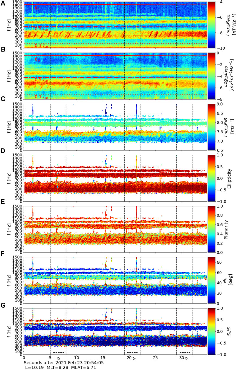
Figure 1. Multiband whistler mode wave event detected by MMS1 on 23 February 2021. Panels show (A) magnetic power spectral density, (B) electric power spectral density, (C) $E/B$ ratio, (D) ellipticity, (E) planarity, (F) wave normal angle, and (G) direction of wave Poynting flux, respectively. The black vertical dashed lines represent the selected time intervals ($t_1$, $t_2$, and $t_3$) for further analysis.

Figure 2

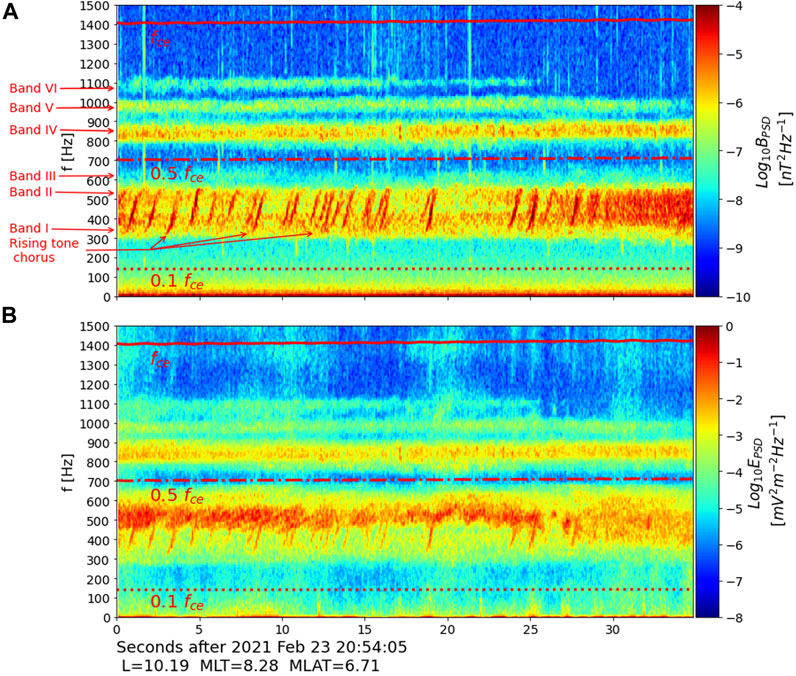
Figure 2. A zoomed-in view of Figure 1A,B displaying the magnetic and electric power spectral densities, respectively. The figure highlights distinct frequency bands and the rising tone chorus of the observed multiband whistler mode wave event.

3 Magnetic amplitude correlation

We discuss here the possible correlation among three bands to investigate the nonlinear coupling between two lower band whistler waves producing an upper band whistler mode wave. In our analysis of the MMS whistler mode wave event, we presented a spectrogram (see Figure 2) that displays three distinct bands: band I, band II, and band IV. For this amplitude correlation analysis, we focus on narrow frequency ranges within these bands with 300 Hz $\le f_1\le$ 350 Hz, 500 Hz $\le f_2\le$ 550 Hz, and 800 Hz $\le f_3\le$ 850 Hz. For identifying possible amplitude correlations, we calculated the magnetic amplitude for each band by integrating magnetic power from $f_{\mathit{peak}}$ −20 Hz to $f_{\mathit{peak}}$ +20 Hz at each time, where $f_{\mathit{peak}}$ is the frequency with the highest power within each band. For most of the observed events, we cannot see any obvious amplitude correlation probably because of rising tone features. However, during the time interval from 23-02-2021/20:54:24.30 to 20:54:29.25, we observed weak evidence of amplitude correlation between the bands, as illustrated in Figure 3. For the first 1.5 s, the magnetic amplitude of $f_3$ shows partial correlation with the effective amplitude, calculated as $\sqrt{\delta B_{f1}\delta B_{f2}}$. From 1.5 to 2.7 s, the correlation becomes relatively stronger, with the amplitude of $f_3$ well aligned with the effective amplitude. Up to 2.7 s, there is a slight shift in the amplitude of $f_3$ band compared to the effective amplitude. After that, the amplitude of this band clearly shifts in time. This amplitude correlation, though not completely clear, apparently shifts in time, indicating that three-wave coupling is possibly happening in a region away from the spacecraft, so that time shift is likely due to different propagation speeds (i.e., group speed).

Figure 3

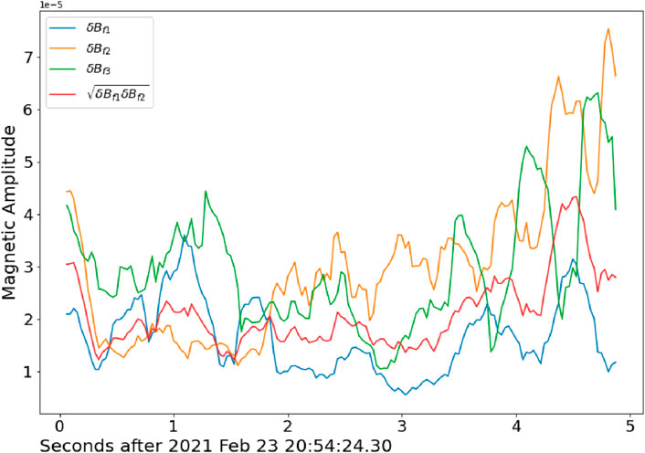
Figure 3. Magnetic amplitude correlation among three bands (band I, band II and band IV). Magnetic amplitude of $f_1$, $f_2$ and $f_3$ are represented by blue, orange and green lines, respectively. The red line denotes the effective magnetic amplitude, $\sqrt{\delta B_{f1}\delta B_{f2}}$.

4 Wavelet bispectrum

We consider two signals $x(t)$ and $y(t)$ to define wavelet bispectrum and as per Milligen et al. (1995a), the bispectrum can be expressed as

$B_{\mathit{xxy}}\left(a_1,a_2\right)=\int W_x\left(a_1,t\right)W_x\left(a_2,t\right)\overline{W_y\left({\left(a_1^{-1}+a_2^{-1}\right)}^{-1},t\right)}dt,(2)$

where the integral is taken over a finite time interval, $I=(T,T+\delta T)$, $a_1$ and $a_2$ are input timescales and $W_x(a_1,t)$ and $W_y(a_2,t)$, are the continuous wavelet transforms of the signals $x(t)$, and $y(t)$, respectively. The basic idea of wavelet transform is to decompose a signal into a set of basis functions named wavelets to extract simultaneous local spectral and temporal information. Note that wavelets are small oscillatory functions with localized features that can be flexibly shifted and scaled to match various characteristics in the signal at different times or scales. Unlike sines or cosines, which have nonzero behaviour over infinite time, wavelets decay rapidly with time.

Milligen et al. (1995a) further defined wavelet bicoherence by normalizing the wavelet bispectrum. The normalized squared bispectrum is the squared wavelet bicoherence (Milligen et al., 1995a) and can be given by,

$b_{\mathit{xxy}}\left(a_1,a_2\right)=\frac{|B_{\mathit{xxy}}\left(a_1,a_2\right){|}^2}{\int |W_x\left(a_1,t\right)W_x\left(a_2,t\right){|}^{2}dt\int |W_y\left({\left(a_1^{-1}+a_2^{-1}\right)}^{-1},t\right){|}^{2}dt}.(3)$

Wavelet bicoherence provides values between 0 and 1 and one can measure coupling between two frequencies satisfying resonance conditions for three-wave interactions when the wavelet bicoherence is close to 1. However, Newman et al. (2021) highlighted the difficulty of describing nonlinear interactions based solely on wavelet bicoherence values. This difficulty arises because estimating wavelet bicoherence using Equation 3 does not clarify whether high bicoherence values represent true interactions between oscillatory influences or simply the absence of oscillatory components and related harmonics. Additionally, while wavelet bicoherence provides information about the bispectral content in scale-scale space, it complicates the interpretation of how this spectral content is distributed across different regions in that space. Seeking a solution to this issue, they introduced the wavelet bispectral density (WBD) by suitable normalization of Equation 2, where the integration of spectral densities is performed over a region of time-frequency-frequency space (or time-scale-scale space) to provide bispectral content of that region.

Newman et al. (2021) assumed an inverse relationship between frequency and scale, $f=\frac{\kappa }{a}$, where $\kappa$ is a constant of proportion. They considered the frequency variable, $f$, as the first argument in the wavelet transform instead of the scale, $a$, which is then used in the definition of WBD. Considering a mother wavelet function $\psi$, we can express the wavelet transform of any $x$ by

$W_{\psi ,k,x}\left(f,t\right)=\frac{f}{\kappa }\underset{\mathbb{R}}{\int }x\left(\tau \right)\overline{\psi \left(\frac{\left(\tau -t\right)f}{\kappa }\right)}d\tau (4)$

for $\kappa >0$, $f>0$ and $t\in \mathbb{R}$. The modulus of $W_{\psi ,k,x}(f,t)$ denotes the wavelet amplitude and the arguments of $W_{\psi ,k,x}(f,t)$ express the wavelet phase related to the frequency, $f$, at time, $t$.

For defining the wavelet bispectrum, a valid candidate can be represented through the integration of a formula for wavelet bispectral density, whose value at $(f_1,f_2,t)$ depends solely on the input signals’ wavelet transforms at time $t$. This suggests that the wavelet bispectrum can act as a time-localized measure of the bispectral content in signals with time-varying oscillatory characteristics. Now, using Equation 4 the wavelet bispectral density (Newman et al., 2021) can be expressed as

$b_{\psi ,k,xxy}\left(f_1,f_2,t\right)=D_{\psi }{\left(f_1,f_2\right)}^{-1}{W}_{\psi ,k,x}\left(f_1,t\right)\times W_{\psi ,k,x}\left(f_2,t\right)\overline{W_{\psi ,k,y}\left(f_1+f_2,t\right)}.(5)$

The normalization factor, $D_{\psi }$, is given by

$D_{\psi }\left(f_1,f_2\right)=\underset{0}{\overset{\infty }{\int }}\underset{0}{\overset{\infty }{\int }}\frac{\widehat{\psi }\left(\frac{f_1}{{\xi }_1}\right)\widehat{\psi }\left(\frac{f_2}{{\xi }_2}\right)\widehat{\psi }\left(\frac{f_1+f_2}{{\xi }_1+{\xi }_2}\right)}{{\xi }_1{\xi }_2}d{\xi }_{1}d{\xi }_2.(6)$

Detailed information about the interpretation of the definition of WBD can be found in Newman et al. (2021).

Note that we are following the methodology and formulae from Newman et al. (2021), so that we are working with a suitably normalized form of the bispectral density. The notation for Equation 6 is slightly different from Equation (46) of Newman et al. (2021) to clarify that it is symmetric under the interchange of $f_1$ and $f_2$. The advantage of this normalization is that the WBD (i.e., implicitly the strength of nonlinear coupling) can be compared across frequency-frequency space and the time variation can be studied consistently. Also, the normalization means that peaks in the WBD are not shifted in frequency-frequency space depending on the relative power of the signals.

5 Applying wavelet bispectrum to real data

We use the Matlab code for the wavelet bispectral analysis methods developed by Newman et al. (2021), Rowland Adams et al. (2021) to study the time evolution of bispectrum using real data. We first test this code by taking data for published events. Gao et al. (2017) studied nonlinear wave-wave coupling between whistler mode waves by considering a THEMIS D event observed on 04 February 2010 at about L-shell 8. They applied the wavelet bicoherence analysis method as described in Milligen et al. (1995a), Milligen et al. (1995b) to estimate nonlinear interaction phenomena for the considered event. Considering similar data, we apply Newman et al. (2021)’s approach to investigate the WBD. Note that we choose combinations of electric field $E_y$ and $E_z$ components for this analysis similar to Gao et al. (2017). Figures 4A, B show results after wavelet transform of $E_y$ and $E_z$ components exhibiting the presence of three bands within the time interval 04-02-2010/03:34:38 - 43.5 s. Figure 4C displays WBD using the idea of Equations 5, 6 for the subinterval (04-02-2010/03:34:40.50 - 40.56 s). Note that the subinterval used here is different from their work where three bands are mostly correlated as can be seen in Figures 4A, B. We can see the presence of high WBD at about $f_1$ = 210 Hz and $f_2$ = 370 Hz indicating the wave-wave coupling process. A large value of WBD is also observed at the diagonal of the frequency-frequency space ($f_1$ = 200 Hz and $f_2$ = 200 Hz), indicating individual nonlinear oscillations of two lower band whistler mode waves. It is noteworthy that the WBD method (Newman et al., 2021) may show different results compared to the bicoherence method (Milligen et al., 1995a) due to the different normalizations of the wavelet bispectrum used in these two methods. Additionally, we refer to Section 3 of Newman et al. (2021), which discusses wavelet bispectra and explains how the normalization of the wavelet bispectrum is used to define WBD. They also describe bicoherence in relation to wavelet bispectral analysis (see their Appendix B). We also observe the variation of WBD at other short subintervals (not shown here) indicating some variabilities in the coupling process. Therefore, the wavelet bispectrum analysis confirms the findings of Gao et al. (2017), and provides further information regarding variability.

Figure 4

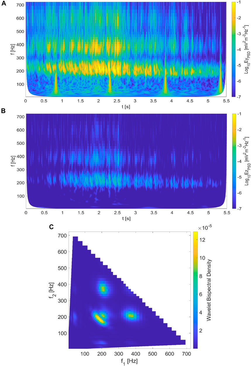
Figure 4. Wavelet analysis of THEMIS D event reported in Gao et al. (2017). Panels (A, B) the $E_y$ and $E_z$ wavelet power spectra for a 5.5 s event and (C) wavelet bispectral density for a short time interval in frequency-frequency space indicating nonlinear coupling phenomena between two whistler mode waves.

Now, we apply Newman et al. (2021)’s approach to examine the MMS multiband whistler mode wave event observed on 23 February 2021. First, we consider three different time intervals ($t_1$, $t_2$, and $t_3$) each of which considered 3 s data for this analysis as shown in Figure 1. For the first interval ($t_1$ = 23-02-2021/20:54:10–13 s), we found the presence of multiband along with rising tone features. Now, we employ wavelet bispectral analysis for this 3 s time interval. We present WBD results considering entire 3 s data (see Figure 5A) and for different short-time subintervals 23-02-2021/20:54:10.5–10.6 s, 10.9–11.0 s, 11.85–11.95 s, 12.38–12.48 s as shown in Figures 5B–E, respectively. We observe several significant peaks in these figures. We are particularly interested in the peak occurring around $f_1$ = 304 Hz and $f_2$ = 528 Hz which is just the mirror point of $f_1$ = 528 Hz and $f_2$ = 304 Hz (see Figure 5A). We can speculate that this peak indicates a nonlinear wave-wave coupling process. We also see a peak on the diagonal of frequency-frequency space which is due to individual nonlinear oscillations rather than nonlinear interactions of oscillations (see Figure 5A). Further, we investigate how the value of the bispectral densities varies at different points in time. Figures 5C, D show the presence of a strong signal while Figures 5B, E exhibit the appearance of a weak signal at the similar location for the considered peak. For the second interval ($t_2$ = 23-02-2021/20:54:24–27 s), we found the presence of multiband whistler without rising tone characteristics. Figure 6 shows wavelet bispectral results for this 3 s data and for four short time subintervals (23-02-2021/20:54:24.2–24.3 s, 25.25–25.35 s, 25.5–25.6 s, 26.1–26.2 s). In this case, we also observe a peak approximately around $f_1$ = 304 Hz and $f_2$ = 528 (see Figure 6A). Further, the value of the bispectral densities varies for this peak when we investigate time-evolving behaviour from WBD results for short time subintervals (see Figures 6B–E). For a particular subinterval, the considered peak becomes weak and overlaps with other peaks as can be seen in Figure 6E. We identified three significant peaks in Figure 6A, including one peak ($f_1$ = 304 Hz and $f_2$ = 528 Hz and their mirror peak) that signifies nonlinear interactions between band I and band II. Another peak along the diagonal of the frequency-frequency space suggests the potential influence of individual nonlinear oscillations of these bands. Additionally, to explore how these results are physically meaningful, we investigate the time-varying feature of bispectral content (see Figures 6B–E), which indicates how the nature of interactions between these bands varies in short time intervals (i.e., 100 ms) within the whole time interval (i.e., 3 s). We can observe that the nonlinear coupling peaks are present in all of the subintervals, although with varying strength, which indicates that they are statistically significant. Notably, we selected combinations of the electric field components $E_x$ and $E_z$ for this analysis. Figure 6A shows the time-averaged bispectral density (units of ${mV}^3$ $m^{-3}$), while other panels show the time-evolving bispectral density (units of ${mV}^3{m}^{-3}$ s). Consequently, we observe variations in WBD across the identified peaks, either indicating coupling phenomena or individual nonlinear oscillations when comparing Figure 6A with Figure 6B–E. In order to further understand the results shown in Figure 6, we refer to Section 6 (particularly Figures 16 and 17) of Newman et al. (2021), which discusses the wavelet bispectrum of experimental time series data.

Figure 5

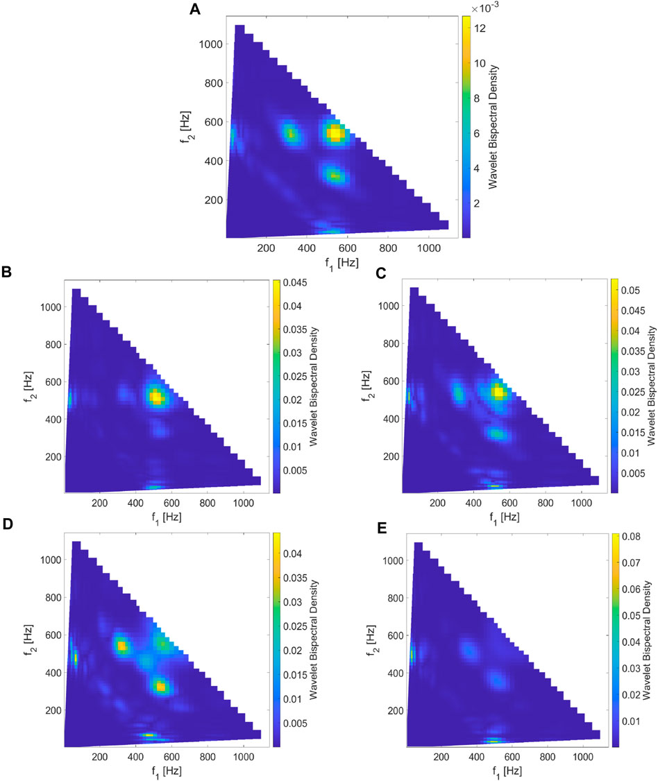
Figure 5. Wavelet bispectral density evaluated in two scenarios: (A) time-averaged bispectral density (units of ${mV}^3$ $m^{-3}$) over the entire 3 s period (time interval, $t_1$), and (B–E) time-evolving bispectral density (units of ${mV}^3$ $m^{-3}$ s) across distinct time subintervals, each spanning 100 ms, within this 3 s period.

Figure 6

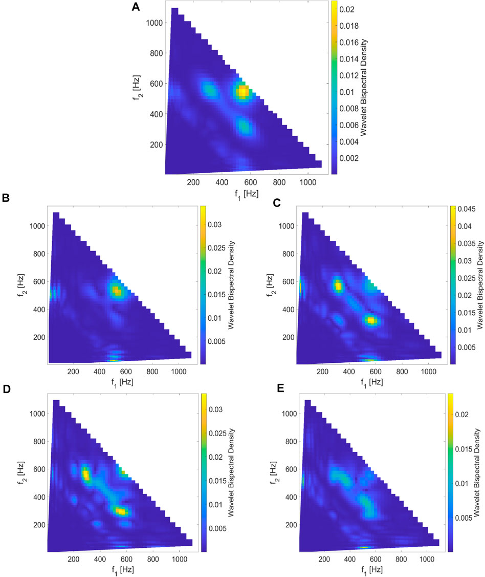
Figure 6. Wavelet bispectral density estimated for another 3 s data (time interval, $t_2$): (A) time-averaged bispectral density (units of ${mV}^3$ $m^{-3}$) over the entire 3 s data, and (B–E) time-evolving bispectral density (units of ${mV}^3$ $m^{-3}$ s) across different time subintervals, each spanning 100 ms, within this 3 s data.

Finally, we examine the time interval ($t_3$ = 23-02-2021/20:54:34 - 37 s) for the WBD analysis. In the initial second, both band I and band II are still observable. However, over time, these bands seem to be overlapped by other emissions. Now, we present results for this whole time interval (see Figure 7A) and for short time subintervals (23-02-2021/20:54:34.3–34.4 s, 35.15–35.25 s, 36.18–36.28 s, 36.65–36.75 s) (see Figures 7B–E). The peak considered in the previous two time intervals ($t_1$ and $t_2$) has either disappeared or shifted, as depicted in Figure 7A. Due to the presence of distinct bands at the beginning of this time interval, we can still observe the considered peak depicted in Figure 7B from WBD analysis. However, in other subintervals, we cannot find any signature of coupling in bispectral densities. Until the start of time interval, $t_3$, band I and band II are well separated by a power gap. However, during $t_3$, the power gap seems to gradually reduce, and both bands appear to overlap by dense intermittent rising tone structures. This is probably why we cannot see clear evidence of coupling from bispectral densities in all subintervals within $t_3$ except one case, as shown in Figure 7B.

Figure 7

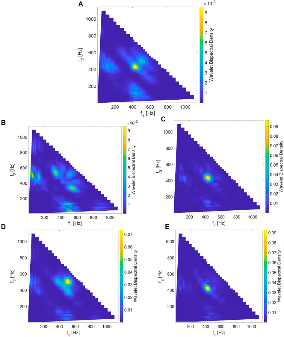
Figure 7. Similar plots to Figure 5, 6, except for the wavelet bispectral density evaluated for the time interval, $t_3$. Plots show results for (A) the whole 3 s data and (B–E) four different 100 ms time subintervals within this 3 s data.

6 Discussion

In this paper, we report the presence of a complex multiband whistler mode wave event in the dayside outer magnetosphere using MMS waveform data. This multiband whistler event comprises distinct bands, each of which exhibits distinguishable characteristics. These characteristics have been identified in terms of magnetic power spectral density, electric power spectral density, $E/B$ ratio, ellipticity, planarity, wave normal angle, and the sign of the Poynting flux parallel to the background magnetic field, respectively. In this event, the lower band and upper band whistler mode waves are found to be either quasi-parallel or oblique with respect to the background magnetic field. Moreover, the waves are observed to propagate in either direction (i.e., northward or southward) after being generated close to the magnetic equator.

The generation mechanism of observed multiband emissions cannot be easily explained with a linear or quasi-linear approach. The intricate characteristics of the wave generation imply that a nonlinear wave interaction mechanism may be more relevant for comprehending such phenomena. To investigate the nonlinear three-wave interaction in the observed multiband whistler event, we employ bispectral analysis on MMS burst mode data for this event. To achieve this, we utilize the wavelet bispectrum analysis method developed by Newman et al. (2021), where they introduced a suitable normalization for the wavelet bispectrum to define the WBD. Note that WBD provides a detailed view of the bispectrum, allowing us to interpret possible nonlinear three-wave interactions that may not be clearly explainable in terms of Fourier bicoherence. WBD also overcomes the limitations of wavelet bicoherence by normalizing the bispectrum in a more efficient manner. The analysis of wavelet bispectral densities in the data for the observed event exhibit several significant peaks in the frequency-frequency space. We identify a peak with a high bispectral density that occurs at a location where the resonance condition for three waves (i.e., $f_3$ = $f_1$ + $f_2$) is satisfied. From this, we can conclude that a wave-wave coupling phenomenon is taking place between two whistler mode lower band waves, giving rise to a whistler mode upper band wave. Further, the observed whistler event contains multiple bands and shows rising tone features. In this study, we investigated three-wave coupling phenomena by considering only the multiband nature of whistler mode waves. In our analysis, we did not find any identifiable bispectrum signature linked to rising tones. The point is that rising tones are not formed by three-wave interaction, so we should not expect to see a bispectrum signature. Also, the short-lived rising tones would be difficult to analyze in terms of WBD. However, additional work might be possible to investigate the broader links between rising tone emission and multiple band events.

The propagation direction of the whistler mode waves is particularly important for the occurrence of the nonlinear coupling process, in order to assess the matching conditions necessary for a three-wave interaction. Teng et al. (2018) reported a lower band chorus wave generated by a nonlinear three-wave interaction, where two parent whistler waves and the produced daughter whistler wave propagate in the same direction. Furthermore, Gao et al. (2017) addressed that nonlinear coupling between two oppositely propagating whistler mode lower band waves can produce an upper band whistler wave, which propagates in the same direction as the relatively higher-frequency lower band wave. However, our present study shows that two lower band whistler mode waves (band I and band II) propagating in the same direction can interact nonlinearly and produce an upper band whistler mode wave (band IV), which propagates in the same direction as both of lower band whistler mode waves.

For the observed multiband event, one can think of generating a lower band whistler wave (band I) by nonlinear coupling between two upper band whistler waves (band VI and band IV). Teng et al. (2018) showed that a lower band chorus wave can be generated by two copropagating whistler mode waves by satisfying the matching condition ${\omega }_3={\omega }_1-{\omega }_2$ necessary for a nonlinear three-wave interaction. In the case of our event, the reason for not producing such a lower band whistler wave might be related to the propagation direction and the strength of the upper band whistler mode waves. From the wave characteristics discussed in Section 2, it is found that band VI and band IV are counter-propagating, unlike the observation by Teng et al. (2018). In addition, band VI is very weak (roughly 100 times weaker than band IV in terms of E-PSD) and not continuous throughout the observation period of the event in comparison to band IV. Therefore, although the frequency difference between band VI and band IV closely matches the frequency of band I, nonlinear three-wave interaction does not occur between band VI and band IV to produce a daughter wave such as band I.

Our study focuses on the wave-wave coupling phenomena in multiband whistler mode waves. Specifically, we investigate how two lower band whistler mode waves interact to produce an upper band whistler mode wave. To validate this wave-wave coupling mechanism, we also performed a wave vector analysis to determine whether the resonance condition ($k_3$ = $k_1$ + $k_2$ in Equation 1) among the wave vectors of three bands (band I, band II, and band IV, or band I, band III, and band IV) is satisfied. Gao et al. (2017) used the cold plasma linear dispersion relation between frequency and wave vector to test the wave vector resonance condition by using observed propagation properties of $k_1$ and $k_2$ to predict the wave propagation angle for $k_3$. We have used the same method, and for the interaction between band I and band II to form band IV, the predicted propagation angle of $k_3$ is in the approximate range of [5, 20] degrees, whereas the observed angle is approximately 40°, with variability in the range of [30, 50] degrees. This is for the case which matches the observations with $k_1$ and $k_2$ co-propagating (i.e., in the same sense of parallel propagation). If, hypothetically, we assume they are counter-propagating, there is better agreement with the predicted propagation angle of $k_3$, which is in the range of [30, 60] degrees. We have also examined the interaction between band I and band III to form band IV, which has a fairly close frequency match and found that the predicted propagation angle of $k_3$ is in the approximate range of [70, 75] degrees. Thus, we find that the wave vector resonance condition is not perfectly satisfied, but rather is close to being satisfied, with a discrepancy in the propagation angle of 10–20° at best. A closer match is possible if, hypothetically, some component of band I is actually counter-propagating to band II. This might be possible given that the methods for the wave propagation assume a single propagation angle at a given frequency. An alternative explanation is that the resonance condition is perhaps satisfied non-locally, and the observed waves propagate to the observation point but still retain the signature of nonlinear coupling in the bispectrum.

In summary, three-wave coupling can explain some of the observed bands, but other processes are required for a full explanation, such as the generation of pump waves (probably by linear instability), the generation of rising tones (through nonlinear resonance processes), and propagation effects. Note that amplitude correlation discussed in Section 3 does not strictly indicate the region where three-wave coupling is operating, so there is a possibility that the bispectrum signature is the result of a three-wave coupling process happening remote to the observation point. This could also explain the variability seen in the three-wave WBD signature. Finally, the observed multiband event will probably require a complex combination of processes to be fully explained.

Data availability statement

Publicly available datasets were analyzed in this study. This data can be found here: https://lasp.colorado.edu/mms/sdc/public/about/.

Author contributions

MS: Conceptualization, Formal Analysis, Investigation, Methodology, Software, Validation, Visualization, Writing–original draft, Writing–review and editing. DB: Project administration, Supervision, Writing–review and editing.

Funding

The authors declare that financial support was received for the research, authorship, and/or publication of this article. This work was funded by the Commonwealth Scholarship Commission in the UK through a Commonwealth PhD Scholarship. This work also received support from UK STFC grant ST/X000974/1.

Acknowledgments

MS acknowledges funding from the Commonwealth Scholarship Commission in the UK and DB acknowledges funding from UK STFC grant ST/X000974/1. This work used MATLAB code which is available at https://doi.org/10.5281/zenodo.5519692. The MMS data used in this study is available at the MMS Science Data Center https://lasp.colorado.edu/mms/sdc/public/about/.

Conflict of interest

The authors declare that the research was conducted in the absence of any commercial or financial relationships that could be construed as a potential conflict of interest.

Publisher’s note

All claims expressed in this article are solely those of the authors and do not necessarily represent those of their affiliated organizations, or those of the publisher, the editors and the reviewers. Any product that may be evaluated in this article, or claim that may be made by its manufacturer, is not guaranteed or endorsed by the publisher.

References

Bale, S. D., Burgess, D., Kellogg, P. J., Goetz, K., Howard, R. L., and Monson, S. J. (1996). Phase coupling in Langmuir wave packets: possible evidence of three-wave interactions in the upstream solar wind. Geophys. Res. Lett. 23, 109–112. doi:10.1029/95GL03595

CrossRef Full Text | Google Scholar

Bortnik, J., Inan, U. S., and Bell, T. F. (2006). Landau damping and resultant unidirectional propagation of chorus waves. Geophys. Res. Lett. 33, L03102. doi:10.1029/2005GL024553

CrossRef Full Text | Google Scholar

Bortnik, J., Thorne, R. M., and Meredith, N. P. (2008). The unexpected origin of plasmaspheric hiss from discrete chorus emissions. Nature 452, 62–66. doi:10.1038/nature06741

PubMed Abstract | CrossRef Full Text | Google Scholar

Burtis, W. J., and Helliwell, R. A. (1969). Banded chorus–A new type of VLF radiation observed in the magnetosphere by OGO 1 and OGO 3. J. Geophys. Res. 74, 3002–3010. doi:10.1029/JA074i011p03002

CrossRef Full Text | Google Scholar

Burton, R. K., and Holzer, R. E. (1974). The origin and propagation of chorus in the outer magnetosphere. J. Geophys. Res. 79, 1014–1023. doi:10.1029/JA079i007p01014

CrossRef Full Text | Google Scholar

Chen, R., Gao, X., Chen, H., and Wang, S. (2020). A new generation mechanism of three-band chorus waves in the Earth’s magnetosphere. J. Univ. Sci. Technol. China 50, 1249–1257. doi:10.3969/j.issn.0253-2778.2020.09.004

CrossRef Full Text | Google Scholar

Contel, O. L., Leroy, P., Roux, A., Coillot, C., Alison, D., Bouabdellah, A., et al. (2016). The search-coil magnetometer for MMS. Space Sci. Rev. 199, 257–282. doi:10.1007/s11214-014-0096-9

CrossRef Full Text | Google Scholar

Dudok de Wit, T., and Krasnosel’skikh, V. V. (1995). Wavelet bicoherence analysis of strong plasma turbulence at the Earth’s quasiparallel bow shock. Phys. Plasmas 2, 4307–4311. doi:10.1063/1.870985

CrossRef Full Text | Google Scholar

Ergun, R. E., Tucker, S., Westfall, J., Goodrich, K. A., Malaspina, D. M., Summers, D., et al. (2016). The axial double probe and fields signal processing for the MMS mission. Space Sci. Rev. 199, 167–188. doi:10.1007/s11214-014-0115-x

CrossRef Full Text | Google Scholar

Fu, X., Gary, S. P., Reeves, G. D., Winske, D., and Woodroffe, J. R. (2017). Generation of highly oblique lower band chorus via nonlinear three-wave resonance. Geophys. Res. Lett. 44, 9532–9538. doi:10.1002/2017GL074411

CrossRef Full Text | Google Scholar

Fu, X., Guo, Z., Dong, C., and Gary, S. P. (2015). Nonlinear subcyclotron resonance as a formation mechanism for gaps in banded chorus. Geophys. Res. Lett. 42, 3150–3159. doi:10.1002/2015GL064182

CrossRef Full Text | Google Scholar

Gao, X., Li, W., Thorne, R. M., Bortnik, J., Angelopoulos, V., Lu, Q., et al. (2014). New evidence for generation mechanisms of discrete and hiss-like whistler mode waves. Geophys. Res. Lett. 41, 4805–4811. doi:10.1002/2014GL060707

CrossRef Full Text | Google Scholar

Gao, X., Lu, Q., Bortnik, J., Li, W., Chen, L., and Wang, S. (2016). Generation of multiband chorus by lower band cascade in the Earth’s magnetosphere. Geophys. Res. Lett. 43, 2343–2350. doi:10.1002/2016GL068313

CrossRef Full Text | Google Scholar

Gao, X., Lu, Q., and Wang, S. (2017). First report of resonant interactions between whistler mode waves in the Earth’s magnetosphere. Geophys. Res. Lett. 44, 5269–5275. doi:10.1002/2017GL073829

CrossRef Full Text | Google Scholar

Gao, Z., Zou, Z., Zuo, P., Wang, Y., He, Z., and Wei, F. (2019). Low-frequency hiss-like whistler-mode waves generated by nonlinear three-wave interactions outside the plasmasphere. Phys. Plasmas 26, 122901. doi:10.1063/1.5115542

CrossRef Full Text | Google Scholar

Hagihira, S., Takashina, M., Mori, T., Mashimo, T., and Yoshiya, T. (2021). Practical issues in bispectral analysis of electroencephalographic signals. Anesth. Analg. 93, 966–970. doi:10.1097/00000539-200110000-00032

PubMed Abstract | CrossRef Full Text | Google Scholar

Helliwell, R. A. (1969). Low-frequency waves in the magnetosphere. Rev. Geophys. 7, 281–303. doi:10.1029/RG007i001p00281

CrossRef Full Text | Google Scholar

Kennel, C. F., and Petschek, H. E. (1966). Limit on stably trapped particle fluxes. J. Geophys. Res. 71, 1–28. doi:10.1029/JZ071i001p00001

CrossRef Full Text | Google Scholar

Kim, Y. C., and Powers, E. J. (1979). Digital bispectral analysis and its applications to nonlinear wave interactions. IEEE Trans. Plasma Sci. 7, 120–131. doi:10.1109/TPS.1979.4317207

CrossRef Full Text | Google Scholar

Li, W., Thorne, R. M., Bortnik, J., Tao, X., and Angelopoulos, V. (2012). Characteristics of hiss-like and discrete whistler-mode emissions. Geophys. Res. Lett. 39, L18106. doi:10.1029/2012GL053206

CrossRef Full Text | Google Scholar

Lindqvist, P.-A., Olsson, G., Torbert, R. B., King, B., Granoff, M., Rau, D., et al. (2016). The Spin-Plane Double Probe electric field instrument for MMS. Space Sci. Rev. 199, 137–165. doi:10.1007/s11214-014-0116-9

CrossRef Full Text | Google Scholar

Macúšová, E., Santolík, O., Cornilleau-Wehrlin, N., Pickett, J. S., and Gurnett, D. A. (2014). Multi-banded structure of chorus-like emission, in 2014 XXXIth URSI general assembly and scientific symposium (URSI GASS). Beijing, China, August 16–23, 2014 (IEEE), 1–4.

Google Scholar

Milligen, B. P. V., Hidalgo, C., and Sã¡nchez, E. (1995a). Nonlinear phenomena and intermittency in plasma turbulence. Phys. Rev. Lett. 74, 395–398. doi:10.1103/PhysRevLett.74.395

PubMed Abstract | CrossRef Full Text | Google Scholar

Milligen, B. P. V., Sánchez, E., Estrada, T., Hidalgo, C., Brañas, B., Carreras, B., et al. (1995b). Wavelet bicoherence: a new turbulence analysis tool. Phys. Plasmas 2, 3017–3032. doi:10.1063/1.871199

CrossRef Full Text | Google Scholar

Newman, J., Pidde, A., and Stefanovska, A. (2021). Defining the wavelet bispectrum. Appl. Comput. Harmon. Analysis 51, 171–224. doi:10.1016/j.acha.2020.10.005

CrossRef Full Text | Google Scholar

Ni, B., Li, W., Thorne, R. M., Bortnik, J., Ma, Q., Chen, L., et al. (2014). Resonant scattering of energetic electrons by unusual low-frequency hiss. Geophys. Res. Lett. 41, 1854–1861. doi:10.1002/2014GL059389

CrossRef Full Text | Google Scholar

Rowland Adams, J., Piddle, A., Newman, J., and Stefanovska, A. (2021). Bispectrum testing. doi:10.5281/zenodo.5519691

CrossRef Full Text | Google Scholar

Russell, C. T., Anderson, B. J., Baumjohann, W., Bromund, K. R., Dearborn, D., Fischer, D., et al. (2016). The magnetospheric Multiscale magnetometers. Space Sci. Rev. 199, 189–256. doi:10.1007/s11214-014-0057-3

CrossRef Full Text | Google Scholar

Santolík, O., Gurnett, D. A., Pickett, J. S., Chum, J., and Cornilleau-Wehrlin, N. (2009). Oblique propagation of whistler mode waves in the chorus source region. J. Geophys. Res. 114, A00F03. doi:10.1029/2009JA014586

CrossRef Full Text | Google Scholar

Santolík, O., Parrot, M., and Lefeuvre, F. (2003). Singular value decomposition methods for wave propagation analysis. Radio Sci. 38, 1010. doi:10.1029/2000RS002523

CrossRef Full Text | Google Scholar

Santolík, O., Pickett, J. S., Gurnett, D. A., Menietti, J. D., Tsurutani, B. T., and Verkhoglyadova, O. (2010). Survey of Poynting flux of whistler mode chorus in the outer zone. J. Geophys. Res. Space Phys. 115, A00F13. doi:10.1029/2009JA014925

CrossRef Full Text | Google Scholar

Schriver, D., Ashour-Abdalla, M., Coroniti, F. V., LeBoeuf, J. N., Decyk, V., Travnicek, P., et al. (2010). Generation of whistler mode emissions in the inner magnetosphere: an event study. J. Geophys. Res. Space Phys. 115, A00F17. doi:10.1029/2009JA014932

CrossRef Full Text | Google Scholar

Summers, D., Omura, Y., Nakamura, S., and Kletzing, C. A. (2014). Fine structure of plasmaspheric hiss. J. Geophys. Res. Space Phys. 119, 9134–9149. doi:10.1002/2014JA020437

CrossRef Full Text | Google Scholar

Taubenschuss, U., Santolík, O., Breuillard, H., Li, W., and Contel, O. L. (2016). Poynting vector and wave vector directions of equatorial chorus. J. Geophys. Res. Space Phys. 121 (11), 11–928. doi:10.1002/2016JA023389

CrossRef Full Text | Google Scholar

Teng, S., Zhao, J., Tao, X., Wang, S., and Reeves, G. D. (2018). Observation of oblique lower band chorus generated by nonlinear three-wave interaction. Geophys. Res. Lett. 45, 6343–6352. doi:10.1029/2018GL078765

CrossRef Full Text | Google Scholar

Tsurutani, B. T., and Smith, E. J. (1974). Postmidnight chorus: a substorm phenomenon. J. Geophys. Res. 79, 118–127. doi:10.1029/JA079i001p00118

CrossRef Full Text | Google Scholar

Tsurutani, B. T., and Smith, E. J. (1977). Two types of magnetospheric elf chorus and their substorm dependences. J. Geophys. Res. 82, 5112–5128. doi:10.1029/JA082i032p05112

CrossRef Full Text | Google Scholar

Vaivads, A., Santolík, O., Stenberg, G., André, M., Owen, C. J., Canu, P., et al. (2007). Source of whistler emissions at the dayside magnetopause. Geophys. Res. Lett. 34, L09106. doi:10.1029/2006GL029195

CrossRef Full Text | Google Scholar