Short-term prediction of horizontal winds in the mesosphere and lower thermosphere over coastal Peru using a hybrid model

The mesosphere and lower thermosphere (MLT) are transitional regions between the lower and upper atmosphere. The MLT dynamics can be investigated using wind measurements conducted with meteor radars. Predicting MLT winds could help forecast ionospheric parameters, which has many implications for global communications and geo-location applications. Several literature sources have developed and compared predictive models for wind speed estimation. However, in recent years, hybrid models have been developed that significantly improve the accuracy of the estimates. These integrate time series decomposition and machine learning techniques to achieve more accurate short-term predictions. This research evaluates a hybrid model that is capable of making a short-term prediction of the horizontal winds between 80 and 95 km altitudes on the coast of Peru at two locations: Lima (12°S, 77°W) and Piura (5°S, 80°W). The model takes a window of 56 data points as input (corresponding to 7 days) and predicts 16 data points as output (corresponding to 2 days). First, the missing data problem was analyzed using the Expectation Maximization algorithm (EM). Then, variational mode decomposition (VMD) separates the components that dominate the winds. Each resulting component is processed separately in a Long short-term memory (LSTM) neural network whose hyperparameters were optimized using the Optuna tool. Then, the final prediction is the sum of the predicted components. The efficiency of the hybrid model is evaluated at different altitudes using the root mean square error (RMSE) and Spearman’s correlation (r). The hybrid model performed better compared to two other models: the persistence model and the dominant harmonics model. The RMSE ranged from 10.79 to 27.04 ${\mathrm{m}\mathrm{s}}^{-1}$, and the correlation ranged from 0.55 to 0.94. In addition, it is observed that the prediction quality decreases as the prediction time increases. The RMSE at the first step reached 6.04 ${\mathrm{m}\mathrm{s}}^{-1}$ with a correlation of 0.99, while at the sixteenth step, the RMSE increased up to 30.84 ${\mathrm{m}\mathrm{s}}^{-1}$ with a correlation of 0.5.

1 Introduction

The mesosphere and lower thermosphere (MLT) is the region of coupling between the lower and upper atmosphere. It is a region of complex chemical processes and dynamics (Liu et al., 2021). Understanding of this region is still in progress and it is of interest in atmospheric science and space traffic management.

The MLT dynamics is characterized by waves of different scales generated by other sources. For instance, on planetary scales, it is characterized by solar tides and planetary waves. The solar tides present periods of subharmonics of solar days and are generated mainly by the solar radiation absorption of tropospheric water vapor and stratospheric ozone (Forbes, 1995). On the other hand, the planetary waves have periods of days, e.g., the quasi-two-day waves with periods of 2 days generated in situ by baroclinic instabilities (McCormack et al., 2014). Moreover, the mesoscale gravity waves have periods of minutes to hours and can be generated by orographic sources and deep convection (Piani et al., 2000).

The MLT dynamics has usually been investigated using global circulation models (e.g., Liu et al., 2018), rockets (e.g., Staszak et al., 2021), satellites (e.g., Gasperini et al., 2023), lidars (e.g., Emmert et al., 2021), and radars (e.g., Chau et al., 2021). On the central and northern coast of Peru, two multi-static meteor radar networks, SIMONe Jicamarca (12°S, 77°W) in Lima and SIMONe Piura (5°S, 80°W) in Piura, allow us to measure winds between 75 and 105 km altitude since 2019 and 2021, respectively (Chau et al., 2021). Recently, diverse investigations have been conducted in the low-latitude Peruvian sector. For example, Suclupe et al. (2023) studied the climatology of large-scale dynamics, and Conte et al. (2024) studied the mesoscale dynamics.

The MLT region at low latitudes is significant for studying the effect of the lower atmospheric forces on the ionosphere (Immel et al., 2006; Vincent, 2015), a region with important implications for global communications and geo-location applications.

From another point of view, Yang et al. (2023) mention that near space (between 20 and 100 km altitude) is frequented by various aerospace vehicles. Like other research, they describe that there are complex dynamic processes, but emphasize that neutral atmospheric wind is a critical atmospheric parameter that influences the design and construction of aerospace vehicles. They argue that accurate wind prediction at these altitudes is essential for aerospace research. Similarly, Dhadly et al. (2023) mention that the upper atmosphere (between 85 and 500 km altitude) has complex dynamics and that the behavior of the climate in this region directly impacts communication and navigation technologies that are important to humanity. They add that, due to our increasing dependence on these space technologies, predicting the dynamics in the upper atmosphere will become increasingly important.

In wind predictive models, several investigations have been carried out mainly at the tropospheric level (e.g., Hussin et al., 2021; Hanifi et al., 2022). These investigations usually use two types of models: statistical and machine learning models. Hussin et al. (2021) mention that there are statistical models such as autoregressive (AR), moving average (MA), autoregressive moving average (ARMA), autoregressive Integrated Moving Average (ARIMA), generalized autoregressive conditional heteroskedasticity (GARCH), and ARIMA-GARCH. However, statistical models require the assumption of constant variance, and the original wind speed data do not meet this assumption. Hanifi et al. (2022) highlight that machine learning models are more appropriate methods for this data and that their success depends on an adequate selection of hyperparameters. They argue that the integrated use of Long Short-Term Memory (LSTM) neural networks and the hyperparameter optimizer Optuna accelerates the optimal choice of hyperparameters and gives more accurate estimates.

Recently, a time series decomposition technique called variational mode decomposition (VMD) has been introduced. This technique is applied before statistical modeling or modeling with machine learning and helps to deal with the problem of high variability. Ali et al. (2018) evaluate the application of this technique with two models for 1-step, 5-step, and 10-step forecasting horizons. In the first method, they use VMD with the ARIMA model. The second method uses VMD with artificial neural networks (ANN). These prediction methods are compared with other hybrid models such as empirical mode decomposition (EMD) with ARIMA, EMD with ANN, ensemble empirical mode decomposition (EEMD) with ARIMA, EEMD with ANN, complete ensemble empirical mode decomposition with Adaptive Noise (CEEMDAN) with ARIMA, and CEEMDAN with ANN. They conclude that the integration of VMD with ARIMA and VMD with ANN significantly outperforms existing hybrid models, for all prediction horizons.

In the prediction of wind speeds in the MLT region, Yang et al. (2023) also propose to use VMD before inputting the data into the prediction model. They used the hybrid VMD- PSO-LSTM model, which can decompose the wind time series for more accurate predictions. To do this, they used the VMD technique, which decomposes the original time series into principal components that dominate the signal. Then, each component is fed into the LSTM neural network, which finds the best hyperparameter values with the help of the particle swarm optimization (PSO) algorithm. This methodology is compared with the seasonal auto-regressive integrated moving average (SARIMA) statistical model and the hybrid models EMD-PSO-LSTM, EEMD-PSO-LSTM, CEEMDAN-PSO-LSTM and VMD-PSO-LSTM. Time horizons of 1 step, 3 steps, and 5 steps are predicted. They conclude that the proposed method has better efficiency and stability in wind speed prediction in all their comparisons.

This research studies the predictability of the mesospheric and lower thermospheric winds. In Peru, this prediction analysis has already been developed by Mauricio et al. (2023), whose model is based on the methodology used by Yang et al. (2023). The techniques used are missing data imputation, time series decomposition, and deep learning. These can identify the main components of the winds and then perform better predictions. Mauricio et al. (2023) modified the methodology of Yang et al. (2023). They added a missing data imputation analysis and used the Optuna hyperparameter optimizer in the modeling because it offers a better way to analyze the model quality.

The present research is a continuation of the work carried out by Mauricio et al. (2023). A new decomposition of the time series and a new hyperparameter search with Optuna have been performed. The main objective is to compare the efficiency of the hybrid model with a model of dominant harmonics based on the MLT climatology over Peru. The intention is to demonstrate that the hybrid model gives more accurate predictions. This will be evaluated with the root mean square error (RMSE) and nonparametric Spearman correlation (r).

2 Materials and methods

2.1 Original data set

The zonal and meridional winds were estimated using the homogeneous method (e.g., Chau et al., 2021) recorded by SIMONe (Spread-spectrum Interferometric Multistatic meteor radar Observing Network) radars in Lima (12°S, 77°W) and Piura (5°S, 80°W). These systems have a horizontal coverage of approximately 400 km in diameter (Chau et al., 2021). The horizontal winds have a resolution of 1-h, and 2-km and were estimated every 30-min and 1-km (sampling) at heights of 80.5 km, 85.5 km, 90.5 km, and 95.5 km.

The available data for the Lima and Piura stations is described on Table 1. The period is different because the stations started operating in different years. The data sets are divided into two parts. The first part is used for model development, covering the training, validation and testing stages. In the case of Lima, the period runs from September 2020 to November 2021. In the case of Piura, the period runs from October 2021 to December 2022. In both cases, those periods were chosen since they have the same amount of records so that the modeling would be similar, although they differ on the amount of missing data (Figure 1).

Table 1

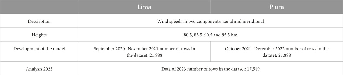
Table 1. Original data set.

Figure 1

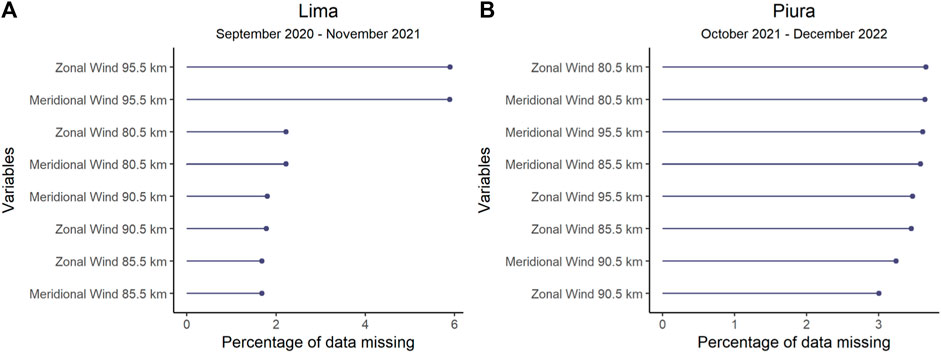
Figure 1. Missing data at the model development stage. (A) shows the percentage of missing data in Lima. (B) shows the percentage of missing data in Piura.

In the second part, the performance of the proposed model is evaluated in both stations using data from the year 2023. In this section, the number of records and the period coincide, but they differ on the amount of missing data (Figure 2).

Figure 2

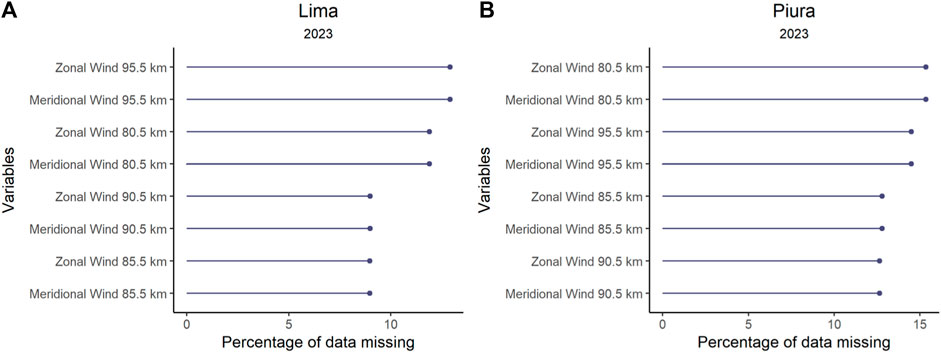
Figure 2. Missing data in the year 2023. (A) presents the percentage of missing data in Lima. (B) shows the percentage of missing data in Piura.

2.2 Missing data imputation

Missing data imputation was performed using the Expectation–maximization (EM) algorithm, which applies to data following a Gaussian distribution. This algorithm is used to estimate the parameters of a probability distribution from incomplete data by iteratively maximizing the likelihood of the available data. In the context of multivariate Gaussian data, the probability distribution can be characterized by the vector of means and the variance-covariance matrix (Schneider, 2001).

The EM algorithm has two stages: the E-step, which assumes the population mean and variance are known, and the M-step, which uses these values to estimate the population mean and covariance matrix. This iteration process continues until the parameter estimates of interest no longer change significantly. Maximum likelihood methods for incomplete multivariate data, particularly in the case of normally distributed data, focus on estimating the observed data parameters, such as the vector of means and the variance-covariance matrix. If the data follow a multivariate normal distribution, one can apply known properties to estimate those unknown parameters (Pigott, 2001).

The imputation analysis consisted of two parts. First, the imputation procedure described by Mauricio et al. (2023) was replicated. Additionally, the descriptive statistical indicators were presented to comprehend the process better. The second part involved exclusively imputing data from the year 2023, because these were obtained at a later point in time. Figure 2 shows the percentages of missing data for the year 2023, for the Lima and Piura stations. The absence of data was mainly due to two reasons. First, during the first months of the year, the equipment was affected by the presence of heavy rains in the region, caused by cyclone Yaku and the El Niño Costero phenomenon. Secondly, during the year, there were some radar hardware failures. These unexpected situations forced the radars to be inoperative at certain intervals.

In case of high percentages of missing data, the time series is partitioned in such a way as to omit the time intervals with accumulated absences. The maximum percentage limit allowed in each subseries is 6%, which is an approximate value of that detected in the article of Mauricio et al. (2023). Then, for each subseries, the percentage is reanalyzed. If the percentage is less than 6%, we proceed with the estimation of the missing data. Otherwise, the time subseries are further separated until their percentages are lower than 6%.

2.3 Data preprocessing

Once the missing data are imputed, they are averaged every 3 h. Data not belonging to the year 2023 are divided chronologically into train (70%), validation (10%) and test (20%). Training and validation data are used for the building and optimization of the model, while the test data is used specifically for the metric evaluation. The intention is that the test data is not involved in the modeling and optimization, to avoid overfitting (Mauricio et al., 2023). Finally, each data block is normalized based on the training data, before moving on to the time series decomposition stage.

2.4 Time serie decomposition

Variational mode decomposition (VMD) is a method used in signal processing. This method was proposed in 2014 to overcome the limitations of techniques such as wavelet analysis and Empirical Mode Decomposition (EMD). The VMD technique decomposes a sequence, such as wind time series, into multiple sub-sequences known as intrinsic modal function (IMF) components. The importance of VMD is its ability to optimally adapt the center frequency and bandwidth of each IMF according to the signal characteristics, which makes it effective in dealing with non-smoothness in data series, such as wind speed data (Yang et al., 2023). The VMD algorithm has as input a signal or time series $\mathrm{x}\left(\mathrm{t}\right)$, which is decomposed into subseries called modes or harmonic signals ${\mathrm{u}}_{\mathrm{k}}\left(\mathrm{t}\right)$, where k is the number of total modes.

$\mathbf{x}\left(\mathbf{t}\right)={\displaystyle \sum _{\mathbf{k}=\mathbf{1}}^{\mathbf{K}}}{\mathbf{u}}_{\mathbf{k}}\left(\mathbf{t}\right)$

${\mathbf{u}}_{\mathbf{k}}={\mathbf{A}}_{\mathbf{k}}\left(\mathbf{t}\right)\mathbf{cos}\left({\mathbf{\varphi }}_{\mathbf{k}}\left(\mathbf{t}\right)\right)$

Each mode has an instantaneous amplitude ${\mathrm{A}}_{\mathrm{k}}\left(\mathrm{t}\right)$, an instantaneous phase ${\mathrm{\varphi }}_{\mathrm{k}}\left(\mathrm{t}\right)$, a limited spectral bandwidth $\mathrm{B}\left({\mathrm{u}}_{\mathrm{k}}\left(\mathrm{t}\right)\right)$ and an instantaneous center frequency ${\mathrm{\omega }}_{\mathrm{k}}$ (Ali, Khan, and Rehman, 2018), where it is assumed that each mode varies slower than the phase and is non-negative (Gan et al., 2021). The complete mathematical process that follows this decomposition and bandwidth estimation can be found in the article of Dragomiretskiy and Zosso (2014).

The VMD algorithm package in Python was obtained from the code developed by Carvalho et al. (2020). The choice of components is determined under two complementary rules. The first rule follows the methodology of Yang et al. (2023) which involves observing center frequencies. It starts by decomposing the original time series with different values of $\mathrm{k}$, where each component has an associated central frequency. The optimal number of components is then obtained when the central frequency values are approximate.

Table 2 shows the decomposition of the normalized time series of the zonal wind at Lima at 80.5 km height, and the central frequencies are obtained for different values of $\mathrm{k}$. It is observed that when the series are decomposed in $\mathrm{k}=10$, $\mathrm{k}=11$ and $\mathrm{k}=12$, the last central frequencies are approximately 0.4621, 0.4634, and 0.4641, respectively. Then, it can be deduced that the time series can be optimally decomposed into 12 components.

Table 2

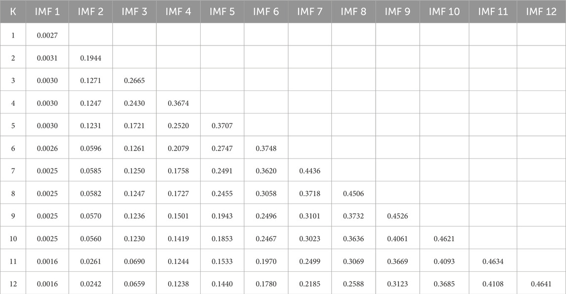
Table 2. Evaluation of the optimal number of components, with center frequencies.

A second complementary way of determining the optimal number of components is proposed by evaluating the correlation between the initial series data and the sum of the IMF components. Being an additive decomposition, the sum of the components results in the estimate of the initial data. Figure 3 shows the correlation between the normalized data of the zonal wind at Lima at 80.5 km height and the sum of its IMF components, for different values of $\mathrm{k}$. It is observed that when the series is decomposed from 11 components to more, the correlation values are approximate and almost constant. In this instance, both rules give similar results. Then it is determined that the number of components for this series is 12. Figure 4 shows the 12 components.

Figure 3

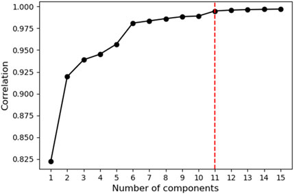
Figure 3. Correlations were calculated between the actual data and the sum of the components of zonal wind at Lima at 80.5 km height. When k = 11, the correlation appears to be constant.

Figure 4

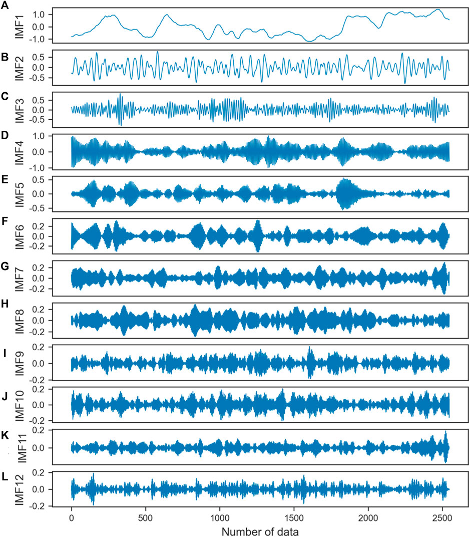
Figure 4. Components of the zonal wind at Lima at 80.5 km altitude. (A–L) show the 12 time series into which the original time series was decomposed.

2.5 Long short-term memory neural network

Long short-term memory neural network (LSTM) is an enhancement of the recurrent neural network (RNN), which has limitations such as gradient bursting and fading, lack of retention of historical information over time; and not distinguish between information that should be further processed and information that should be deleted. The LSTM network uses control gates that help solve the above problems. Within the LSTM block, there is a ring buffer and three gates named: input, forget, and output. Like RNNs, the LSTM network also has a hidden layer that processes the flow of information (Son and Jung, 2020).

Figure 5 shows the basic structure of the LSTM network. Its main features are the hidden layer ${\mathrm{h}}_{\mathrm{t}}$, the memory cell ${\mathrm{c}}_{\mathrm{t}}$ and the control gates (represented by the letters inside the circles). The first gate is the forgetting gate (letter f), which evaluates the elements to be purged from the cell state ${\mathrm{c}}_{\mathrm{t}-1}$ and outputs a resultant vector ${\mathrm{f}}_{\mathrm{t}}$. Then the cell state $\stackrel{\sim }{\mathrm{c}}$ is partially updated, processing the input ${\mathrm{x}}_{\mathrm{t}}$ and the previous hidden state ${\mathrm{h}}_{\mathrm{t}-1}$. The second gate is the input gate (letter i) which has a resultant vector ${\mathrm{i}}_{\mathrm{t}}$. This gate has the task of evaluating which information from the partial cell state $\stackrel{\sim }{{\mathrm{c}}_{\mathrm{t}}}$ serves to fully update the current time cell state ${\mathrm{c}}_{\mathrm{t}}$. Finally, there is the output gate (letter o) that controls the sending of the information from the current cell state ${\mathrm{c}}_{\mathrm{t}}$ to the new hidden state ${\mathrm{h}}_{\mathrm{t}}$ (Kratzert et al., 2018).

Figure 5

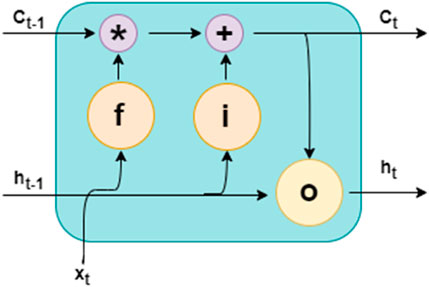
Figure 5. Neural network operation.

LSTM neural networks can be implemented using the function of the same name from the TensorFlow library in Python. Like the methodology proposed by Yang et al. (2023) a model with LSTM was performed for each IMF of each time series. For example, if a time series is determined to have 12 modal components, then 12 models with LSTM should be performed.

Before inputting the data to the neural network, the dimensions of the input and output data must be specified. In this case, we have experimented with a window of 56 consecutive data, corresponding to a period of 1 week. While the output data are 16 steps in the future, corresponding to 2-day records. Subsequently, hyperparameters such as dropout, number of layers and neurons, Adam optimizer, learning rate, and batch size were added (Mauricio et al., 2023).

Additionally, the Ridge regularization was introduced, which is a penalty applied to the loss function of the proposed model. This regularization was also used in the paper by Rosa et al. (2020), who performed a similar analysis with VMD and LSTM for the Piura River flow time series in Peru.

2.6 Optuna

Akiba et al. (2019) presented Optuna, a framework designed for hyperparameter optimization in the context of machine learning and deep learning. Optuna is based on a sequential optimization approach that uses the adaptive search tree-based optimization (TPE) algorithm to efficiently explore the hyperparameter space. Optuna is characterized by its ability to dynamically adapt to the hyperparameter space, allowing it to converge more quickly to optimal solutions. This is achieved by systematically exploring hyperparameter combinations, where decisions are based on previous observations to steer the search towards promising regions of the search space. The framework offers a simple user interface and seamless integration with machine learning and deep learning libraries, facilitating its use in a variety of applications. In addition, Optuna provides advanced tools such as experiment management and result visualization to facilitate the organization and analysis of optimization results. Optuna’s scalability stands out, as it is designed to handle large datasets and complex search spaces efficiently. This makes it suitable for both small-scale applications and large-scale research projects requiring complex model optimization. In summary, Optuna represents a significant breakthrough in automated hyperparameter optimization, offering a powerful and efficient solution for improving model performance. Its ability to dynamically adapt to the hyperparameter space and its seamless integration with popular libraries make it a valuable tool for researchers and practitioners in the field of machine learning.

Table 3 shows the set of hyperparameters used in this study. During optimization, Optuna provides tools that help to plot the loss curve that allows to evaluation of the learning performance of the models. Figure 6 shows the loss curves for the 12 components of the Piura zonal wind at 80.5 km altitude. Optuna has by default that the X-axis represents the number of epochs and the Y-axis represents the mean square error (MSE). However, since the data are normalized, the MSE values have no units of measurement.

Table 3

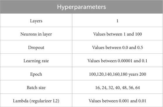
Table 3. Hyperparameter options.

Figure 6

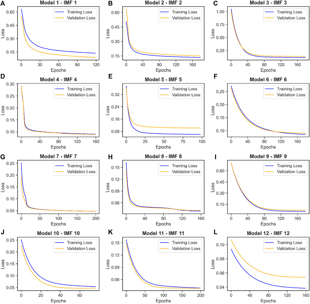
Figure 6. Training and validation loss curves for each component of the Piura zonal wind at 80.5 km altitude. (A–L) show that the training loss and validation loss curves decrease similarly in all cases.

2.7 Hybrid model

In summary of what has been explained in the previous paragraphs, the hybrid model applied in combines the VMD, LSTM and Optuna techniques (Figure 7). First, time series of normalized and complete data are obtained, which are then decomposed into their optimal components using the VMD algorithm. These components are reorganized into windows of 56 data, equivalent to 7 days. Each of these blocks is fed into an individual LSTM neural network, where the hyperparameters are optimized with Optuna. The output of each LSTM provides windows of 16 steps, corresponding to 2 days. Finally, the final prediction is the denormalization of the sum of the estimates calculated for each component.

Figure 7

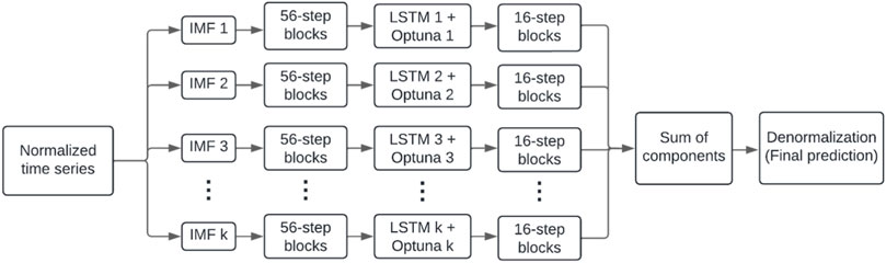
Figure 7. Diagram of the hybrid model.

2.8 Persistence model

Mauricio et al. (2023) used a persistence model that consists of the wind speed values of two previous days being repeated in the following 2 days. Through this model, a time series is reconstructed and compared with the hybrid model estimates. The intention is to demonstrate that the hybrid model is superior to the simplicity of the persistence model.

2.9 Model of dominant harmonics

The model of dominant harmonics was built from a sum of sinusoidal series with specified periods. In this model, the mean winds (an average of meridional wind and an average of zonal wind), as well as the amplitudes and phases of specific waves, were fitted using the least squares method, with a 7-day window. The selected periods correspond to the dominant wave periods obtained by the MLT climatology over the Peruvian sector (see Suclupe et al., 2023 for more details), which are 48, 24, 12, 8, and 6 h. Finally, the model was interpolated in a window of 2 days to compare it with the proposed hybrid model.

2.10 Evaluation of the hybrid model

Mauricio et al. (2023) reconstructed the time series by making predictions with a 16-step horizon. This approach involved the generation of sequential predictions of consecutive blocks of 16 steps within the time series. Specifically, predictions were initially applied to steps 1 through 16. Then, the process was repeated for steps 17 through 32, and so on, ensuring progressive coverage of the entire time series in 16-step intervals. This method allowed the evaluation of the predictive capability of the proposed model versus a 2-day persistence model, for multiple segments (training, validation, testing and February 2023 data), ensuring a complete evaluation of its performance over time. The metric used was RMSE and the proposed model was shown to be better.

In this paper, the RMSE was again used and the nonparametric Spearman correlation metric (r) was added. This coefficient is used to measure the strength and direction of the association between two variables, regardless of the distribution of the data. Assuming that the results show a mostly positive correlation, a correlation is considered to be very weak if its value is between 0.00 and 0.20, weak between 0.21 and 0.40, moderate between 0.41 and 0.60, strong between 0.61 and 0.80, and very strong between 0.81 and 1.00.

It was decided to evaluate the hybrid model in three stages. The first stage is related to evaluating that the estimates of the proposed model do not present overfitting and that it is superior to a simple model such as the persistence model. Similar to the analysis performed by Mauricio et al. (2023), the entire time series is estimated using 16-step predictions. That is, the 16-step blocks are joined and form a complete time series. It is confirmed that there is no overfitting when the calculated metrics of the hybrid model are similar in the training, validation and test data sets. On the other hand, it is confirmed that the hybrid model is better than the persistence model when the metrics of the hybrid model are better than those of the persistence model, using the same data sets.

The second stage was the step-by-step analysis. This method involves generating multiple predictions using continuous input windows. Predictions are made using the first 56 input steps, then the input window is shifted one position and new predictions are made using the next 56 steps, and so on. This process is repeated until the entire time series is covered. This approach facilitates obtaining vectors of estimates of all 1-steps, all 2-steps and so on up to the vector of 16-steps. This analysis was only performed on the test data, evaluating the predictive model performance at each time step.

In the third stage, the original data for the year 2023 (January to December) are available. The objective is to evaluate whether the hybrid model is better than the model of dominant harmonic for the year 2023. As in the first stage, a time series is reconstructed through the estimated consecutive blocks of 16 steps. It is evaluated which model is better, observing which one has better metrics.

3 Results

3.1 Data imputation

Table 4 shows the comparison of the descriptive statistics values before and after imputation for data previous to 2023. This was mentioned by Mauricio et al. (2023), but the values were not shown there.

Table 4

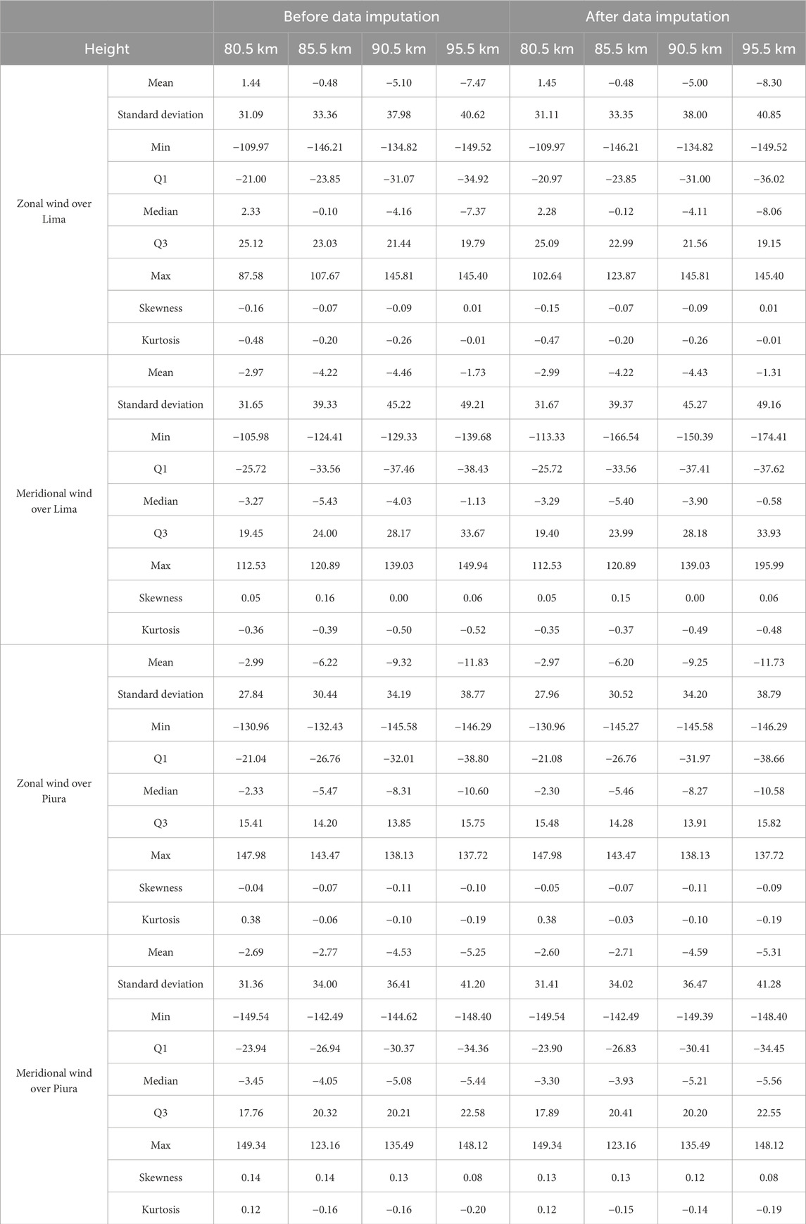
Table 4. Comparison of descriptive statistics before and after imputation.

In the second stage, the 2023 data were analyzed and a summary of the information on the amount of missing data was obtained. The result shows that the percentages were in the range between 8% and 15% (Table 5). As these percentages of missing data are higher than 6%, the time series was subdivided into blocks with lower percentages and the imputation process was replicated.

Table 5

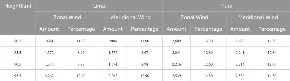
Table 5. Missing data in 2023.

3.2 VMD decomposition

The VMD decomposition analysis to determine the number of components of each time series is shown in Table 6. The values show convergence between 11 and 12 components. Above these values, the method is not optimal.

Table 6

Table 6. Number of IMF for each time series.

3.3 Evaluation of the hybrid model

3.3.1 Comparison with persistence model

The metrics in Tables 7, 8 are analyzed with the training, validation and test data sets for the Lima and Piura locations, respectively. The metrics show that the hybrid model is better than the persistence model in both locations.

Table 7

Table 7. Evaluation of the hybrid model for Lima data.

Table 8

Table 8. Evaluation of the hybrid model for Piura data.

In the case of Lima, the hybrid model has RMSE values that vary between 12.38 ${\mathrm{m}\mathrm{s}}^{-1}$ and 22.5 ${\mathrm{m}\mathrm{s}}^{-1}$, while the correlation values vary between 0.81 and 0.94. In comparison, the persistence model has higher RMSE with values that vary between 26.36 ${\mathrm{m}\mathrm{s}}^{-1}$ and 47.52 ${\mathrm{m}\mathrm{s}}^{-1}$, while the correlation values are lower and vary between 0.24 and 0.64.

In the case of Piura, the RMSE values vary between 10.79 ${\mathrm{m}\mathrm{s}}^{-1}$ and 27.04 ${\mathrm{m}\mathrm{s}}^{-1}$, while the correlation values vary between 0.67 and 0.93. In comparison, the persistence model has higher RMSE with values that vary between 29.01 ${\mathrm{m}\mathrm{s}}^{-1}$ and 43.78 ${\mathrm{m}\mathrm{s}}^{-1}$, while the correlation values are lower than 0.48.

In addition, the values of the hybrid model metrics in the three data sets (training, validation and test), do not have large differences. This is an indicator that the model does not have overfitting.

3.3.2 Step analysis

As noted in the methodology, this analysis was only performed on the test data set. The metrics calculated for each time step show an increase in RMSE (Figure 8) and a decrease in correlation (Figure 9). This indicates that within the windows of 16 prediction steps, the first steps fit better than the last steps.

Figure 8

Figure 8. RMSE values for each time step in Lima. (A) shows the RMSE values for the zonal wind. (B) shows the RMSE values for the meridional wind.

Figure 9

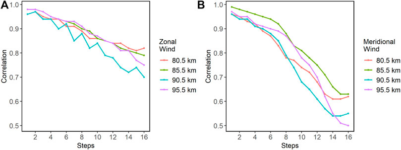
Figure 9. Correlation values for each time step in Piura. (A) shows the correlation values for the zonal wind. (B) shows the correlation values for the meridional wind.

In the case of Lima, the RMSE values increase from 6.46 ${\mathrm{m}\mathrm{s}}^{-1}$ to 30.84 ${\mathrm{m}\mathrm{s}}^{-1}$, while the correlation values decrease from 0.99 to 0.66. For example, the meridional wind at 85.5 km of altitude, has the best 1-step with an RMSE of 6.46 ${\mathrm{m}\mathrm{s}}^{-1}$ and a correlation of 0.99, while the 16-step has an RMSE of 23.05 and a correlation of 0.8.

In the case of Piura, the RMSE values increase from 6.04 ${\mathrm{m}\mathrm{s}}^{-1}$ to 30.41 ${\mathrm{m}\mathrm{s}}^{-1}$, while the correlation values decrease from 0.99 to 0.5. For example, the zonal wind at 85.5 km of altitude, has the best 1-step with an RMSE of 6.04 ${\mathrm{m}\mathrm{s}}^{-1}$ and a correlation of 0.98, while the 16-step has an RMSE of 17.42 ${\mathrm{m}\mathrm{s}}^{-1}$ and a correlation of 0.79.

3.3.3 Comparison with the model of dominant harmonics

The comparison of metrics between the hybrid model and the model of dominant harmonics with data from 2023 is shown in Table 9 for Lima and Table 10 for Piura.

Table 9

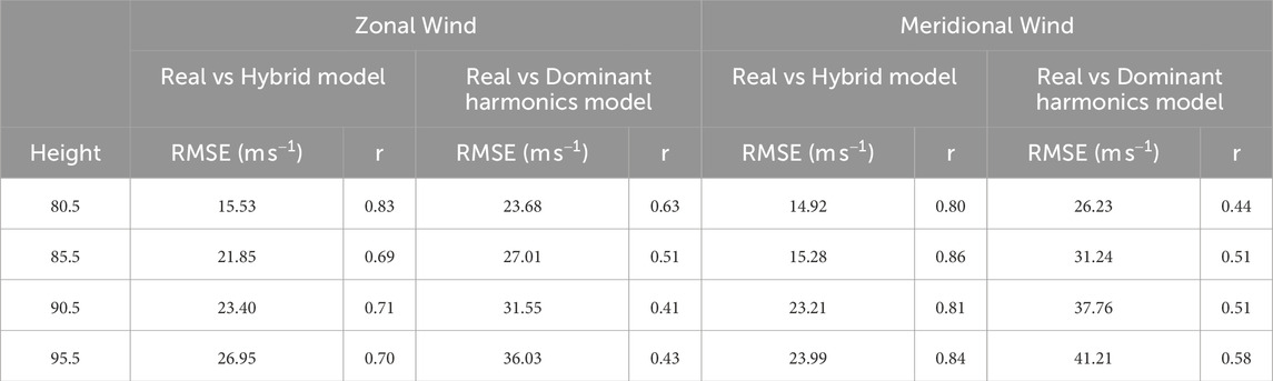
Table 9. Comparison metrics between the hybrid model and interpolation in 2023 (Lima).

Table 10

Table 10. Comparison metrics between the hybrid model and interpolation in 2023 (Piura).

In the case of Lima, the hybrid model has RMSE values ranging from 14.92 ${\mathrm{m}\mathrm{s}}^{-1}$ to 26.95 ${\mathrm{m}\mathrm{s}}^{-1}$, while the correlation values range from 0.69 to 0.86. The model of dominant harmonics has RMSE values ranging between 23.68 ${\mathrm{m}\mathrm{s}}^{-1}$ and 41.21 ${\mathrm{m}\mathrm{s}}^{-1}$, while correlation values vary between 0.41 and 0.63. Figure 10 shows the time series predictions of the zonal wind in Lima at 80.5 km altitude, made by both models, with their respective scatter diagrams. The hybrid model has an RMSE of 15.53 ${\mathrm{m}\mathrm{s}}^{-1}$ and a correlation of 0.83, while the model of dominant harmonics has an RMSE of 23.68 ${\mathrm{m}\mathrm{s}}^{-1}$ and a correlation of 0.63. It is observed that the hybrid model has a lower RMSE value and a higher correlation value. Additionally, in the scatter plot, the predictions of the hybrid model are better fitted to the data in Lima.

Figure 10

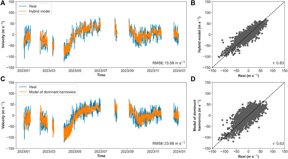
Figure 10. Comparison between the hybrid and dominant harmonics model estimates for the zonal wind at 80.5 km height in Lima in the year 2023. (A) shows the 2023 time series versus the hybrid model estimates. (B) shows the scatter plot of the 2023 data versus the hybrid model estimates. (C) shows the 2023 time series versus the model of dominant harmonic estimates. (D) shows the scatter plot of the 2023 data versus the model of dominant harmonic estimates.

In the case of Piura, the hybrid model has RMSE values ranging from 15.47 ${\mathrm{m}\mathrm{s}}^{-1}$ to 26.80 ${\mathrm{m}\mathrm{s}}^{-1}$, while the correlation values range from 0.55 to 0.80. The model of dominant harmonics has RMSE values ranging between 21.87 ${\mathrm{m}\mathrm{s}}^{-1}$ and 41.57 ${\mathrm{m}\mathrm{s}}^{-1}$, while correlation values vary between 0.26 and 0.5. Figure 11 shows the time series predictions of the meridional wind in Piura at 95.5 km altitude, made by both models, with their respective scatter diagrams. The hybrid model has an RMSE of 19.34 ${\mathrm{m}\mathrm{s}}^{-1}$ and a correlation of 0.80, while the model of dominant harmonics has an RMSE of 41.57 ${\mathrm{m}\mathrm{s}}^{-1}$ and a correlation of 0.40. Similar to the results for Lima, the hybrid model is found to have a lower RMSE, a higher correlation, and less dispersion with respect to the model of dominant harmonics. Also, their scatter plot indicates that the predictions of the hybrid model better fit the 2023 data collected in Piura.

Figure 11

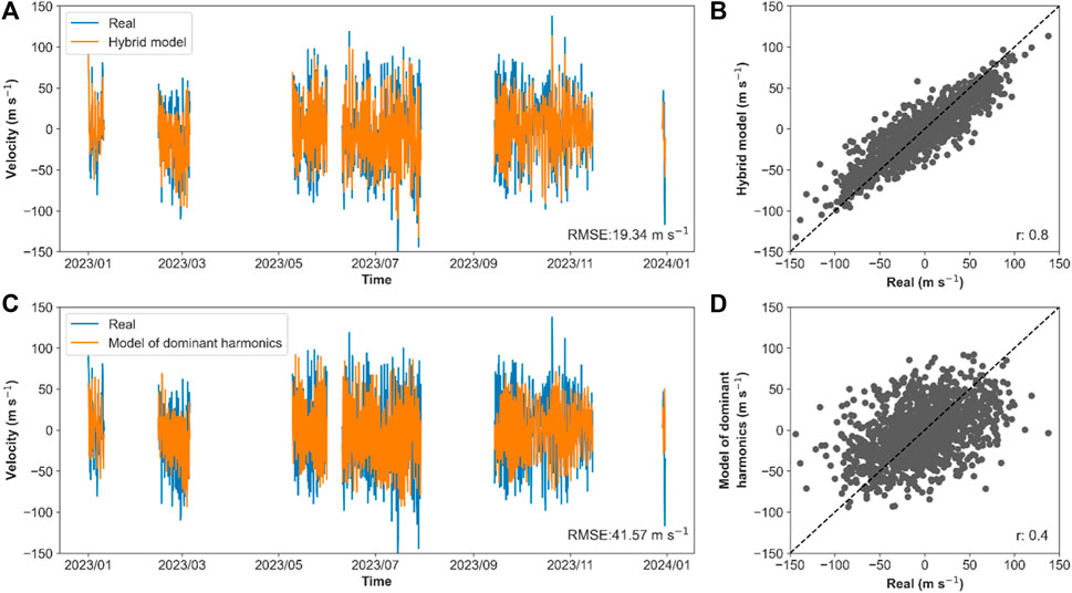
Figure 11. Comparison between the estimates made by the hybrid model and the model of dominant harmonics, for the meridional wind at 95.5 km height in Piura in the year 2023. (A) shows the 2023 time series versus the hybrid model estimates. (B) shows the scatter plot of the 2023 data versus the hybrid model estimates. (C) shows the 2023 time series versus the model of dominant harmonic estimates. (D) shows the scatter plot of the 2023 data versus the model of dominant harmonic estimates.

4 Discussion and conclusions

The imputation of missing data for 2023 was performed under the assumption that the percentage limit of missing data is 6%. However, it is necessary to have sufficient data to allow this analysis to be carried out. If there are only a few data points available, the distribution may not be symmetrical because of certain values that dominate that period. In addition, it is essential to have at least 72 continuous data to be able to make predictions and calculate metrics (56 input data points and 16 output data points).

In determining the number of components of the time series, convergence is observed between the values of 11 and 12 components. Exceeding these values can lead to poor estimates of the original series. Having these limits defined helps to avoid making unnecessary models of the components, avoiding execution times and the use of computational resources. Additionally, for future research, associations between these components and other meteorological time measurements could be evaluated.

During the modeling phase, the inclusion of the regularizer (L2) resulted in a marked improvement in the visualization of the loss curves for both the training and validation sets, which helped to avoid overfitting the models. As for Optuna, only 30 search iterations per component were performed. Although a more exhaustive search could provide even more accurate estimates, the complexity of the model, with 11 or 12 components, implies lengthy processing and higher consumption of computational resources. Similarly, increasing the number of epochs and the number of layers could improve the search, but the processing would be much longer.

On the other hand, the amount of data used in the modeling corresponds to a period of approximately 1 year. Since the SIMONe radars are still active, this amount of data could increase. This would allow a better recognition of temporal patterns to make better estimates.

As for the input and output data, there is also a possibility for improvement. Two paths can be followed. First, keep the same input data window to predict fewer output steps. For example, one can predict 8 steps corresponding to 1 day of records. Second, one can increase the size of the input window to 112, corresponding to 2 weeks of records, while keeping the 16 output steps.

Detailed analysis of the predictions reveals a significant deterioration in the metrics towards the final steps. This observation justifies the exploration of predictions with a shorter time horizon than the 16 steps, keeping the same input window. When reconstructing the time series using blocks of 16 estimates, it was observed that certain parts of these series did not correctly match the actual data. This mismatch was mainly attributed to the low precision of the estimates for the last steps. Despite the challenges, the proposed hybrid model has shown better performance than the model of dominant harmonics when comparing the predictions to the actual 2023 data using RMSE and correlation metrics. In other words, the hybrid model more accurately matched the actual data. Possibly, the hybrid model can capture other significant waves of planetary scale and mesoscale. This speculation will be evaluated in future works.

Data availability statement

The raw data supporting the conclusions of this article will be made available by the authors, without undue reservation.

Author contributions

CM: Writing–original draft, Writing–review and editing. JS: Writing–original draft, Writing–review and editing. MM: Writing–review and editing. CL: Writing–review and editing. KK: Writing–review and editing. DS: Writing–review and editing. RR: Writing–review and editing.

Funding

The author(s) declare financial support was received for the research, authorship, and/or publication of this article. This work was supported and financed by PROCIENCIA (Peru), under contract No 075-2021-FONDECYT.

Acknowledgments

We also wish to thank the Leibniz Institute of Atmospheric Physics for providing MLT winds from SIMONe radar networks. We also thank Jorge Chau for his suggestions that contributed to the development of this work. Additionally, we acknowledge the collaboration of the Estación Ramón Mujica of the Universidad of Piura and the Radio Observatorio de Jicamarca of the Instituto Geofísico del Perú for providing support in the operation of the SIMONe radar system. Finally, we extend our gratitude to the Pontificia Universidad Católica del Perú y la Universidad Nacional Agraria La Molina for guiding the methodology of data processing.

Conflict of interest

The authors declare that the research was conducted in the absence of any commercial or financial relationships that could be construed as a potential conflict of interest.

Publisher’s note

All claims expressed in this article are solely those of the authors and do not necessarily represent those of their affiliated organizations, or those of the publisher, the editors and the reviewers. Any product that may be evaluated in this article, or claim that may be made by its manufacturer, is not guaranteed or endorsed by the publisher.

References

Akiba, T., Sano, S., Yanase, T., Ohta, T., and Koyama, M. (2019). “Optuna: a next-generation hyperparameter optimization framework,” in In Proceedings of the ACM SIGKDD International Conference on Knowledge Discovery and Data Mining (Association for Computing Machinery), 2623–2631.

CrossRef Full Text | Google Scholar

Ali, M., Khan, A., and Rehman, N. (2018). Hybrid multiscale wind speed forecasting based on variational mode decomposition. Int. Trans. Electr. Energy Syst. 28 (1), e2466. doi:10.1002/etep.2466

CrossRef Full Text | Google Scholar

Carvalho, V. R., Moraes, M. F. D., Braga, A. P., and Mendes, E. M. A. M. (2020). Evaluating five different adaptive decomposition methods for EEG signal seizure detection and classification. Biomed. Signal Process. Control 62, 102073. doi:10.1016/j.bspc.2020.102073

CrossRef Full Text | Google Scholar

Chau, J. L., Urco, J. M., Vierinen, J., Harding, B. J., Clahsen, M., Pfeffer, N., et al. (2021). Multistatic specular meteor radar network in Peru: system description and initial results. Earth Space Sci. 8 (1), 1–22. doi:10.1029/2020EA001293

CrossRef Full Text | Google Scholar

Conte, J. F., Chau, J. L., Yiǧit, E., Suclupe, J., and Rodríguez, R. (2024). Investigation of mesosphere and lower thermosphere dynamics over central and northern Peru using SIMONe systems. J. Atmos. Sci. 81 (1), 93–104. doi:10.1175/JAS-D-23-0030.1

CrossRef Full Text | Google Scholar

Dhadly, M., Sassi, F., Emmert, J., Drob, D., Conde, M., Wu, Q., et al. (2023). Neutral winds from mesosphere to thermosphere—past, present, and future outlook. Front. Astronomy Space Sci. 9. doi:10.3389/fspas.2022.1050586

CrossRef Full Text | Google Scholar

Dragomiretskiy, K., and Zosso, D. (2014). Variational mode decomposition. IEEE Trans. Signal Process. 62 (3), 531–544. doi:10.1109/TSP.2013.2288675

CrossRef Full Text | Google Scholar

Emmert, J. T., Drob, D. P., Picone, J. M., Siskind, D. E., Jones, M., Mlynczak, M. G., et al. (2021). NRLMSIS 2.0: a whole-atmosphere empirical model of temperature and neutral species densities. Earth Space Sci. 8 (3). doi:10.1029/2020EA001321

CrossRef Full Text | Google Scholar

Forbes, J. M. (1995). Tidal and planetary waves’. In. Geophysical monograph series, edited by R. M. Johnson, and T. L. Killeen, 67–87. Washington, D. C.: American Geophysical Union. doi:10.1029/GM087p0067

CrossRef Full Text | Google Scholar

Gan, M., Pan, H., Chen, Y., and Pan, S. (2021). Application of the variational mode decomposition (VMD) method to river tides. Estuar. Coast. Shelf Sci. 261, 107570. doi:10.1016/j.ecss.2021.107570

CrossRef Full Text | Google Scholar

Gasperini, F., Jones, M. A., Harding, B. J., and Immel, T. J. (2023). Direct observational evidence of altered mesosphere lower thermosphere mean circulation from a major sudden stratospheric warming. Geophys. Res. Lett. 50 (7). doi:10.1029/2022GL102579

CrossRef Full Text | Google Scholar

Hanifi, S., Lotfian, S., Zare-Behtash, H., and Cammarano, A. (2022). Offshore wind power forecasting—a new hyperparameter optimisation algorithm for deep learning models. Energies 15 (19), 6919. doi:10.3390/en15196919

CrossRef Full Text | Google Scholar

Hussin, N. H., Yusof, F., Jamaludin, A. R., and Norrulashikin, S. M. (2021). Forecasting wind speed in peninsular Malaysia: an application of arima and arima-garch models. Pertanika J. Sci. Technol. 29 (1), 31–58. doi:10.47836/pjst.29.1.02

CrossRef Full Text | Google Scholar

Immel, T. J., Sagawa, E., England, S. L., Henderson, S. B., Hagan, M. E., Mende, S. B., et al. (2006). Control of equatorial ionospheric morphology by atmospheric tides. Geophys. Res. Lett. 33 (15). doi:10.1029/2006GL026161

CrossRef Full Text | Google Scholar

Kratzert, F., Klotz, D., Brenner, C., Schulz, K., and Herrnegger, M. (2018). Rainfall-runoff modelling using Long short-term memory (LSTM) networks. Hydrology Earth Syst. Sci. 22 (11), 6005–6022. doi:10.5194/hess-22-6005-2018

CrossRef Full Text | Google Scholar

Liu, H., Yamazaki, Y., and Lei, J. (2021). Day-to-Day variability of the thermosphere and ionosphere. Geophys. Monogr. Ser., 275–300. doi:10.1002/9781119815631.ch15

CrossRef Full Text | Google Scholar

Liu, H.Li, Bardeen, C. G., Foster, B. T., Lauritzen, P., Liu, J., Lu, G., et al. (2018). Development and validation of the whole atmosphere community climate model with thermosphere and ionosphere extension (WACCM-X 2.0). J. Adv. Model. Earth Syst. 10 (2), 381–402. doi:10.1002/2017MS001232

CrossRef Full Text | Google Scholar

Mauricio, C., Suclupe, J., Milla, M., López de Castilla, C., Karim, K., Rodriguez, R., et al. (2023). “Short-term prediction of wind speed in the mesosphere and lower thermosphere over Peru’s coastal north and central,” in 2023 IEEE CHILEAN Conference on Electrical, Electronics Engineering, Information and Communication Technologies (CHILECON), Valdivia, Chile, 05-07 December 2023 (IEEE), 1–6.

CrossRef Full Text | Google Scholar

McCormack, J. P., Coy, L., and Singer, W. (2014). Intraseasonal and interannual variability of the quasi 2 Day wave in the northern hemisphere summer mesosphere. J. Geophys. Res. Atmos. 119 (6), 2928–2946. doi:10.1002/2013JD020199

CrossRef Full Text | Google Scholar

Piani, C., Durran, D., Alexander, M. J., and Holton, J. R. (2000). A numerical study of three-dimensional gravity waves triggered by deep tropical convection and their role in the dynamics of the QBO. J. Atmos. Sci. 57 (22), 3689–3702. doi:10.1175/1520-0469(2000)057<3689:ANSOTD>2.0.CO;2

CrossRef Full Text | Google Scholar

Pigott, T. D. (2001). A review of methods for missing data. Educ. Res. Eval. 7 (4), 353–383. doi:10.1076/edre.7.4.353.8937

CrossRef Full Text | Google Scholar

Rosa, L., La, G., and Sanchez, I. (2020). “Hybrid models based on mode decomposition and recurrent neural networks for streamflow forecasting in the chira river in Peru,” in Proceedings of the 2020 IEEE Engineering International Research Conference, EIRCON 2020, Lima, Peru, 21-23 October 2020 (Institute of Electrical and Electronics Engineers Inc).

Google Scholar

Schneider, T. (2001). Analysis of incomplete climate data: estimation of mean values and covariance matrices and imputation of missing values. J. Clim. 14 (5), 853–871. doi:10.1175/1520-0442(2001)014<0853:AOICDE>2.0.CO;2

CrossRef Full Text | Google Scholar

Son, N., and Jung, M. (2020). Analysis of meteorological factor multivariate models for medium- and long-term photovoltaic solar power forecasting using Long short-term memory. Appl. Sci. 11 (1), 316. doi:10.3390/app11010316

CrossRef Full Text | Google Scholar

Staszak, T., Strelnikov, B., Latteck, R., Renkwitz, T., Friedrich, M., Baumgarten, G., et al. (2021). Turbulence generated small-scale structures as PMWE formation mechanism: results from a rocket campaign. J. Atmos. Solar-Terrestrial Phys. 217, 105559. doi:10.1016/j.jastp.2021.105559

CrossRef Full Text | Google Scholar

Suclupe, J., Chau, J. L., Federico Conte, J., Milla, M., Pedatella, N. M., and Kuyeng, K. (2023). Climatology of mesosphere and lower thermosphere diurnal tides over Jicamarca (12^ºS, 77 ^ºW): observations and simulations. Earth, Planets Space. Springer Sci. Bus. Media Deutschl. GmbH 75, 186. doi:10.1186/s40623-023-01935-z

CrossRef Full Text | Google Scholar

Vincent, R. A. (2015). The dynamics of the mesosphere and lower thermosphere: a brief review. Prog. Earth Planet. Sci. 2 (1), 4. doi:10.1186/s40645-015-0035-8

CrossRef Full Text | Google Scholar

Yang, S., Yang, H., Li, N., and Ding, Z. (2023). Short-term prediction of 80–88 Km wind speed in near space based on VMD–PSO–LSTM. Atmosphere 14 (2), 315. doi:10.3390/atmos14020315

CrossRef Full Text | Google Scholar