Scalar field solutions and energy bounds for modeling spatial oscillations in Schwarzschild black holes based on the Regge–Wheeler equation

This text discusses the behavior of solutions and the energy stability within Schwarzschild spacetimes, with a particular emphasis on the behavior of massless scalar fields under the influence of a non-rotating and spherically symmetric black hole. The stability of solutions in the proximity of the event horizon of black holes in general relativity remains an open question, especially given the difficulties introduced by minor perturbations that may resemble Kerr solutions. To address this, this work explores a simplified model, including massless scalar fields, to better understand perturbation behaviors around black holes under the Schwarzschild approach. We depart from Richard Price’s work in connection with how scalar, electromagnetic, and gravitational fields behave. The tortoise coordinate transformation is considered to set the stage for numerical solutions to the wave equations. Afterward, we explore energy estimates, which are used to gauge stability and wave behavior over time. Our analysis reveals that the time evolution of the energy does not exceed twice its initial value. Further and under the assumption of initial conditions in $L^2-$spaces, we obtain an exponential decreasing behavior in the energy time evolution. A question to continue exploring is how perturbations in $L^2$ in the initial conditions that introduce Kerr solutions as a second-order effect in the linearized equations perturb this obtained exponential decay.

1 Introduction and problem formulation

The study of the formation and evolution of black holes and the physical processes occurring in their vicinity is an important area of contemporary research. As an example, we can cite the importance of understanding the behavior of primordial black holes (PBHs), which constitute a research area of notable impact for describing dark matter interactions (De Luca et al., 2020). A major unresolved challenge in general relativity is the nonlinear stability of Schwarzschild solutions, which is complicated by the fact that small perturbations in the initial data can inadvertently include Kerr solution characteristics. The presence of an ergosphere further complicates deriving meaningful energy estimates for perturbed Schwarzschild solutions, particularly for rotating black holes or those that are slightly rotating due to perturbations, for example. One relevant option to characterize black holes is based on the study of their quasinormal modes (QNMs) (see (Kokkotas and Schmidt (1999) and Nollert (1999) for detailed definitions), the damped oscillations of black hole spacetimes, which can provide descriptions when spacetimes are slightly deformed from the Kerr solution (Zimmerman et al., 2015). For Schwarzschild black holes immersed in electromagnetic fields, the perturbation equations can be transformed into confluent Heun’s equations, enabling both analytical and numerical analyses of QNMs (Övgün et al., 2018). Greybody factors (GFs) and QNMs are also relevant in the understanding of the radiation spectra emitted by black holes, particularly under the forms of gravitational waves (Sakallı and Kanzi, 2022). Additionally, the relationship between black hole entropy, spin, and QNMs, particularly when considering non-extensive entropies, provides microstates and thermodynamic properties of black holes, with significant modifications for micro black holes (Martínez-Merino and Sabido, 2022).

It is prudent to consider a simplified problem, given the complexities involved in proving the full stability of Schwarzschild solutions. One approach is to investigate the linearized problem, focusing on the stability of the zero solutions. Another simplification can be achieved by considering a simpler linear field theory, such as the linear scalar field. An additional simplification involves restricting the analysis to spherically symmetric cases (Rendall, 2008). In the study of linear massless scalar fields within the context of Schwarzschild spacetime, the Regge–Wheeler equation provides a framework for analyzing perturbations around a Schwarzschild black hole (Regge and Wheeler, 1957). Price (1972) used this framework to derive the long-term behavior of these perturbations. Price’s work is particularly relevant for understanding how scalar fields, such as electromagnetic and gravitational fields, behave in the vicinity of a black hole, which may lead to phenomena such as wave scattering and the late-time tail behavior of these fields.

In a Schwarzschild spacetime describing the gravitational field outside a spherically symmetric, non-rotating, uncharged mass, a massless scalar field $\mu$ is well known to obey the Klein–Gordon equation for a massless particle:

$\square \mu =0$

Here, $\square$ denotes the d’Alembertian operator in generally curved spacetime.

Price’s investigations revealed that outside a black hole, perturbations from a massless field decay over time, but interestingly, they do so in a manner that leaves a “tail” of radiation (Price, 1972; Rendall, 2008). This tail is not an immediate cutoff but a slow, power-law decay of the field’s amplitude over time. Specifically, Price showed that after the initial wavefront passes, the field decays as $t^{-(2l_0+3)}$, where $t$ is time, and $l_0$ is the multipole moment (or angular quantum number) of the perturbation. This result implies that the gravitational influence of a black hole extends beyond its immediate vicinity, affecting the propagation of scalar fields over long periods.

In this work, we will make use of the transformation to the tortoise coordinate $r^{*}$ and the introduction of a scaled wave function $\psi =r\varphi$, where $\varphi$, the original wave function, describes the scalar field. This framework simplifies the analysis of wave equations in Schwarzschild spacetime by flattening the potential barrier experienced by waves as they approach the event horizon (Rendall, 2008).

Let us introduce some basic concepts to derive the main equation to be discussed in this work, typically referred to as the Regge–Wheeler Equation 3. Consider the scalar field $\varphi$ in spherical coordinates $(t,r,\theta ,\varphi )$ and the spherical harmonics with indices $l$ and $m$, $Y_{lm}(\theta ,\varphi )$. Using the tortoise coordinate (as it will be introduced later) along with a radial symmetry condition leads to considering the problem’s rotational invariance (Rendall, 2008; Zhao et al., 2022). Then, it holds that

$\mu \left(t,r,\theta ,\varphi \right)={\displaystyle \sum _{l=0}^{\infty }}{\displaystyle \sum _{m=-l}^l}{\psi }_{lm}\left(t,r\right)Y_{lm}\left(\theta ,\varphi \right).$

Here, ${\psi }_{lm}(t,r)$ are the radial and time-dependent components of the field. For the Schwarzschild metric, the determinant $g$ is $-r^2\sin \theta$, and the inverse metric components $g^{\mu \nu }$ are

$\begin{array}{ll}\hfill g^{tt}& =-{\left(1-\frac{2M}{r}\right)}^{-1},g^{rr}=1-\frac{2M}{r},g^{\theta \theta }=\frac{1}{r^2},\hfill \\ \hfill g^{\varphi \varphi }& =\frac{1}{r^2{\sin }^2\theta }.\hfill \end{array}$

The massless Klein–Gordon equation, $\square \mu =0$, in this metric becomes

$\begin{array}{ll}\hfill & -{\left(1-\frac{2M}{r}\right)}^{-1}{\partial }_t^2\mu +\frac{1}{r^2}{\partial }_r\left(r^2\left(1-\frac{2M}{r}\right){\partial }_r\mu \right)\hfill \\ \hfill & +\frac{1}{r^2}{\mathrm{\Delta }}_{\mathrm{\Omega }}\mu =0,\hfill \end{array}$

where ${\mathrm{\Delta }}_{\mathrm{\Omega }}$ is the angular part of the Laplacian in spherical coordinates:

${\mathrm{\Delta }}_{\mathrm{\Omega }}\mu =\frac{1}{\sin \theta }{\partial }_{\theta }\left(\sin \theta {\partial }_{\theta }\mu \right)+\frac{1}{{\sin }^2\theta }{\partial }_{\varphi }^2\mu .$

Substituting the expansion of $\mu$,

$\mu \left(t,r,\theta ,\varphi \right)={\displaystyle \sum _{l=0}^{\infty }}{\displaystyle \sum _{m=-l}^l}{\psi }_{lm}\left(t,r\right)Y_{lm}\left(\theta ,\varphi \right),$

we obtain

$\begin{array}{ll}\hfill & -{\left(1-\frac{2M}{r}\right)}^{-1}{\displaystyle \sum _{l,m}}{\ddot{\psi }}_{lm}\left(t,r\right)Y_{lm}\hfill \\ \hfill & +\frac{1}{r^2}{\partial }_r\left(r^2\left(1-\frac{2M}{r}\right){\partial }_r{\displaystyle \sum _{l,m}}{\psi }_{lm}{Y}_{lm}\right)\hfill \\ \hfill & +\frac{1}{r^2}{\displaystyle \sum _{l,m}}{\psi }_{lm}{\mathrm{\Delta }}_{\mathrm{\Omega }}{Y}_{lm}=0.\hfill \end{array}$

Using the property of spherical harmonics,

${\mathrm{\Delta }}_{\mathrm{\Omega }}{Y}_{lm}=-l\left(l+1\right)Y_{lm},$

we separate the angular and radial parts:

$\begin{array}{ll}\hfill & -{\left(1-\frac{2M}{r}\right)}^{-1}{\ddot{\psi }}_{lm}+\frac{1}{r^2}{\partial }_r\left(r^2\left(1-\frac{2M}{r}\right){\partial }_r{\psi }_{lm}\right)\hfill \\ \hfill & -\frac{l\left(l+1\right)}{r^2}{\psi }_{lm}=0.\hfill \end{array}$

Introducing the tortoise coordinate $r_{\ast }$ as

$\frac{d{r}^{*}}{dr}={\left(1-\frac{2M}{r}\right)}^{-1},(1)$

the radial part of the Klein–Gordon equation can be written as

$\left(\frac{{\partial }^2}{\partial t^2}-\frac{{\partial }^2}{\partial {\left(r^{*}\right)}^2}-F_l\left(r^{*}\right)\right){\psi }_{lm}\left(t,r^{*}\right)=0,(2)$

This decomposition leads to a radial wave equation where $F_l(r^{*})$ appears as the effective potential (this can be further observed in our results given in Figure 2) and adopts the following expression:

$F_l\left(r^{*}\right)=\left(1-\frac{2M}{r}\right)\left(\frac{l\left(l+1\right)}{r^2}+\frac{2M}{r^3}\right),$

and the spherical harmonics $Y_{lm}(\theta ,\varphi )$ are given by

$Y_{lm}\left(\theta ,\varphi \right)={\left(-1\right)}^m\sqrt{\frac{\left(2l+1\right)}{4\pi }\frac{\left(l-m\right)!}{\left(l+m\right)!}}{P}_{lm}\left(\cos \theta \right)e^{im\varphi },$

where $P_{lm}(\cos \theta )$ are the associated Legendre polynomials. The indices $l$ and $m$ are integers with $l\ge 0$ and $-l\le m\le l$. The index $l$ determines the total angular momentum, while $m$ determines the projection of the angular momentum on the z-axis.

Upon integration in the Equation (1), the tortoise coordinate $r^{*}$ can be rewritten as

$r^{*}=r+2M\log \left(\frac{r-2M}{2M}\right)$

This coordinate stretches the region near the event horizon at $r=2M$ for a Schwarzschild black hole of mass $M$. The tortoise coordinate is well known to facilitate the analysis of fields near and at the event horizon. Here, $r$ is the usual radial coordinate in Schwarzschild spacetime.

We now introduce some relevant objectives of our work. We aim to study the QNMs based on Equation 2 with the potential F_l(r^*), in line with Zhao et al. (2022) and Balart et al. (2023) and, more particularly, the behavior of such QNMs with respect to the tortoise coordinate. The QNMs represent solutions to the wave equation that behave like damped oscillations that decay over time, emitting gravitational waves in the process. Hence, and to start our analysis with more familiar assessments, we assume that the QNMs are given based on an expression of the form: $\psi (r^{*},t)=e^{-i\omega t}\mathrm{\Psi }(r^{*})$ and this expression can be written for all $m,l$ so we omit the sub-index for simplification in notation. In addition, we consider a description of the field subjected to the potential F_l(r^*). Then, substituting into the wave Equation 2 and dividing by $e^{-i\omega t}$ yields

$-{\omega }^2\mathrm{\Psi }\left(r^{*}\right)-\frac{{\partial }^2\mathrm{\Psi }}{\partial {\left(r^{*}\right)}^2}=F_l\left(r^{*}\right)\mathrm{\Psi }\left(r^{*}\right).$

Rearranging terms,

$\frac{{\partial }^2\mathrm{\Psi }}{\partial {\left(r^{*}\right)}^2}+\left[{\omega }^2-F_l\left(r^{*}\right)\right]\mathrm{\Psi }\left(r^{*}\right)=0.(3)$

This equation can be seen as analogous to the time-independent Schrödinger equation,

$-\frac{{\hslash }^2}{2m_p}\frac{{\partial }^2\mathrm{\Psi }}{\partial x^2}+V\left(x\right)\mathrm{\Psi }=E\mathrm{\Psi },$

where the term $\left[{\omega }^2-F_l(r^{*})\right]$ is analogous to the energy $E$ (minus the potential energy $V(x)$) in the Schrödinger equation. Hence, we may consider the theory of potentials available to resolve the Schrödinger-type equations. In the first step, we will provide some numerical solutions for this last equation to describe the behavior of waves with regard to the tortoise coordinate, and afterward, we provide energy estimates to describe the time evolution.

2 Methodology

In the first step, we introduce a numerical implementation to describe the behavior of the wave function described by the radial wave in (Equation 3) along with the effective potential $F_l(r^{*})$. The transformation from the Schwarzschild radial coordinate $r$ to the tortoise coordinate $r^{*}$ is given by expression (5) and provides the non-invertibility of this transformation. Analytically, numerical methods are required to back-calculate $r$ from $r^{*}$.

We note that the numerical solutions were obtained using well-established numerical methods, specifically Python’s textttscipy.integrate.solve_ivp function with the solvers “BDF” (Implicit multi-step method) and “LSODA” (that switches between the Adams and BDF methods). The initial range for $r^{*}$ is selected to ensure that the execution of the routines provides plausible solutions within the requested global error tolerance fixed at $10^{-3}$. The numerical process includes continuously validating the numerical solution against expected behaviors and refining the integration parameters to achieve convergence and accuracy.

In the second step, we combine analytical and numerical methods to derive energy estimates for scalar field perturbations in the context of a Schwarzschild non-rotating black hole. Such energy estimates are formulated using the integral of the energy density over the tortoise coordinate, and we employ Poincaré’s inequality to control the energy estimates. In addition, we introduce numerical simulations to confirm the theoretical predictions and to show that the energy decays over time following an exponential law provided that the initial conditions belong to $L^2$ space.

3 Numerical solutions

The numerical solutions illustrated in the graphs in Figure 1 represent the solutions to Equation 2 in the vicinity of the horizon $r\sim 2M$. These solutions were assumed to have the form $\psi (r^{*},t)=e^{-i\omega t}\mathrm{\Psi }(r^{*})$ and to be far from the horizon for increased values of $r^{*}$. For our purposes, we consider a fixed time $t=t_0=1.0$. Near the horizon $(r\sim 2M)$, the potential $V(r^{*})$ becomes very small, and the wave equation simplifies to a free wave equation. In addition and in this particular region (given for the coordinate $r^{*}$ going to negative values), Figure 1 allows us to observe the diverging behavior for a black hole mass of 10 times the solar mass and for different values of angular momentum number $l$. Indeed, the behavior of $\psi (r^{*})$ in this region is dominated by oscillatory modes (refer to Mamani et al. (2022) for additional discussions). Notably, the oscillatory nature is consistent with the expected QNMs behavior, where the modes oscillate but in the time domain (refer again to Keir (2020)). Note that the number $l$ has a significant impact on the transmission and reflection coefficients for wave scattering by the black hole (refer to Futterman et al. (1988) for additional insights), and this may lead to potential avenues for extracting physical information from observational data (Sathyaprakash and Schutz, 2009), a relevant issue in observational astronomy (see Virtanen et al. (2020)).

Figure 1

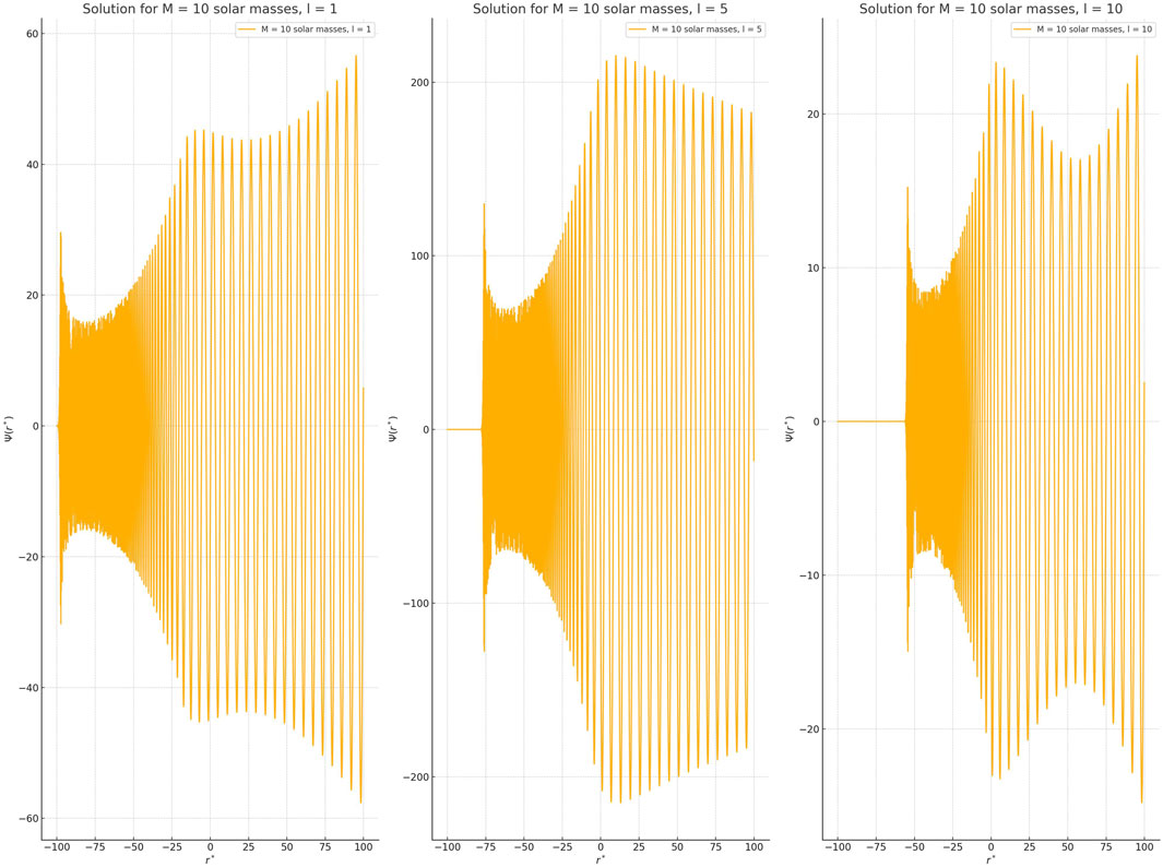
Figure 1. Real part of the wave functions $\psi (r^{*})$ as a function of the tortoise coordinate $r^{*}$ for a Schwarzschild black hole with mass $M=10$ solar masses, for different angular momentum quantum numbers $l$. The left panel shows $l=1$, the middle panel shows $l=5$, and the right panel shows $l=10$. The exponential divergence near the horizon (left negative values in $r^{*}$) increases oscillation complexity for higher $l$ values.

Based on the provided Figure 1, we can observe an exponentially diverging asymptotic behavior of the wave functions near the horizon for different values of the angular momentum quantum number $l$. As $r^{*}$ approaches large negative values, the wave functions $\mathrm{\Psi }(r^{*})$ in all three panels show an exponential divergence. This behavior is more pronounced with oscillations superimposed on the exponential growth. This exponential divergence is a characteristic feature near the event horizon and aligns with previous studies (see Zhao et al. (2022)). For small $l$ values (left panel), the exponential divergence starts relatively smoothly, with clear oscillations. As $l$ increases (middle and right panels), the oscillations become more rapid, and the exponential growth becomes more abrupt. Additionally, we observe a form of amplitude modulation in the wave functions, which is considered to be a result of the interference between different modes. As Berti et al. (2009) explain, the QNMs of black holes are not single-frequency oscillations but rather a spectrum of modes with different complex frequencies. When these modes interfere, they can produce beat-like patterns in the wave functions. This interference leads to the observed amplitude modulation, where the envelope of the wave function oscillations varies in a regular pattern. However, there is a key point: throughout the numerical resolution, the value of the frequency $\omega$ was fixed to a constant value in the term $e^{-i\omega t}$. Therefore, it is important to mention that the modulations in Figure 1 are due to the spatial modulation effect, not the temporal modulation attributed to temporal propagation. In this regard, we highlight that in conducting numerical analyses to understand the effect of oscillations with respect to the tortoise coordinate, it has been necessary to consider certain values for the frequencies of the QNMs that appear in the temporal phase of the solution $\psi (r^{*},t)=e^{-i\omega t}\mathrm{\Psi }(r^{*})$. For this purpose, different values compatible with the conditions given in [Fig. 5 ref (Berti et al., 2009)] have been considered. Furthermore, the observed behavior shown in Figure 1 has been tested for a wide range of $\omega$ values, exhibiting behaviors similar to the ones represented in the mentioned figure.

In addition, we should note that Zhao et al. (2022) provided graphical solutions in this direction, but certain other issues (like additional wave behavior for different values of $m,l$) were not contemplated, thus motivating us to include our analysis and to discuss further the implications. In addition, Keir (2020) concluded the existence of sublogarithmic time decay rates in the quasimodes for two-charge geometries, but there is no direct result to consider for the evolution with a radial coordinate and even further based on the tortoise coordinate.

4 Energy estimates

In the context of a Schwarzschild non-rotating black hole (with no ergoregion, or, if experienced, the ergoregion is considered as a second-order negligible term in our linear equations), making energy estimates is feasible both near the event horizon and far from it by utilizing the tortoise coordinate $r^{*}$. The Schwarzschild metric admits a static Killing vector field ${\partial }_t$ that remains time-like everywhere outside the event horizon. The effective potential $F_l(r^{*})$ derived from the Schwarzschild metric diminishes at large distances, simplifying the wave equation to a free wave equation, which allows the introduction of energy estimates. In addition, we shall note that the integration of the energy density over a large volume provides estimates of the total energy in the scalar field perturbation, applicable both in the strong regime for $r\sim 2M+ϵ$ (where $ϵ$ is a positive arbitrary perturbation to avoid convergence issue in the energy integral because of the event horizon) and the weak regime for $r\gg 2M$.

An energy estimate for Equation 2 can be constructed by considering the integral of the energy density over all space in the tortoise coordinate (the reader is referred to Section 8.9 of Rendall (2008) for additional details on energy formulations in wave equations under the frame of general relativity). This energy integral is given by

$E=\int \left({\left|\frac{\partial \psi }{\partial t}\right|}^2+{\left|\frac{\partial \psi }{\partial r^{*}}\right|}^2+F_l\left(r^{*}\right)|\psi {|}^2\right)d{r}^{*},$

which includes the kinetic, gradient, and potential energies of the function $\psi$.

This integral is conserved for time-symmetric perturbations and can be used to study the stability of solutions to the wave equation (refer to Section 6.3 in Wald (1984), where the energy formulation with the static Killing field is a constant of motion in both the strong and weak regimes).

To compute the energy $E$, one would typically take the initial data of $\psi$ and its derivatives and perform the integration over $r^{*}$ from $-{\infty }^{+}$ (where the super-index+ reflects the strong condition near the horizon given by the radial coordinate $r\sim 2M+ϵ$) to $+\infty$. In practice, this involves calculating the wave function $\psi$ and its derivatives at all points in space at a given time and then integrating these quantities. Assuming $\psi$ vanishes sufficiently far from the black hole, we can apply the Poincaré inequality to control the norm of $\psi$ by the norm of its derivative:

${\int }_{-{\infty }^{+}}^{\infty }|\psi {|}^{2}d{r}^{*}\le C_P{\int }_{-{\infty }^{+}}^{\infty }{\left|\frac{\partial \psi }{\partial r^{*}}\right|}^{2}d{r}^{*},$

where $C_P$ is a positive constant specific to the domain. This inequality essentially implies that the overall size of $\psi$ is bounded by how much $\psi$ changes, providing a way to estimate the function’s magnitude through its gradient. In our case, the use of Poincaré’s inequality is of interest, as the effect of the potential given by $|\psi {|}^2$ is controlled by the term ${\left|\frac{\partial \psi }{\partial r^{*}}\right|}^2$ that is the energy contribution of the spatial derivative of the homogeneous wave equation. In other words, we can control the energy of the wave function with potential via the energy of the wave function formulated with a homogeneous equation without potential.

Hence, using the Poincaré inequality, we express the energy functional $E(t)$ bounded as follows:

$\begin{array}{ll}\hfill E\left(t\right)& \le {\int }_{-{\infty }^{+}}^{\infty }\left({\left|\frac{\partial \psi }{\partial t}\right|}^2\right)d{r}^{*}+{\int }_{-{\infty }^{+}}^{\infty }{\left|\frac{\partial \psi }{\partial r^{*}}\right|}^{2}d{r}^{*}\hfill \\ \hfill & +\max \left(F_l\left(r^{*}\right)\right){\int }_{-{\infty }^{+}}^{\infty }|\psi {|}^{2}d{r}^{*},\hfill \end{array}$

$\begin{array}{ll}\hfill & \le {\int }_{-{\infty }^{+}}^{\infty }\left({\left|\frac{\partial \psi }{\partial t}\right|}^2+{\left|\frac{\partial \psi }{\partial r^{*}}\right|}^2\right)d{r}^{*}\hfill \\ \hfill & +C_P\max \left(F_l\left(r^{*}\right)\right){\int }_{-{\infty }^{+}}^{\infty }{\left|\frac{\partial \psi }{\partial r^{*}}\right|}^{2}d{r}^{*},\hfill \end{array}$

and $F_l(r^{*})$ is bounded. Indeed, near the horizon $(r\to 2M)$, the term $\left(1-\frac{2M}{r}\right)$ vanishes as $r$ approaches $2M$, thus $F_l(r^{*})$ approaches zero. In addition, as $r\to \infty$, both terms $\frac{2M}{r^3}$ and $\frac{l(l+1)}{r^2}$ in the potential decay to zero. Hence, $F_l(r^{*})$ asymptotically approaches zero, indicating that the potential does not contribute significantly at far distances.

Finally, incorporating the control on $F_l(r^{*})$ and adjusting constants appropriately, the energy estimate is refined as

$E\left(t\right)\le C_E\left({\int }_{-{\infty }^{+}}^{\infty }\left({\left|\frac{\partial \psi }{\partial t}\right|}^2+{\left|\frac{\partial \psi }{\partial r^{*}}\right|}^2\right)d{r}^{*}\right),$

where $C_E$ is a new constant that encapsulates all previous constants and the behavior of $F_l(r^{*})$.

Now, consider the initial conditions for a wave function $\psi$ defined in the tortoise coordinate $r^{*}$ at time $t=0$:

$\psi \left(0,r^{*}\right)={\psi }_0\left(r^{*}\right),\frac{\partial \psi }{\partial t}\left(0,r^{*}\right)={\psi }_1\left(r^{*}\right).$

Then,

$E\left(0\right)={\int }_{-{\infty }^{+}}^{\infty }\left(|{\psi }_1\left(r^{*}\right){|}^2+{\left|\frac{d{\psi }_0}{d{r}^{*}}\right|}^2\right)d{r}^{*}.$

To link $E(t)$ to $E(0)$, we can consider a general relation of the form:

$E\left(t\right)\le f\left(t\right)E\left(0\right),$

where $f(t)$ is a function that captures the growth or decay dynamics of the energy depending on wave propagation. To obtain a precise function $f(t)$, we first consider the bound for $E(t)$, and it is standard to check that the associated wave equation is homogeneous. Hence, let us consider the solution of the homogeneous wave equation by d’Alembert’s formula:

$\psi \left(t,r^{*}\right)=\frac{1}{2}\left[{\psi }_0\left(r^{*}+t\right)+{\psi }_0\left(r^{*}-t\right)\right]+\frac{1}{2}{\int }_{r^{*}-t}^{r^{*}+t}{\psi }_1\left(s\right)ds.$

Taking derivatives,

$\begin{array}{ll}\hfill \frac{\partial \psi }{\partial t}\left(t,r^{*}\right)& =\frac{1}{2}\left[{\psi }_0^{\prime }\left(r^{*}+t\right)-{\psi }_0^{\prime }\left(r^{*}-t\right)\right]\hfill \\ \hfill & +\frac{1}{2}\left[{\psi }_1\left(r^{*}+t\right)-{\psi }_1\left(r^{*}-t\right)\right],\hfill \end{array}$

$\begin{array}{ll}\hfill \frac{\partial \psi }{\partial r^{*}}\left(t,r^{*}\right)& =\frac{1}{2}\left[{\psi }_0^{\prime }\left(r^{*}+t\right)+{\psi }_0^{\prime }\left(r^{*}-t\right)\right]\hfill \\ \hfill & +\frac{1}{2}\left[{\psi }_1\left(r^{*}+t\right)+{\psi }_1\left(r^{*}-t\right)\right].\hfill \end{array}$

The energy computation over time leads to

$\begin{array}{cc}\hfill E\left(t\right)& \le {\int }_{-{\infty }^{+}}^{\infty }\left({\left|\frac{1}{2}\left({\psi }_0^{\prime }\left(r^{*}+t\right)-{\psi }_0^{\prime }\left(r^{*}-t\right)\right)+\frac{1}{2}\left({\psi }_1\left(r^{*}+t\right)-{\psi }_1\left(r^{*}-t\right)\right)\right|}^2\right)\hfill \\ \hfill & \left(+{\left|\frac{1}{2}\left({\psi }_0^{\prime }\left(r^{*}+t\right)+{\psi }_0^{\prime }\left(r^{*}-t\right)\right)+\frac{1}{2}\left({\psi }_1\left(r^{*}+t\right)+{\psi }_1\left(r^{*}-t\right)\right)\right|}^2\right)d{r}^{*}.\hfill \end{array}$

Using the triangle inequality, we can estimate

${\left|{\psi }_0^{\prime }\left(r^{*}\pm t\right)\right|}^2+{\left|{\psi }_1\left(r^{*}\pm t\right)\right|}^2$

as a sum over $r^{*}\pm t$.

Thus, $E(t)$ could be bounded by twice the sum of the energy norms of the initial conditions:

$\begin{array}{ll}\hfill E\left(t\right)& \le 2\left({\int }_{-{\infty }^{+}}^{\infty }{\left|{\psi }_0^{\prime }\left(r^{*}+t\right)\right|}^{2}d{r}^{*}\right)\hfill \\ \hfill & +2\left({\int }_{-{\infty }^{+}}^{\infty }{\left|{\psi }_0^{\prime }\left(r^{*}-t\right)\right|}^{2}d{r}^{*}\right)\hfill \\ \hfill & +2\left({\int }_{-{\infty }^{+}}^{\infty }{\left|{\psi }_1\left(r^{*}+t\right)\right|}^{2}d{r}^{*}\right)\hfill \\ \hfill & +2\left({\int }_{-{\infty }^{+}}^{\infty }{\left|{\psi }_1\left(r^{*}-t\right)\right|}^{2}d{r}^{*}\right)\hfill \end{array}$

Now, let us assume that the initial data belong to the norm $L^2$. Mathematically, this is appropriate using the translation-invariance properties of the $L^2$ norm:

$E\left(t\right)\le 2\left(\Vert {\psi }_0^{\prime }{\Vert }_{L^2}^2+\Vert {\psi }_1{\Vert }_{L^2}^2\right)$

where

$\Vert {\psi }_0^{\prime }{\Vert }_{L^2}^2={\int }_{-{\infty }^{+}}^{\infty }{\left|\frac{d{\psi }_0}{d{r}^{*}}\right|}^{2}d{r}^{*},\Vert {\psi }_1{\Vert }_{L^2}^2={\int }_{-{\infty }^{+}}^{\infty }{\left|{\psi }_1\left(r^{*}\right)\right|}^{2}d{r}^{*}.$

Therefore, $E(t)$ is bounded by twice the initial energy $E(0)$:

$E\left(t\right)\le 2E\left(0\right)$

This bound suggests the conservation and controlled growth of energy. Nonetheless, the last expression does not consider any dispersion on the field that may be given as the wave evolves. Specifically, as $t$ increases, the contributions from ${\psi }_0$ and ${\psi }_1$ spread out over a larger region, effectively diluting the local energy density (refer to Taylor (1996) and Trefethen and Embree (2005) for additional insights).

To determine a new bound, we consider the $L^{\infty }$ norm instead of the energy formulation and recover some basic aspects of wave propagation. Note that considering a norm connected with the amplitude, such as the $L^{\infty }$ norm, is relevant because gravitational wave interferometers (unlike traditional electromagnetic observatories) respond to the waves’ amplitude to characterize events (refer to Section 9.5 of Berti et al. (2009)). The fundamental solution for the wave equation for a point source located at the origin is given by

$\mathrm{\Phi }\left(t,x\right)=\frac{\delta \left(t-|x|\right)}{4\pi |x|}.$

The solution to the wave equation with initial conditions ${\psi }_0$ and ${\psi }_1$ is represented by

$\begin{array}{ll}\hfill \psi \left(t,x\right)& ={\int }_{{\mathbb{R}}^3}\frac{\delta \left(t-|y|\right)}{4\pi |y|}{\psi }_1\left(y\right)dy\hfill \\ \hfill & +{\int }_{{\mathbb{R}}^3}\frac{\partial }{\partial t}\left(\frac{\delta \left(t-|y|\right)}{4\pi |y|}\right){\psi }_0\left(y\right)dy.\hfill \end{array}$

This integrates over a spherical shell of radius $t$:

$\psi \left(t,x\right)=\frac{1}{4\pi t}{\int }_{|y|=t}{\psi }_1\left(y\right)d{S}_y+\frac{1}{4\pi t}{\int }_{|y|=t}{\partial }_t\left(\delta \left(t-|y|\right)\right){\psi }_0\left(y\right)d{S}_y.$

Considering $L^{\infty }$ norms, the solution’s maximum amplitude at any point decays as

$\begin{array}{ll}\hfill \Vert \psi \left(t,\cdot \right){\Vert }_{L^{\infty }}& \approx \frac{1}{t}{‖{\int }_{|y|=t}{\psi }_1\left(y\right)d{S}_y‖}_{L^{\infty }}\hfill \\ \hfill & +\frac{1}{t}{‖{\int }_{|y|=t}{\partial }_t\left(\delta \left(t-|y|\right)\right){\psi }_0\left(y\right)d{S}_y‖}_{L^{\infty }}.\hfill \end{array}$

The surface area of the sphere of radius $t$ is $4\pi t^2$. As the energy spreads over a larger area, the maximum amplitude at any point decreases. Given that the energy is conserved but distributed over an increasing surface area $A=4\pi t^2$, the amplitude’s reduction follows:

$\Vert \psi \left(t,\cdot \right){\Vert }_{L^{\infty }}\propto \frac{1}{\sqrt{t}}.$

This $t^{-\frac{1}{2}}$ decay rate in the $L^{\infty }$ norm is due to the inverse square root of the increasing area over which the energy is spread and considers the typical dispersion effect in three dimensions.

Now, the Strichartz estimates for the wave equation provide bounds on the solution’s spacetime norms in terms of the norms of the initial data and allow us to consider other functional spaces compared with the $L^{\infty }$ in time. Specifically, the estimates state:

$\Vert \psi {\Vert }_{L_t^{\infty }{L}_x^6\left(\mathbb{R}\times {\mathbb{R}}^3\right)}\le C\left(\Vert {\psi }_0{\Vert }_{{\dot{H}}^1\left({\mathbb{R}}^3\right)}+\Vert {\psi }_1{\Vert }_{L^2\left({\mathbb{R}}^3\right)}\right),$

where $C$ is a constant dependent on the dimension and the Strichartz pair. This estimate is derived from the fundamental solution’s dispersive properties and the conservation of energy (refer to Tao (2006) for additional insights).

Using the Sobolev embedding theorem, which embeds ${\dot{H}}^1({\mathbb{R}}^3)$ into $L^6({\mathbb{R}}^3)$, we can relate the Strichartz norms to the $L^{\infty }$ norm:

$\Vert \psi \left(t,\cdot \right){\Vert }_{L^{\infty }\left({\mathbb{R}}^3\right)}\le C^{\prime }{t}^{-\frac{1}{2}}\left(\Vert {\psi }_0{\Vert }_{{\dot{H}}^1\left({\mathbb{R}}^3\right)}+\Vert {\psi }_1{\Vert }_{L^2\left({\mathbb{R}}^3\right)}\right),$

where $C^{\prime }$ includes constants from the Sobolev embedding and the dimension-specific Strichartz estimates. The constant $C^{\prime }$ is determined by considering the spherical dispersion of energy and the associated decrease in amplitude as the wave spreads over a sphere with increasing radius $r=t$. The factor $t^{-\frac{1}{2}}$, introduced ad hoc, reflects the decrease in amplitude over the sphere’s surface area $4\pi t^2$. Thus, $C^{\prime }$ can be calculated as

$C^{\prime }=\frac{C^{\prime \prime }}{\sqrt{4\pi }},$

with $C^{″}$ being a constant derived from spectral analysis of the wave operator and the embedding constants used in the Sobolev and Strichartz inequalities. Such spectral analysis is normally a difficult task with high mathematical content, but we can introduce some principles to elucidate how to determine the constant. Indeed, in Schwarzschild spacetime, the wave operator $\square$ for a scalar field $\psi$, defined in a curved background, is given by $\square \psi =\frac{1}{\sqrt{-g}}{\partial }_{\mu }(\sqrt{-g}{g}^{\mu \nu }{\partial }_{\nu }\psi )$, where $g_{\mu \nu }$ is the metric tensor of Schwarzschild spacetime, and $g$ is the determinant of this metric tensor. The Laplacian in Schwarzschild coordinates is expressed as

$\begin{array}{ll}\hfill {\mathrm{\Delta }}_{\text{Sch}}\psi & =\frac{1}{r^2}{\left(1-\frac{2M}{r}\right)}^{-1}\frac{\partial }{\partial r}\left(r^2\left(1-\frac{2M}{r}\right)\frac{\partial \psi }{\partial r}\right)\hfill \\ \hfill & +\frac{1}{r^2\sin \theta }\frac{\partial }{\partial \theta }\left(\sin \theta \frac{\partial \psi }{\partial \theta }\right)+\frac{1}{r^2{\sin }^2\theta }\frac{{\partial }^2\psi }{\partial {\varphi }^2}.\hfill \end{array}$

The spectral properties of ${\mathrm{\Delta }}_{\text{Sch}}$ in Schwarzschild spacetime differ fundamentally from those in ${\mathbb{R}}^3$. The continuous spectrum is altered by the potential well created by the black hole. If we hypothesize a spectral density function ${\rho }_{\text{Sch}}(\lambda )$ (here we would need additional physical observations), analogous to the flat space case but adjusted for curvature effects, and integrate this over a bounded domain reflecting the effective potential’s influence, we have

$C_{\text{Sch}}^{\prime \prime }={\int }_{{\lambda }_0}^{\infty }{\rho }_{\text{Sch}}\left(\lambda \right)d\lambda ,$

where ${\lambda }_0$ is a lower bound that accounts for significant gravitational effects near the black hole. A value for such ${\lambda }_0$ can be analytically conceived, given the potential F_l(r^*). Indeed, the potential usually features a peak that influences wave dynamics; this peak can act as a barrier beyond which wave propagation diminishes. The value of ${\lambda }_0$ could be estimated by considering the minimum energy (or corresponding $\lambda$) required for a wave to have a significant presence beyond this peak. Mathematically, this is often taken to be the maximum value of the effective potential:

${\lambda }_0=\max F_l\left(r\right).$

Hence, we compute the derivative to find critical points where the potential may have a maximum:

$\frac{d{F}_l}{dr}=\left(1-\frac{2M}{r}\right)\left(-\frac{6M}{r^4}-\frac{2l\left(l+1\right)}{r^3}\right)+\left(\frac{2M}{r^3}+\frac{l\left(l+1\right)}{r^2}\right)\left(\frac{2M}{r^2}\right).$

After simplifying and setting to zero, we find $r_{\text{max}}$:

$\frac{12M^2}{r^6}-\frac{2M\left(1-2M-2l\left(l+1\right)\right)}{r^5}+\frac{2Ml\left(l+1\right)}{r^4}=0.$

This equation is typically solved numerically given specific values of $M$ and $l$. Once $r_{\text{max}}$ is determined, $F_l(r_{\text{max}})$ is calculated to estimate ${\lambda }_0$:

${\lambda }_0=F_l\left(r_{\text{max}}\right)=\left(1-\frac{2M}{r_{\text{max}}}\right)\left(\frac{2M}{r_{\text{max}}^3}+\frac{l\left(l+1\right)}{r_{\text{max}}^2}\right).$

To provide some numerical orders of ${\lambda }_0$, we provide the assessments for the following cases:

A) $M=1,l=0$.

B) $M=1,l=1$.

For this, we have used Python and its libraries NumPy and SciPy, which provide efficient numerical routines. The results of ${\lambda }_0$ for the cases A) and B) mentioned are:

$•$ ${\lambda }_0$ for $M=1,l=0$: $0.0264$

$•$ ${\lambda }_0$ for $M=1,l=1$: $0.0993$

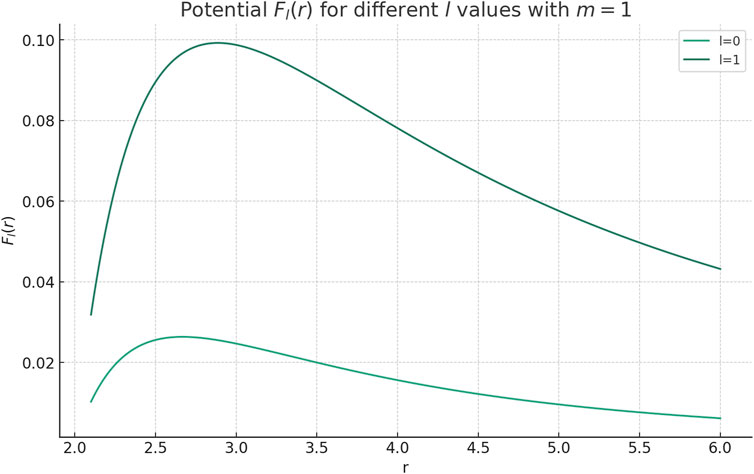
The plot displayed in Figure 2 shows the potential $F_l(r)$ as a function of $r$ for each value of $l$. Some relevant observations from the graph indicate:

$•$ The potential has a peak for each $l$, and these peaks are what we use to estimate ${\lambda }_0$.

$•$ The potential increases as $r$ increases, reaches a maximum, and then decreases again, which is a typical behavior of effective potentials and barriers.

$•$ For $l=1$, the potential reaches a higher peak than $l=0$, which aligns with the calculated ${\lambda }_0$ values where ${\lambda }_0$ for $l=1$ is greater than for $l=0$.

Figure 2

Figure 2. Potential $F_l(r)$ as a function of $r$ for $l=0$ and $l=1$.

4.1 Numerical assessments on the energy formulation

The discussion to this point has yielded an energy estimate expressed as

$E\left(t\right)\le 2E\left(0\right).$

This estimate implies that the energy of the wave function at any time $t$ does not exceed twice its initial value $E(0)$. However, this bound alone does not definitively determine how the energy evolves over time, but it does confirm that the evolution is controlled by the initial energy value. Certainly, this expression leaves open questions regarding potential energy dissipation, conservation, or other complex dynamics that could be exhibited. Hence, we conduct a numerical assessment to gain further details about whether the energy decreases or exhibits other patterns through time. We have carried out a simulation following numerical integration techniques using Python libraries. In the simulation, Gaussian initial data and a decaying sinusoidal initial time derivative were used:

${\psi }_0\left(r\right)=e^{-r^2},{\psi }_1\left(r\right)=\frac{\sin \left(r\right)}{1+r^2},$

both of which belong to $L^2$ in the domain of integration. The energy at $t=0$, denoted $E(0)$, was calculated based on these initial conditions. The plot provided in Figure 3 provides the results of the numerical analysis carried out, leading to a graph that depicts the energy $E(t)$ exponential decreasing evolution over time. This result aligns with the classical form of solutions considered to model QNMs and given by the temporal evolution $e^{-i\omega t}$, and we shall recall that our initial data were selected to belong to $L^2$.

Figure 3

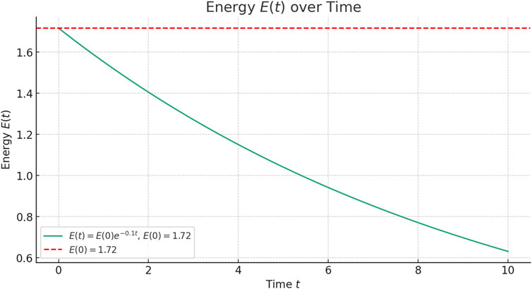
Figure 3. The energy $E(t)$ decays over time from its initial value $E(0)$. The horizontal dashed line represents $E(0)$, showing that the initial energy is constant at its initial value, while $E(t)$ decays exponentially from this initial value.

5 Conclusion

This study provided an analysis of the behavior of scalar fields in Schwarzschild spacetime using the tortoise coordinate transformation and spherical harmonics decomposition. From the numerical assessments, we established the behavior of scalar fields considering the tortoise coordinate in Figure 1 for the simplified version of the wave in (Equation 3). In addition, we have obtained estimates for the energy under the $L^2$ norm and for the evolution of the waves in the $L^{\infty }$ norm. Interestingly, we showed that a decreasing exponential bound applies for the energy evolution provided that the initial data belong to $L^2-$space. We postulate that such an evolving bound applies for any other $L^2$ initial distribution beyond the ones considered in Section 4.1. Another interesting question to explore further is how $L^2$ perturbations in the initial conditions, which introduce Kerr solutions as a second-order effect in the linearized equations, affect this obtained exponential decay. Certainly, this is a relevant issue that requires additional theoretical and numerical assessments. We will proceed with this in our future work.

Data availability statement

The original contributions presented in the study are included in the article/supplementary material, further inquiries can be directed to the corresponding author.

Author contributions

JD: conceptualization, investigation, data curation, formal analysis, funding acquisition, methodology, project administration, resources, software, supervision, validation, visualization, writing–original draft, writing–review and editing.

Funding

The author(s) declare that no financial support was received for the research, authorship, and/or publication of this article.

Conflict of interest

The author declares that the research was conducted in the absence of any commercial or financial relationships that could be construed as a potential conflict of interest.

Publisher’s note

All claims expressed in this article are solely those of the authors and do not necessarily represent those of their affiliated organizations, or those of the publisher, the editors and the reviewers. Any product that may be evaluated in this article, or claim that may be made by its manufacturer, is not guaranteed or endorsed by the publisher.

References

Balart, L., Panotopoulos, G., and Rincón, Á. (2023). Regular charged black holes, energy conditions, and quasinormal modes. Fortschr. Phys. 71, 2300075. doi:10.1002/prop.202300075

CrossRef Full Text | Google Scholar

Berti, E., Cardoso, V., and Starinets, A. O. (2009). Quasinormal modes of black holes and black branes. Class. Quantum Gravity 26, 163001. doi:10.1088/0264-9381/26/16/163001

CrossRef Full Text | Google Scholar

De Luca, V., Franciolini, G., Pani, P., and Riotto, A. (2020). The evolution of primordial black holes and their final observable spins. J. Cosmol. Astropart. Phys. 2020 (April), 052. doi:10.1088/1475-7516/2020/04/052

CrossRef Full Text | Google Scholar

Futterman, J. A. H., Handler, F. A., and Matzner, R. A. (1988). Scattering from black holes. Cambridge: Cambridge University Press.

Google Scholar

Keir, J. (2020). Wave propagation on microstate geometries. Ann. Henri Poincaré 21, 705–760. doi:10.1007/s00023-019-00874-4

CrossRef Full Text | Google Scholar

Kokkotas, K. D., and Schmidt, B. G. (1999). Quasi-normal modes of stars and black holes. Living Rev. Relativ. 2, 2. doi:10.12942/lrr-1999-2

PubMed Abstract | CrossRef Full Text | Google Scholar

Mamani, L. A. H., Masa, A. D. D., Sanches, L. T., and Zanchin, V. T. (2022). Revisiting the quasinormal modes of the Schwarzschild black hole: numerical analysis. Eur. Phys. J. C 82, 897. doi:10.1140/epjc/s10052-022-10865-1

CrossRef Full Text | Google Scholar

Martínez-Merino, A., and Sabido, M. (2022). On superstatistics and black hole quasinormal modes. Phys. Lett. B 829, 137085. doi:10.1016/j.physletb.2022.137085

CrossRef Full Text | Google Scholar

Nollert, H.-P. (1999). Quasinormal modes: the characteristic `sound' of black holes and neutron stars. Class. Quantum Gravity 16 (R159), R159–R216. doi:10.1088/0264-9381/16/12/201

CrossRef Full Text | Google Scholar

Övgün, A., Sakallı, İ., and Saavedra, J. (2018). Quasinormal modes of a Schwarzschild black hole immersed in an electromagnetic universe. Chin. Phys. C 42 (10), 105102. doi:10.1088/1674-1137/42/10/105102

CrossRef Full Text | Google Scholar

Price, R. H. (1972). Nonspherical perturbations of relativistic gravitational collapse I scalar and gravitational perturbations. Phys.Rev. D. 5, 2419–2438. doi:10.1103/physrevd.5.2419

CrossRef Full Text | Google Scholar

Regge, T., and Wheeler, J. A. (1957). Stability of a Schwarzschild singularity. Phys. Rev. 108 (4), 1063–1069. doi:10.1103/physrev.108.1063

CrossRef Full Text | Google Scholar

Rendall, A. D. (2008). Partial differential equations in general relativity. Oxford, United Kingdom: Oxford Mathematics.

Google Scholar

Sakallı, İ., and Kanzi, S. (2022). Topical Review: greybody factors and quasinormal modes for black holes in various theories - fingerprints of invisibles. Turkish J. Phys. 46 (2), 51–103. doi:10.55730/1300-0101.2691

CrossRef Full Text | Google Scholar

Sathyaprakash, B. S., and Schutz, B. F. (2009). Physics, astrophysics and cosmology with gravitational waves. Living Rev. Relativ. 12, 2. doi:10.12942/lrr-2009-2

PubMed Abstract | CrossRef Full Text | Google Scholar

Tao, T. (2006). “Nonlinear dispersive equations: local and global analysis,” in CBMS regional conference series in mathematics, 106. Providence, RI: American Mathematical Society. Provides a detailed discussion on Strichartz estimates for wave equations.

Google Scholar

Taylor, M. E. (1996). Partial differential equations: basic theory. New York: Springer.

Google Scholar

Trefethen, L. N., and Embree, M. (2005). Spectra and pseudospectra: the behavior of nonnormal matrices and operators. Princeton, NJ: Princeton University Press.

Google Scholar

Virtanen, P., Gommers, R., Oliphant, T. E., Haberland, M., Reddy, T., Cournapeau, D., et al. (2020). SciPy 1.0: fundamental algorithms for scientific computing in Python. Nat. Methods 17, 261–272. doi:10.1038/s41592-019-0686-2

PubMed Abstract | CrossRef Full Text | Google Scholar

Wald, R. M. (1984). General relativity. Chicago: University of Chicago Press.

Google Scholar

Zhao, Y., Sun, B., Mai, Z. F., and Cao, Z. (2022). Quasi normal modes of black holes and detection in ringdown process. Lausanne, Switzerland: Frontiers.

Google Scholar

Zimmerman, A., Yang, H., Mark, Z., Chen, Y., and Lehner, L. (2015). “Quasinormal modes beyond Kerr,” in Gravitational wave astrophysics. Astrophysics and space science proceedings. Editor C. Sopuerta (Cham: Springer), 40, 217–223. doi:10.1007/978-3-319-10488-1_19

CrossRef Full Text | Google Scholar