 N. A. Tsyganenko
 V. S. Semenov1
- 1Department of Physics, St. Petersburg State University, Saint Petersburg, Russia
- 2Institute of Computational Modelling of Siberian Branch of the Russian Academy of Sciences, Krasnoyarsk, Russia
- 3Applied Mechanics Cathedra, Siberian Federal University, Krasnoyarsk, Russia
Based on a new mathematical framework and large multi-year multi-mission data sets, we reconstruct electric currents and magnetic fields around the dayside magnetopause and their dependence on the incoming solar wind, IMF, and geodipole tilt. The model architecture builds on previously developed mathematical frameworks and includes two separate blocks: for the magnetosheath and for the adjacent outer magnetosphere. Accordingly, the model is developed in two stages: 1) reconstruction of a best-fit magnetopause and underlying dayside magnetosphere, based on a simple shielded configuration, and 2) derivation of the magnetosheath magnetic field, represented by a sum of toroidal and poloidal terms, each expanded into spherical harmonic series of angular coordinates and powers of normal distance from the boundary. The spacecraft database covers the period from 1995 through 2022 and is composed of data from Geotail, Cluster, Themis, and MMS, with the total number of 1-min averages about 3 M. The modeling reveals orderly patterns of the IMF draping around the magnetosphere and of the magnetopause currents, controlled by the IMF orientation, solar wind pressure, and the Earth’s dipole tilt. The obtained results are discussed in terms of the magnetosheath flux pile-up and the dayside magnetosphere erosion during periods of northward or southward IMF, respectively.
1 Introduction
The dayside magnetosheath and magnetopause play a principal role in the magnetosphere response to the interplanetary plasma flow. They serve as a main gateway where the first contact occurs between the incoming magnetized solar wind and the geomagnetic field, eventually resulting in a complex chain of magnetospheric processes. Of primary importance here is the mutual orientation of the external IMF and the internal magnetospheric field, defining the reconnection pattern at the boundary. This subject has long been at the center of many studies and extensive debates in the literature, starting from the seminal ideas of Dungey (Dungey, 1961) and followed by a multitude of works, recently summarized in reviews (Trattner et al., 2021; Fuselier et al., 2024). The reconnection geometry has been traditionally addressed in the framework of two basic concepts: the component and antiparallel merging (e.g. (Fuselier et al., 2021), and refs. therein (Qudsi et al., 2023)). A significant contribution to this area was made due to in situ measurements onboard THEMIS (Atz et al., 2022) and MMS missions (e.g. (Trattner et al., 2018; Trattner et al., 2021; Petrinec et al., 2022; Pritchard et al., 2023)). An independent insight into the problem was gained via MHD simulations, revealing in particular the importance of the Earth’s dipole tilt angle
Several studies have been made in the past to quantitatively describe the magnetic field in the domain between the bow shock and the magnetopause. Kobel and Flückiger (Kobel and Flückiger, 1994) developed an analytical theoretical model under assumption of a purely potential field and using parabolic approximation for both boundaries. In a much later work by Romashets and Vandas (Romashets and Vandas, 2019), a similar approach was employed, also based mostly on theory. An extended study of the magnetosheath properties was carried out by Zhang et al., 2019, but limited to only a statistical description of plasma and magnetic field parameters throughout the domain, without any numerical model. An in-depth data-based investigation of the IMF-controlled magnetic draping patterns in the magnetosheath was recently performed by Michotte de Welle (Michotte de Welle et al., 2022); however, that study used a direct data-driven approach, without an explicit external input.
This paper presents first results of an effort to implemenent the empirical approach to the problem, based on a formal mathematical framework and a large set of archived space magnetometer and plasma data, collected by several satellite missions over 25 + years of in situ observations. The basic goal of our work is to extend the data-constrained modeling of the magnetosphere, recently reviewed in (Tsyganenko et al., 2021), beyond the dayside magnetopause. An initial step in that direction was described in our previous paper (Tsyganenko et al., 2023) (henceforth TSE23), in which an empirical magnetosheath magnetic field model was developed. In that study, no magnetopause per se was included, and the field inside the magnetospheric boundary was tacitly implied as a smooth inward extrapolation of that in the magnetosheath, such that no Chapman-Ferraro current was included by construction. The present work is based on the same data; a new element is an explicitly defined data-derived magnetopause and an outer magnetosphere module, which makes it possible to study the IMF effects on the magnetopause current patterns.
Figure 1 illustrates the problem geometry with two field line configurations, corresponding to parallel and perpendicular IMF orientations. The plots were obtained using a simplified theoretical model with perfectly shielded vacuum fields on both sides of the magnetopause. In this work we develop a more realistic approach, including a general representation of the magnetosheath magnetic field by toroidal and poloidal components, unconstrained by the current-free assumption and based on a large pool of data.
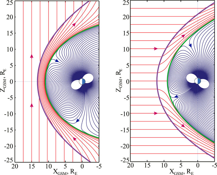
Figure 1. Illustrating the problem geometry with two IMF draping plots: for 90
The paper is organized as follows: Section 2 describes the data set, Section 3 outlines the architecture of the model, starting from a brief overview of its construction logic and followed by a more detailed description of the modular structure. Section 4 presents results of the magnetopause current calculations, Section 5 discusses the model validation and pressure balance issues, and Section 6 summarizes the article.
2 Data
As in our previous work (TSE23), the original “grand” data base included 1-min average magnetic field and plasma data, obtained over the time period from 1995 to 2022 onboard Geotail, Cluster-1, -3, -4, Themis-A, -B, -C, -D, -E, and MMS-1 missions. The data were restricted to the region sunward from
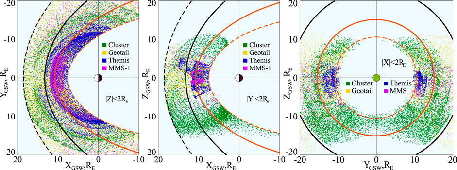
Figure 2. Spatial distribution of data records in the preliminary subset. Data of four missions are shown by different colors, as indicated in the inset legend. Only every 50th data points out of the total of 11,120,813 are plotted, limited to planar 4
At the next step, a more accurate selection of magnetosheath and magnetosphere data was performed by means of a procedure similar to that used in TSE23, employing an efficient method first proposed in (Jelínek et al., 2012). Namely, based on the measured magnetic field intensities
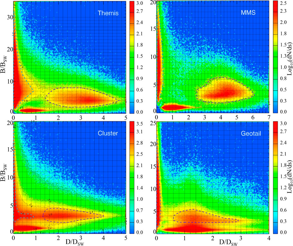
Figure 3. Four
Inevitably, the adopted selection procedure is somewhat ambiguous and subjective, which is especially evident in the cases of Geotail and Cluster, where the magnetosheath data areas continuously merge with those for the solar wind and magnetosphere, as already discussed in greater detail in TSE23 (Section 4).
In order to further reduce the uncertainties and improve the data discrimination, a second filtering procedure was applied to the data subsets obtained at the first step, based on an independent pair of region identification variables: the plasma bulk speed
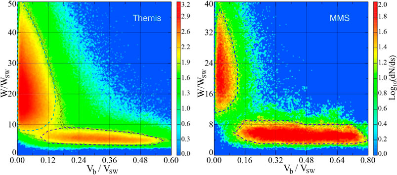
Figure 4.
Unlike Themis and MMS, the Geotail and Cluster data were not subject to the second
Table 1 displays basic statistical information about the final data set, obtained as a result of the above selection. The table’s format is similar to that of Table 1 in TSE23, but the numbers are different: first, because the present study concentrates only on the dayside magnetosheath, such that all nightside data with
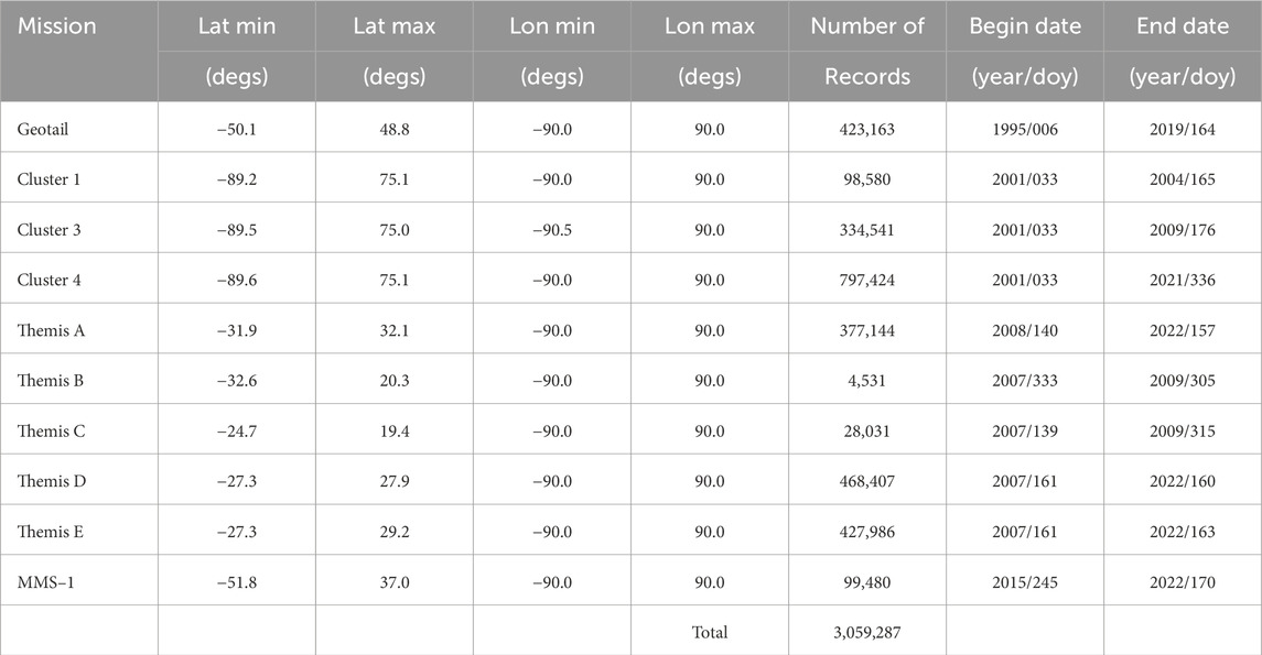
Table 1. Magnetosheath/magnetosphere data set: contributing missions, GSW latitude/longitude range, numbers of records, timespans.
Similar to what was done in TSE23, the entire fitting data pool was split into independent training (T) and validation (V) subsets. The splitting method was to divide the data records on the basis of their observation times, such that data belonging to consecutive 30-day intervals were alternately placed into the T or V subset. Because of much shorter autocorrelation times of principal interplanetary drivers (e.g. (Marquette et al., 2018)), such a method guarantees that data in the T and V subsets are sufficiently independent and, at the same time, not affected by long-term solar cycle trends. As a result of all the filtering/selection procedures, two separate T and V subsets were created containing 1,515,097 and 1,544,190 records, respectively. In the training subset, the corresponding shares of magnetosheath and magnetospheric data are, respectively, 551,231 and 963,866 records, while in the validation subset they are 557,117 and 987,073.
Finally, to avoid situations with extreme solar wind conditions, all data records with principal interplanetary parameters outside the 5%
3 Model architecture
3.1 Basic steps
The main problem with creating a joint model of the magnetosheath-magnetosphere interface region lies in drastically different magnetic geometries and field intensities on the opposite sides of the magnetopause, as well as in different timescales associated with these regions. In terms of the model architecture, this prompts to represent the magnetic field with a composite structure consisting of two separate modules and, accordingly, split the model construction into two separate tasks.
At the first step, a model of the outer dayside magnetosphere is constructed, including the derivation of best-fit magnetopause parameters and their dependence on the solar wind and IMF input. In terms of data, our focus on the dayside magnetopause suggests to assemble the modeling set in such a way that only the outermost data are selected, based on the diagrams in Figures 3, 4. Fitting the magnetospheric module to the data allows to derive such basic parameters as the magnetic field magnitude, the magnetopause standoff distance, the curvature of the boundary and its tailward flaring rate, as well as response of all the above quantities to varying solar wind and IMF conditions.
At the next step, the magnetosheath part of the model is derived, similar in its structure to that described in TSE23. More specifically, the magnetic field is represented with a sum of toroidal and poloidal parts, whose generating functions are expanded into Taylor series of the normal distance
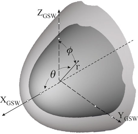
Figure 5. Coordinates used in the model formulation. Cartesian: correspond to GSW system with X-axis antiparallel to solar wind flow. Spherical: radial distance
3.2 Magnetospheric module
A principal element of the magnetospheric module is its boundary, represented here with a simple axisymmetric analytical surface first proposed in (Shue et al., 1997):
where
In principle, the magnetic field inside the magnetopause can be represented by a full-scale model, including all principal intra-magnetospheric sources such as the Earth’s dipole, magnetopause, tail, field-aligned, and ring currents ((Tsyganenko et al., 2021) or (Tsyganenko, 2013) and refs. therein). This study, however, is focused on a relatively narrow region around the magnetosheath-magnetosphere interface, which suggests to use a simpler single module like that shown in Figure 1, featuring all basic properties of the dayside field near the magnetopause:
Here the total magnetospheric field is a sum of the dipole field
where five unknown parameters
To further refine the internal field response to changing interplanetary conditions, the shielded dipole field Eq. 2 is allowed to change as a whole by the variable factor
parameterized by IMF
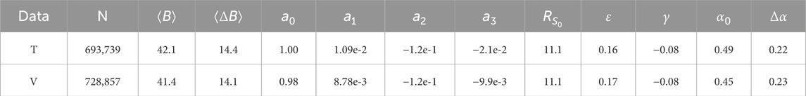
Table 2. Magnetospheric dataset and module parameters, derived by fitting to the T and V data (see Eq. 3 and text for notations). Difference between the T- and V-based values gives a rough measure of a parameter stability and error.
In total, the magnetospheric module has 9 free parameters to be found from data: four coefficients entering in Eq. 4 and five nonlinear parameters in Eq. 3. The fitting was performed using a Nelder-Mead simplex search in 5D parametric space, at each step of which the coefficients were found by a standard SVD algorithm.
In regard to all the above described formalism, a subtle issue should be highlighted: while the magnetospheric Eq. 2 is fitted to only the magnetospheric data (selected in advance by means of the diagrams in Figures 3, 4), it extends throughout the entire space as a smooth curl-free magnetic field and, hence, does not reproduce the required discontinuity of its tangential component at the magnetopause. A natural way to incorporate the magnetopause is to use the coordinate
as an independent indicator of a data point
Table 2 presents basic characteristics of both T and V magnetospheric data subsets: record numbers
3.3 Magnetosheath module
The magnetosheath magnetic field is represented by a separate mathematical framework, first described in TSE23. It is based on a sum of toroidal and poloidal components, whose generating functions are expanded into triple sums with Taylor series in powers of the normal coordinate
and
where the summation limits in Eq. 6 are as follows:
The magnetosheath module also includes the same five magnetopause parameters
The above described magnetosheath module was fitted to the training (T) and validation (V) subsets, containing, respectively, 351,069 and 355,372 data records. The corresponding r.m.s. field magnitudes were, naturally, significantly lower than those for the magnetosphere:
4 Results
4.1 Equatorial field
Figure 6 shows three dayside equatorial distributions of the magnetic field magnitude over the modeling region, corresponding to IMF
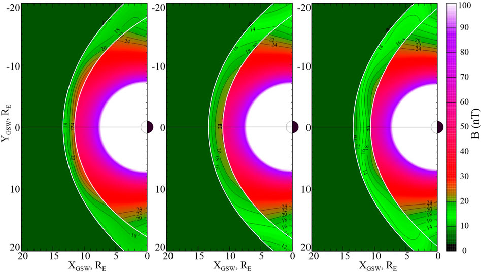
Figure 6. Equatorial plots of magnetic field magnitude for IMF B = 5 nT, IMF cone angle 90
Overall, the magnetosheath field magnitude steadily decreases with growing clock angle, reflecting the progressive decrease of the magnetic flux pile-up and increase of the dayside field erosion. In the case of purely southward IMF, two nearly symmetric and rather shallow field compression areas are formed near the magnetopause, centered at
The next Figure 7 shows in a similar format three equatorial field distributions for more commonly observed IMF orientations, corresponding to Parker spirals with a nonzero radial component:
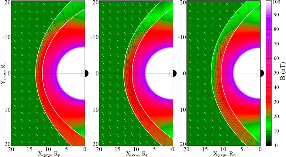
Figure 7. Distributions similar to those in Figures 6, 10, but for three spiral-type IMF orientations with
4.2 Electric currents on the magnetopause
Figure 8 shows front views of the electric current distribution on the dayside magnetopause for four values of the IMF clock angle
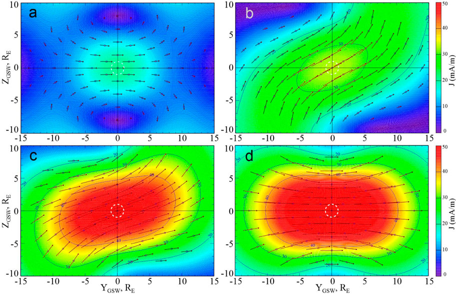
Figure 8. Color-coded electric current surface density (in mA/m) at the dayside magnetopause as viewed from the Sun, for four values of the IMF clock angle:
The next Figure 9 displays the currents in the same format and for the same IMF orientations, but for the maximum value of the dipole tilt
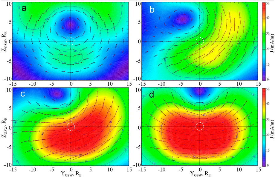
Figure 9. Same as in Figure 8, but for the maximum geodipole tilt
Also note that the deformation is not as strong in the panel (c), corresponding to the same IMF
5 Discussion: validation and pressure balance issues
As already mentioned (Section 4.1; Figures 6, 10) the modeling calculations were tested by reconstructing and comparing magnetic field configurations, based on two independent subsets of data, nearly equal in size. Another commonly used testing method is to generate a model from the training subset and compare its output with the validation data by creating scatterplots of the model field components against their observed values.

Figure 10. Same as in Figure 6 but based on the validation data subset.
Figure 11 shows a result of such a comparison; in the upper three panels, the magnetosheath model field components are plotted against the corresponding data from the training subset, while in the bottom row the model output, calculated using the training parameters, is compared with the validation data. The comparisons reveal a noteworthy difference between the plots for
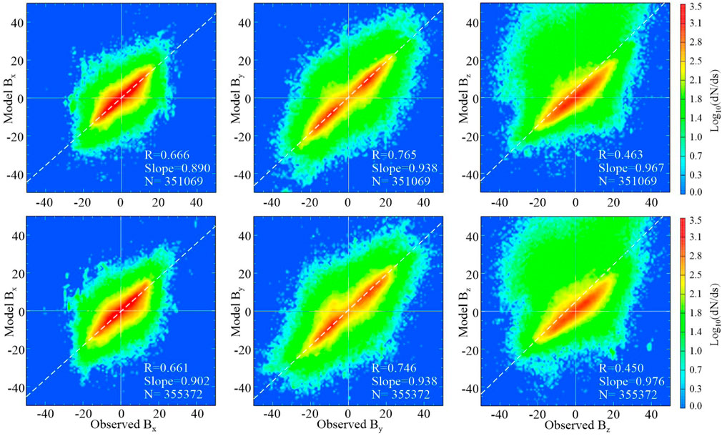
Figure 11. Scatterplots of the magnetosheath module field components against observations. Panels in the upper and lower rows correspond to the training and validation subsets, respectively. Data point numbers, Pearson correlation coefficients, and best-fit slopes are indicated in legends on each panel.
The next Figure 12 shows similar scatter plots for the magnetospheric module. Here all correlation coefficients are significantly higher, reflecting more ordered field structure and much lower noise level in the data. At the same time, all the slopes for both T and V subsets significantly exceed unity, which is obviously a result of a somewhat simplified module architecture, in which such important field sources as the ring, tail, and field-aligned currents are missing. Another possible cause is the already noted partial “diffusion” of the magnetosheath data into the magnetospheric subset. In the right panels, an overwhelming majority of data points lie in the first quadrant, due to the largely northward outer magnetospheric field.
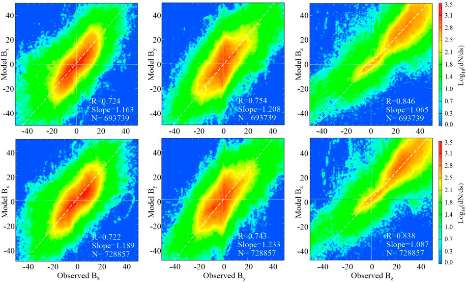
Figure 12. Same as Figure 11 but for the magnetospheric module.
Another independent test of the model’s consistency deals with the issue of net force balance between the solar wind and the magnetosphere. In particular, according to theory (Spreiter et al., 1966; Petrinec and Russell, 1997), the total pressure along the Sun-Earth line should remain constant. Left and right panels in Figure 13 display the profiles of the model magnetic field variation along the Sun-Earth line, derived from the training and validation subsets, respectively. In both cases, the IMF total magnitude equals 8.0 nT and the cone angle is 120
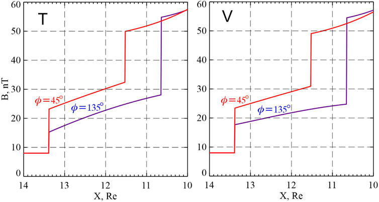
Figure 13. Variation of the total magnetic field B along the Sun-Earth line for a typical spiral-type IMF orientation, with northward IMF
The field magnitudes jump from 8 to
The first thing that draws attention in the plots is that, in both T and V variants, the plots for negative and positive IMF
As regards the overall pressure balance, in both T and V cases the subsolar field magnitudes just inside the magnetopause are in the range 50–55 nT, corresponding to the magnetic pressures
6 Summary and outlook
In this paper we presented first results of an empirical data-based modeling of the magnetic field and electric current structure at the interface between the dayside magnetosheath and the adjacent outer magnetosphere. Mathematically, the model is constructed as a composite framework consisting of two independent modules: 1) a magnetospheric module reproduced by the field of a dipole with variable strength and tilt, fully shielded within a magnetopause with variable size and shape, and 2) a magnetosheath module, based on flexible toro/poloidal expansions in a coordinate system, specially suited for the magnetopause and bow shock geometry. The experimental database includes multi-year sets of 1-min average magnetic field and plasma data of Themis, Geotail, Cluster, MMS, and OMNI source of interplanetary data. Based on a method by Jelinek et al. (Jelínek et al., 2012), the data are selected into magnetospheric and magnetosheath subsets, occupying distinctly different regions in the 2D space of normalized plasma density and magnetic field. Fitting the magnetospheric module to the data made it possible to derive not only the magnetic field, but also model magnetopause parameters, such as the standoff distance and the curvature/flaring rate of the boundary, as well as their dependence on the solar wind ram pressure and IMF
This work should be viewed as only the first step in the empirical modeling of the IMF effects on the dayside magnetosphere boundary. Our procedure of data selection and region identification is still far from being perfect, which results in a certain degree of data intermixing between different regions. The employed method based on the diagrams needs to be upgraded by taking into account as much as possible in situ telltale signatures, such as fluctuation levels of the field and plasma parameters. Another improvement area is to refine the outer magnetosphere model by including basic extraterrestrial field sources parameterized by ground-based activity indices, in order to take into account the magnetic flux redistribution between the dayside and tail lobes, which may strongly affect the position of polar cusps on the dayside. One more way to further advance the modeling is to generalize the magnetopause shape by modifying the
Data availability statement
Publicly available datasets were analyzed in this study. This data can be found here: https://cdaweb.gsfc.nasa.gov/cdaweb/sp_phys/https://omniweb.gsfc.nasa.gov/form/omni_min.html.
Author contributions
NT: Conceptualization, Data curation, Formal Analysis, Investigation, Methodology, Resources, Software, Validation, Visualization, Writing–original draft, Writing–review and editing. VS: Conceptualization, Formal Analysis, Funding acquisition, Project administration, Supervision, Writing–review and editing. NE: Conceptualization, Formal Analysis, Writing–review and editing. NG: Data curation, Writing–review and editing.
Funding
The author(s) declare that financial support was received for the research, authorship, and/or publication of this article. The authors acknowledge financial support from the Russian Science Foundation grant No. 23-47-00084 “Magnetic Reconnection in Space and Laboratory Plasmas: Computer Simulations and Empirical Modeling.”
Acknowledgments
We acknowledge the teams and PIs of all experiments whose data contributed to this study. In particular, Geotail Fluxgate Magnetometer Instrument (MGF) data were provided by the PIs, S. Kokubun (STEL), and T. Nagai (Tokyo Institute of Technology, Japan). The Geotail Comprehensive Plasma Instrument (CPI) data were obtained from NASA/GSFC NSSDC CDAWEB website (originally provided by the instrument PIs: L. A. Frank, W. Paterson, and K. Ackerson). The Cluster and MMS magnetometer/ephemeris data were obtained from the NSSDC CDAWEB online facility, originally made available by the PIs: A. Balogh and M. Tatrallyay (Cluster data), J. Burch, C. Russell, and W. Magnus (MMS data), V. Angelopoulos, K. -H. Glassmeier, U. Auster, and W.Baumjohann are acknowledged for the use of THEMIS FGM data. The Cluster and THEMIS plasma data originated from the measurements by Fast Plasma Instrument (FPI, PIs: J. Burch, C.Pollock, and B.Giles) and Electrostatic Analyzers (ESA, PIs: V. Angelopoulos, C. W. Carlson and J. McFadden), respectively; both data were provided via the NSSDC CDAWEB web interface. High-resolution OMNI interplanetary data were obtained from the SPDF OMNIWEB interface (R. McGuire, N. Papitashvili).
Conflict of interest
The authors declare that the research was conducted in the absence of any commercial or financial relationships that could be construed as a potential conflict of interest.
Publisher’s note
All claims expressed in this article are solely those of the authors and do not necessarily represent those of their affiliated organizations, or those of the publisher, the editors and the reviewers. Any product that may be evaluated in this article, or claim that may be made by its manufacturer, is not guaranteed or endorsed by the publisher.
References
Atz, E. A., Walsh, B. M., Broll, J. M., and Zou, Y. (2022). The spatial extent of magnetopause magnetic reconnection from in situ THEMIS measurements. J. Geophys. Res. Space Phys. 127, e2022JA030894. doi:10.1029/2022JA030894
Aubry, M. P., Kivelson, M. G., and Russell, C. T. (1971). Motion and structure of the magentopause. J. Geophys. Res. 77, 1673–1696. doi:10.1029/ja076i007p01673
Dungey, J. W. (1961). Interplanetary magnetic field and the auroral zones. Phys. Rev. Lett. 6, 47–48. doi:10.1103/PhysRevLett.6.47
Dušik, S., Granko, G., Šafránková, J., Němeček, Z., and Jelínek, K. (2010). IMF cone angle control of the magnetopause location: statistical study. Geophys. Res. Lett. 37 (19). Art. No. L19103. doi:10.1029/2010GL044965
Eggington, J. W. B., Eastwood, J. P., Mejnertsen, L., Desai, R. T., and Chittenden, J. P. (2020). Dipole tilt effect on magnetopause reconnection and the steady-state magnetosphere-ionosphere system: global MHD simulations. J. Geophys. Res. Space Phys. 125, e2019JA027510. doi:10.1029/2019JA027510
Fuselier, S. A., Petrinec, S. M., Reiff, P. H., Birn, J., Baker, D. N., Cohen, I. J., et al. (2024). Global-scale processes and effects of magnetic reconnection on the geospace environment. Space Sci. Rev. 220, 34. doi:10.1007/s11214-024-01067-0
Fuselier, S. A., Webster, J. M., Trattner, K. J., Petrinec, S. M., Genestreti, K. J., Pritchard, K. R., et al. (2021). Reconnection x-line orientations at the Earth’s magnetopause. J. Geophys. Res. Space Phys. 126, e2021JA029789. doi:10.1029/2021JA029789
Jelínek, K., Němeček, Z., and Šafránková, J. (2012). A new approach to magnetopause and bow shock modeling based on automated region identification. J. Geophys. Res. Space Phys. 117, A05208. doi:10.1029/2011ja017252
Kobel, E., and Flückiger, E. O. (1994). A model of the steady state magnetic field in the magnetosheath. J. Geophys. Res. Space Phys. 99 (A12), 23617–23622. doi:10.1029/94JA01778
Li, S. Y., Kronberg, E. A., Mouikis, C. G., Luo, H., Ge, Y. S., and Du, A. M. (2023). Prediction of proton pressure in the outer part of the inner magnetosphere using machine learning. Space weather. 21, e2022SW003387. doi:10.1029/2022SW003387
Lin, R. L., Zhang, X. X., Liu, S. Q., Wang, Y. L., and Gong, J. C. (2010). A three-dimensional asymmetric magnetopause model. J. Geophys. Res. 115 (A4), A04207. doi:10.1029/2009JA014235
Lu, J. Y., Zhou, Y., Ma, X., Wang, M., Kabin, K., and Yuan, H. Z. (2019). Earth’s bow shock: a new three-dimensional asymmetric model with dipole tilt effects. J. Geophys. Res. Space Phys. 124 (7), 5396–5407. doi:10.1029/2018JA026144
Marquette, M., Lillis, R. J., Halekas, J. S., Luhmann, J. G., Gruesbeck, J. R., and Espley, J. R. (2018). Autocorrelation study of solar wind plasma and IMF properties as measured by the MAVEN spacecraft. J. Geophys. Res. Space Phys. 123, 2493–2512. doi:10.1002/2018JA025209
Mead, G. D., and Beard, D. B. (1964). Shape of the geomagnetic field solar wind boundary. J. Geophys. Res. 69, 1169–1179. doi:10.1029/jz069i007p01169
Michotte de Welle, B., Aunai, N., Nguyen, G., Lavraud, B., Génot, V., Jeandet, A., et al. (2022). Global three-dimensional draping of magnetic field lines in Earth’s magnetosheath from in-situ spacecraft measurements. J. Geophys. Res. Space Phys. 127, e2022JA030996. doi:10.1029/2022JA030996
Petrinec, S. M., Burch, J. L., Fuselier, S. A., Trattner, K. J., Giles, B. L., and Strangeway, R. J. (2022). On the occurrence of magnetic reconnection along the terrestrial magnetopause, using Magnetospheric Multiscale (MMS) observations in proximity to the reconnection site. J. Geophys. Res. Space Phys. 127, e2021JA029669. doi:10.1029/2021JA029669
Petrinec, S. M., and Russell, C. T. (1997). Hydrodynamic and MHD equations across the bow shock and along the surfaces of planetary obstacles. Space Sci. Rev. 79, 757–791 97. doi:10.1023/A:1004938724300
Pritchard, K. R., Burch, J. L., Fuselier, S. A., Genestreti, K. J., Denton, R. E., Webster, J. M., et al. (2023). Reconnection rates at the Earth’s magnetopause and in the magnetosheath. J. Geophys. Res. Space Phys. 128, e2023JA031475. doi:10.1029/2023JA031475
Qudsi, R. A., Walsh, B. M., Broll, J., Atz, E., and Haaland, S. (2023). Statistical comparison of various dayside magnetopause reconnection X-line prediction models. J. Geophys. Res. Space Phys. 128, e2023JA031644. doi:10.1029/2023JA031644
Romashets, E. P., and Vandas, M. (2019). Analytic modeling of magnetic field in the magnetosheath and outer magnetosphere. J. Geophys. Res. Space Phys. 124, 2697–2710. doi:10.1029/2018JA026006
Samsonov, A. A., Gordeev, E., Tsyganenko, N. A., ŠafránkováNěmeček, Z., Šimunek, J., Sibeck, D. G., et al. (2016). Do we know the actual magnetopause position for typical solar wind conditions? J. Geophys. Res. Space Phys. 121, 6493–6508. doi:10.1002/2016JA022471
Shue, J.-H., Chao, J. K., Fu, H. C., Russell, C. T., Song, P., Khurana, K. K., et al. (1997). A new functional form to study the solar wind control of the magnetopause size and shape. J. Geophys. Res. Space Phys. 102 (5), 9497–9511. doi:10.1029/97JA00196
Spreiter, J. R., Summers, A. L., and Alksne, A. Y. (1966). Hydromagnetic flow around the magnetosphere, Planet. Space Sci. 14 (3), 223–250. doi:10.1016/0032-0633(66)90124-3
Trattner, K. J., Burch, J. L., Cassak, P. A., Ergun, R., Eriksson, S., Fuselier, S. A., et al. (2018). The transition between antiparallel and component magnetic reconnection at Earth’s dayside magnetopause. J. Geophys. Res. Space Phys. 123, 10,177–10,188. doi:10.1029/2018JA026081
Trattner, K. J., Petrinec, S. M., and Fuselier, S. A. (2021). The location of magnetic reconnection at Earth’s magnetopause. Space Sci. Rev. 217, 41. doi:10.1007/s11214-021-00817-8/
Tsyganenko, N. A. (1995). Modeling the Earth’s magnetospheric magnetic field confined within a realistic magnetopause. J. Geophys. Res. Space Phys. 100, 5599–5612. doi:10.1029/94ja03193
Tsyganenko, N. A. (2013). Data-based modelling of the Earth’s dynamic magnetosphere: a review. Ann. Geophys. 31 (10), 1745–1772. doi:10.5194/angeo-31-1745-2013
Tsyganenko, N. A., Andreeva, V. A., and Gordeev, E. I. (2015). Internally and externally induced deformations of the magnetospheric equatorial current as inferred from spacecraft data. Ann. Geophys. 33 (1), 1–11. doi:10.5194/angeo-33-1-2015
Tsyganenko, N. A., Andreeva, V. A., Kubyshkina, M. V., Sitnov, M. I., and Stephens, G. K. (2021). “Data-based modeling of the Earth’s magnetic field,” in Space physics and aeronomy collection volume 2: magnetospheres in the solar system, geophys. Monogr. American geophysical union. Editors R. Maggiolo, N. Andre, H. Hasegawa, and D. T. Welling First Edition (Hoboken: Wiley and Sons, Inc.), 259. doi:10.1002/9781119815624.ch39
Tsyganenko, N. A., and Fairfield, D. H. (2004). Global shape of the magnetotail current sheet as derived from Geotail and Polar data. J. Geophys. Res. Space Phys. 109, A03218. doi:10.1029/2003ja010062
Tsyganenko, N. A., Semenov, V. S., and Erkaev, N. V. (2023). Data-based modeling of the magnetosheath magnetic field. J. Geophys. Res. Space Phys. 128, e2023JA031665. doi:10.1029/2023JA031665
Tsyganenko, N. A., and Sibeck, D. G. (1994). Concerning flux erosion from the dayside magnetosphere. J. Geophys. Res. Space Phys. 99 (7), 13,425–13,436. doi:10.1029/94ja00719
Tsyganenko, N. A., and Usmanov, A. V. (1984). Effects of the dayside field-aligned currents in location and structure of polar cusps. Planet. Space Sci. 32 (1), 97–104. doi:10.1016/0032-0633(84)90045-x
Vokhmyanin, M. V., Stepanov, N. A., and Sergeev, V. A. (2019). On the evaluation of data quality in the OMNI interplanetary magnetic field database. Space weather. 17, 476–486. doi:10.1029/2018SW002113
Keywords: magnetosphere, magnetosheath, magnetopause, modeling, solar wind, IMF
Citation: Tsyganenko NA, Semenov VS, Erkaev NV and Gubaidulin NT (2024) Magnetic fields and electric currents around the dayside magnetopause as inferred from data-constrained modeling. Front. Astron. Space Sci. 11:1425165. doi: 10.3389/fspas.2024.1425165
Received: 29 April 2024; Accepted: 18 June 2024;
Published: 18 July 2024.
Edited by:
Zerefsan Kaymaz, Istanbul Technical University, TürkiyeReviewed by:
Zdenek Nemecek, Charles University, CzechiaBayane Michotte De Welle, UMR7648 Laboratoire de physique des plasmas (LPP), France
Copyright © 2024 Tsyganenko, Semenov, Erkaev and Gubaidulin. This is an open-access article distributed under the terms of the Creative Commons Attribution License (CC BY). The use, distribution or reproduction in other forums is permitted, provided the original author(s) and the copyright owner(s) are credited and that the original publication in this journal is cited, in accordance with accepted academic practice. No use, distribution or reproduction is permitted which does not comply with these terms.
*Correspondence: N. A. Tsyganenko, bi50c3lnYW5lbmtvQHNwYnUucnU=