 D. E. da Silva
 S. R. Elkington
 X. Li
X. Li M. K. Hudson2
 A. J. Boyd
 A. N. Jaynes
 M. Wiltberger
94% of researchers rate our articles as excellent or good
Learn more about the work of our research integrity team to safeguard the quality of each article we publish.
Find out more
METHODS article
Front. Astron. Space Sci., 04 July 2024
Sec. Space Physics
Volume 11 - 2024 | https://doi.org/10.3389/fspas.2024.1423545
This article is part of the Research TopicThe Loss and Acceleration Mechanisms of Energetic Electrons in the Earth’s Outer Radiation BeltView all 10 articles
The reprocessing of radiation belt electron flux measurements into phase space density (PSD) as a function of the adiabatic invariants is a widely-used method to address major questions regarding electron energization and loss in the outer radiation belt. In this reprocessing, flux measurements j (α, E) at local pitch angles α, energies E, and optionally magnetometer measurements B, are combined with a global magnetic field model to express the phase space density f (L*) in terms of the third invariant Φ ∝ 1/L* at fixed first and second invariants M and K. While the general framework of the calculation is agreed upon, implementation details vary amongst the literature, and the issue of magnetic field model dependence is rarely addressed. This work reviews the steps of the calculation with lists of commonly used implementation options. For the first time, analysis is presented to display the effect of doing the calculation with different implementation options and with different backing models (including both empirical and MHD-driven models). The results are summarized to inform evaluation of existing results and future efforts calculating and analyzing radiation belt electron phase space density. Three events are analyzed, and while differences are found, the primary structural interpretations of the phase space density analysis exhibit model independence.
The outer radiation belt is home to fluxes of energetic (MeV) electrons which are notable due to their presence alongside critical spacecraft assets vulnerable to negative side-effects from energetic particle impacts. The variability over time of such electron fluxes occurs over many orders of magnitude. While the fundamental periodic motion of these trapped particles is understood (Roederer and Zhang, 2016), many open questions around the processes involved in their acceleration and loss remain (Reeves et al., 2003; Green and Kivelson, 2004).
Many candidate mechanisms which could affect the radiation belt populations have been identified. Loss is generally understood to occur (a) from precipitation into the atmosphere, forced by diffusive changes to the pitch angle distribution function via wave-particle interactions and atmospheric precipitation, or (b) abrupt changes to the magnetopause location that remove particles from their trapped trajectories (Jaynes and Usanova, 2019).
Acceleration is understood to arise from two families, distinguished by the time-varying patterns in the global pitch angle distribution of trapped particle states. These two mechanisms are radial transport and local acceleration (Green and Kivelson, 2004; Reeves et al., 2013; Boyd et al., 2018). Radial transport (sometimes referred to as external acceleration or radial diffusion in the literature) is understood to occur from Ultra Low Frequency (ULF) wave-particle interactions, which move particles across L-shells faster than the particle’s drift can adjust, causing the particle energy to increase to preserve its first and second invariant in a stronger magnetic field. Local acceleration (sometimes also referred to as growing peak acceleration or internal acceleration in the literature) is driven by gyro-resonant waves (such as chorus) and accelerates particles at their existing locations around L < 6.6 (Horne et al., 2005; Thorne et al., 2013). The question of which mechanisms accelerate electrons is further complicated by the possibility that a mix of mechanisms may exist simultaneously, with recent results suggesting that internal acceleration may be dominant for some energy ranges (3–5 MeV electrons), while radial transport may be dominant for others (∼7 MeV) (Zhao et al., 2018).
The observational study of outer radiation belt electron enhancements is made difficult due to response of the directly observed flux distribution from the changing storm-time global magnetospheric magnetic field. The directly observed differential directional flux distribution (henceforth just abbreviated as flux) is typically measured in the form j (E, α; x, t), where j is the flux, E is the electron energy, α is a local pitch angle, x is the location of the spacecraft, and t is the time of measurement. Even in the absence of accelerating wave-particle interactions, a particle measured at a position and a local time with distribution coordinate (E, α) may possibly never return to that local time with the same (E, α). This is due to adiabatic changes to its Cartesian trajectory, pitch angle, and drift shell brought about from changes to the global magnetospheric magnetic field. For reasons such as these, studies tracking a measured observable such j (E0, α0; x, t), where E0 is a fixed energy and α0 is a fixed local pitch angle, are severely limited.
Instead, it has become common to combine modeling of the global magnetospheric magnetic field with observations to cast the flux in terms of adiabatic invariant coordinates. These coordinates function as an underlying measure of the trapped state, and remain constant, provided the global magnetospheric magnetic field changes slowly compared to the drift period. These adiabatic invariant coordinates, in order, are (1) M or μ, corresponding to the relativistic and non-relativistic magnetic moment respectively, (2) I or J or Kcorrespond to an integral over the bounce motion, and (3) Φ or L* corresponding an integral over the drift shell (Roederer and Zhang, 2016). The adiabatic invariants themselves, can be derived from action integrals taken over one period of the periodic motion (Schulz, 1996).
The conversion of flux to a quantity known as phase space density and recasting of the coordinates in terms of adiabatic invariants is known as phase space density analysis, which results in the model-supplement measurement f (M, K, L*) (Chen et al., 2006; Iles et al., 2006; Turner et al., 2013; Kim et al., 2023). Typically, to aid visualization, M and K are held constant, and one curve of f (L*) per inbound/outbound arm of an orbit is plotted. This curve can then be used to demonstrate changes to the (M, K) population at each L*, which may occur from additions, losses, or redistribution of a (M, K) population across L*.
The implementation details of combining a flux measurement with a global magnetic field model vary amongst the literature. Most commonly, the global magnetic field model used is an empirical model, often either Tsyganenko models TS05 and T96 (Tsyganenko, 1996; Tsyganenko and Sitnov 2005). More recently, the calculation of adiabatic invariants from output of magneto-hydrodynamic (MHD) simulations has appeared in the literature (da Silva et al., 2022). In this manuscript, we seek to answer the question as to whether the interpretation of phase space density analysis differs dramatically when the same data is reprocessed using different models. In this study, we use data from two empirical models and two MHD-driven simulations: T96 (empirical), TS05 (empirical), the Space Weather Modeling Framework (SWMF; an MHD model; Tóth et al. (2005)) and Lyon-Fedder-Mobarry (LFM; an MHD model; Lyon et al. (2004)), both at similar resolutions and coupled with the Rice Convection Model (RCM; Toffoletto et al. (2003)) for stronger ring current modeling.
The magnetic field model is not the only implementation detail which varies amongst the literature. Aside from issues of magnetic field model and the calculation of the invariants themselves, differences in the numerical methods to convert the flux measurement to phase space density at the given adiabatic invariant coordinate arise in the literature. Among these numerical differences are different approaches to fitting and interpolation, done with different degrees of agency applied to smoothing of the measurements.
To illustrate the numerical differences, we will give a motivating example. In the calculation, which will be described step-by-step later on, there is a step where the flux j (E, α) is put in terms of just j(E), and it is required to interpolate this curve at a fixed E. Methods for interpolating j(E) are as follows:
• Fitting j(E) to a power law distribution (Hartley and Denton, 2014)
• Converting j(E) to f(E) and fitting to an exponential distribution (Green and Kivelson, 2004)
• Use of a smoothing spline for the j(E) curve with both the dependent and independent variables in log space (Boyd et al., 2014; Boyd et al. 2018; Boyd et al. 2021)
In this work, we will demonstrate that the choice for this step is in some cases significant enough that changing the approach causes a result that exhibits evidence of internal acceleration to change to a result that exhibits evidence of radial diffusion.
In order to strengthen the foundation of the phase space density analysis methodology and related results in the literature, this manuscript aims to study the effect of model dependence and implementation options not related to the model used. By doing this, we aim to provide a more stable groundwork for this computational technique in relating radiation belt theory to observational evidence.
This paper consists of three sections; Data and Models, Calculation Analysis, and Model Dependence. In the Data and Models section, we describe the data and models used for this study. In the Calculation Analysis section we review each step of the calculation, along with the different implementation options known to exist. Discussion is made between the different implementation options with commentary as to which are important and which are minor, and plots are presented showing the differences in doing the calculation each way. This section does not intend to cover every numerical approach which may be used (such would be impossible to cover within an article), but instead covers the most reasonable and widely used approaches in the community. In the Model Dependence section, we use a set of nominal implementation options for the algorithm and apply them with different magnetic field models, studying the differences in the results for three different classes of radiation belt enhancements. These classes are taken from the previous work of (Boyd et al., 2018), and correspond to (a) Growing Peak Events, (b) Flat Gradient Events, and (c) Positive Gradient Events.
The only required measurement to perform a phase space density analysis is that of a flux distribution over time j (E, α; x, t) which, if not directly available in a mission dataset, can be computed from j (v; x, t) or j (p; x, t) where v is a velocity and p is a momentum and a value of B at the spacecraft location. Strictly speaking, a measurement of B is not required, as one can attempt to acquire B from evaluating the model at the spacecraft location, though that is less desirable.
In this study, we use data from Van Allen Probes Energetic Particle, Composition, and Thermal Plasma (ECT) suite (Spence et al., 2013). Specifically, we use the Level-3 RBSP-ECT combined pitch angle resolved electron flux data product (Boyd et al., 2021). This Level-3 dataset bins the data into 3-min time resolution and inter-calibrates the multiple ECT instruments of the (a) Helium, Oxygen, Proton, and Electron (HOPE) (Funsten et al., 2013), (b) Magnetic Electron Ion Spectrometer (MagEIS) (Blake et al., 2013), and (c) Relativistic Electron Proton Telescope (REPT) (Baker et al., 2012). While the dataset includes precomputed values for invariants I and L* using the Olson & Pfitzer Quiet-time Model for the external field (Olson and Pfitzer, 1974) and the International Geomagnetic Reference Field (IGRF; Macmillan and Maus (2005)) calculated using LANLGeoMag software (Henderson et al., 2024), we do not use those. Instead we calculate our own values using methodology described in da Silva et al. (2024) and the models to be discussed later in this section.
We also use data from the Van Allen Probes magnetometer, Electric and Magnetic Field Instrument Suite and Integrated Science (EMFISIS; Kletzing et al. (2013)). Specifically, we use the 4-s time resolution data product (C.A. Kletzing (2022)).
In a phase space density analysis, models of the magnetospheric magnetic field are used to provide a value for B (x, t) throughout the magnetosphere. Strictly speaking, it is only required to cover (a) the drift shell of the target (M, K) particle class at each L*, and (b) the highest north/south latitude reached on the bounce path of the most non-equatorial measured pitch angle at each spacecraft position. In practice, it is easiest to assume modeling capability for everywhere between the lower boundary of the model and a few RE above the spacecraft apogee (to allow for effects such as drift shell splitting).
Models which may be used include the class of empirical models, derived largely from spacecraft measurements and supporting structural physics, and the class of dynamic simulations such as those driven primarily by MHD. In this study we use two empirical models, the Tyganenko 1996 model (T96; Tsyganenko (1996)) and the Tsyganenko/Sitnov 2005 model (TS05; Tsyganenko and Sitnov (2005)). Because our invariant calculation code is designed around gridded magnetic fields, these models were evaluated on a rectilinear grid with each X, Y, and Z-axes between −10 RE and +10 RE with grid spacing of 0.15 RE. Experimentation was done with the grid resolution and it was found that using a lower grid resolution did not change the results of this work. This outer boundary of ±10 RE is safely outside the Van Allen Probes apogee of 5.8 RE. The T96 and TS05 models are driven by a combination of interplanetary magnetic field (IMF) and Dst index measurements. The TS05 model is driven by these but also by precomputed W parameters W1 − W6 that model persistence in the magnetosphere, including but not limited to ring current buildup. The IMF and W parameters used are supplied by the 5-min time resolution Qin-Denton dataset, hosted at George Mason University.
The MHD-driven models used here are the Space Weather Modeling Framework (SWMF; Tóth et al. (2005)) and Lyon-Fedder-Mobarry (LFM; Lyon et al. (2004)), both at similar resolutions and coupled with the Rice Convection Model (RCM; Toffoletto et al. (2003)) to model the ring current. The runs were done using the Community Coordinated Modeling Center (CCMC) Run-on-Request system (https://ccmc.gsfc.nasa.gov/). The 2023 version of SWMF was used, with the auroral ionosphere conductance setting and no corotation velocity applied at the inner boundary. The SWMF simulation was performed on a grid with 4,873,456 cells with 1/8 RE resolution at the inner boundary. The LTR-2_1_5 version of LFM was used, also with the auroral ionosphere conductance setting and no corotation velocity applied at the inner boundary. The LFM simulation was performed on a grid with 1,302,528 cells (106 × 96 × 128). In subsequent figures, the simulations are referred to as SWMF-RCM and LFM-RCM to emphasize all coupled components involved. When MHD-driven models are used, the simulation is driven by solar wind boundary conditions. In this work, the solar wind boundary conditions are taken from the OMNI data product, which is derived from spacecraft measurements around L1. Such spacecraft include ACE (Chiu et al., 1998) and Wind (Ogilvie et al., 1995; Ogilvie and Desch, 1997). No special settings at the CCMC were used regarding OMNI.
The seven steps of the calculation are outlined in Figure 1. When applicable, different implementation options for fulfilling each step are presented. These options were collected by reviewing key examples in the literature and consulting with members of the community. They are intended to represent the most reasonable and common approaches, rather than a fully extensive set of all possible approaches. In this section, we will walk through each individual step, discussing the different implementation options listed, with a particular eye towards how each option may effect the analysis’ effectiveness at organizing the data so as to distinguish between signatures of internal acceleration and radial transport.
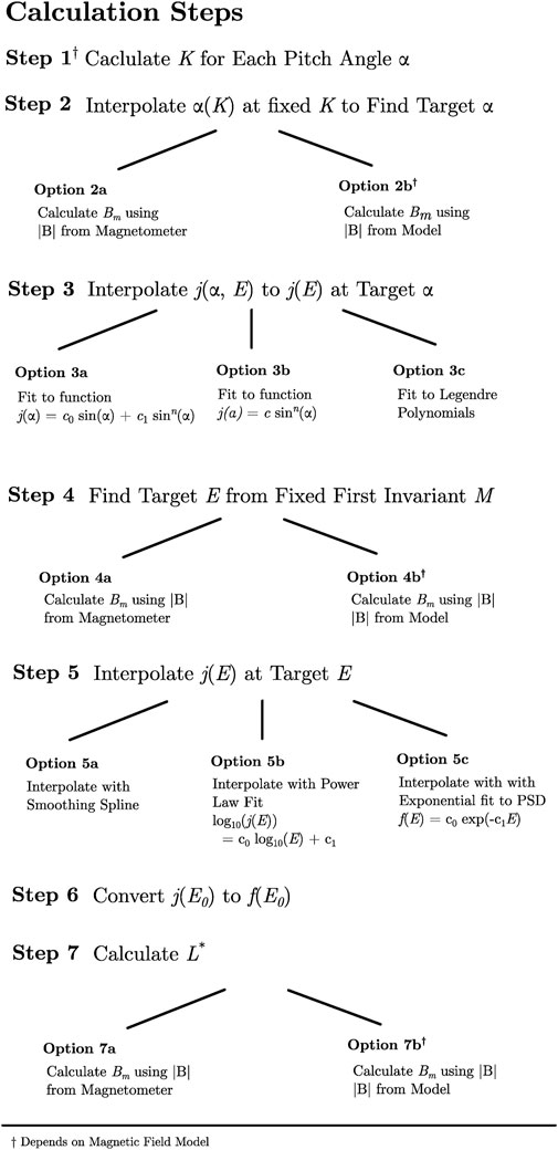
Figure 1. Steps of the phase space density calculation, per timestep, using a fixed M and K selected for the computation.
The calculation steps are presented in terms of what to do for each time step. The calculation is done for particular fixed M and K which is to be selected beforehand. In general, higher K correspond to equatorial pitch angles farther away from 90°, and higher M correspond to higher perpendicular energies at the magnetic equator.
Step 1 begins with pairing each pitch angle αi of the data with a counterpart Ki, using separate code to calculate the second invariant K using a magnetic field model. Konstantinidis and Sarris (2015) have investigated the differences in the calculated second invariants (they used I or K) between invariant calculation codes and backing magnetic field models. They found that there was generally good agreement between the codes tested for evaluation of the second invariant. The codes evaluated in that work were IRBEM (Boscher et al., 2022), SPENVIS (Heynderickx et al., 2000; Kruglanski et al., 2009), and a particle tracer.
The second step is to interpolate the curve of (Ki, αi) from the previous step to determine the calculation’s target pitch angle from the target fixed K selected. A reasonable way to interpolate α(K) is using linearly interpolation with K in log space. Experiments were performed where we interpolated α(K) using splines and it was found that differences were non-consequential.
Step 3 includes more variation in the implementation options. In this step, one interpolates the j (α, E) flux measurement at the target α found from Step 2, and produces a one-dimensional j(E) curve. This step can be done by stepping through each energy channel and fitting the pitch angle flux distribution at that energy to a functional form which is then interpolated. This is best done in combination with time averaging to mitigate the effects of noise that may result from low counting statistics.
Methods for fitting this functional form include fitting to the following functional form:
which was used early on in phase space density analysis in Green and Kivelson (2004) and stated to be designed as a method of fitting both butterfly and highly peaked distributions. Other methods include the simpler functional form (Gannon et al., 2007; Selesnick and Kanekal, 2009; Gu et al., 2011; Ni et al., 2015),
which may be easier to numerically fit (Vampola, 1998), but is capable of modeling fewer pitch angle distribution shapes. In the work of Boyd et al. (2021) a method is presented which fits log10 (j(α)) to a set of orthogonal basis functions known as the Legendre polynomials, which have the added benefit that the fitted j(α) may be guaranteed symmetric through the use of only even-term basis functions, which is desirable as a method of removing noise when j(α) truly is symmetric.
Step 5 involves finding the target E where we will interpolate along the j(E) curve. This is done by using the fixed first invariant M, which can be written as a function of E, our target α, and the magnetic field strength |B|. The equation for M written this way is (Hartley and Denton, 2014),
When α, M, and |B| are known and E is considered the independent variable, this can be solved as a quadratic equation. The real solution for E is given by,
The implementation variation for this step comes from whether to take |B| from the model or an onboard magnetometer. Strictly speaking, the |B| in Eq. 3 corresponds to the magnetic field averaged over a gyration (Chen, 1984), but it is common practice to use |B| at the spacecraft location as a simplification.
When the target E is obtained, Step 5 involves interpolating the j(E) curve at the target E. This j(E) curve is expressed from Step 3 in data as a series of points, and the most common approaches to interpolating involve fitting it to a smoother function and then evaluating that function at the target E. Methods of doing so include (a) using a smoothing spline such as with the make_smoothing_spline() function in the Python SciPy package (Virtanen et al., 2020), (b) fitting to a power law distribution (Hartley and Denton, 2014), or (c) converting to units of phase space density and fitting to an exponential distribution (Green and Kivelson, 2004). Our experiments yielded the conclusion that a smoothing spline produced the best results, both due to visual inspection, the smoothing spline’s ability to adapt to structure in j(E) without a priori assumptions about that structure, and even the ability to adapt to reverse energy spectra with higher fluxes at higher energies (Zhao et al., 2019). Experiments were done with a non-smoothing spline (specifically a cubic spline), and it was found this degraded results over the smoothing spline due to effects of instrument noise.
In Figure 2 we display a phase space density analysis with this step performed using a smoothing spline and a power law fit. For this experiment, options 2a, 3c, 4a, 5a, and 7a of Figure 1, were used and the background model was SWMF-RCM. In this example, use of the power law distribution for interpolating j(E) over a smoothing spline leads to very different conclusions regarding whether the event exhibits signatures of local acceleration (left) or radial transport (right). On the left panel, one can see a clear unimodal distribution whose peak increases in time, consistent with the local acceleration theory of (Boyd et al., 2018) energizing wave-particle acceleration occurring around L* ∼ 4.5 in this plot. While on the right, one can see the phase space density at high L* ∼ 5.5 remaining high and steady, while the phase space density at lower L* is gradually increasing consistent with radial transport acceleration (Elkington, 2006). Figure 3.
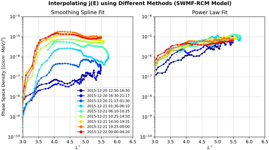
Figure 2. Two different options for satisfying Step 5 (Figure 1), which lead to very different conclusions regarding whether the event exhibits signatures of local acceleration (left) or radial transport (right). Per discussion in the text, the smoothing spline fit is the recommended option, with the power law distribution deemed a poor fit for the data observed (as illustrated in Figure 3).
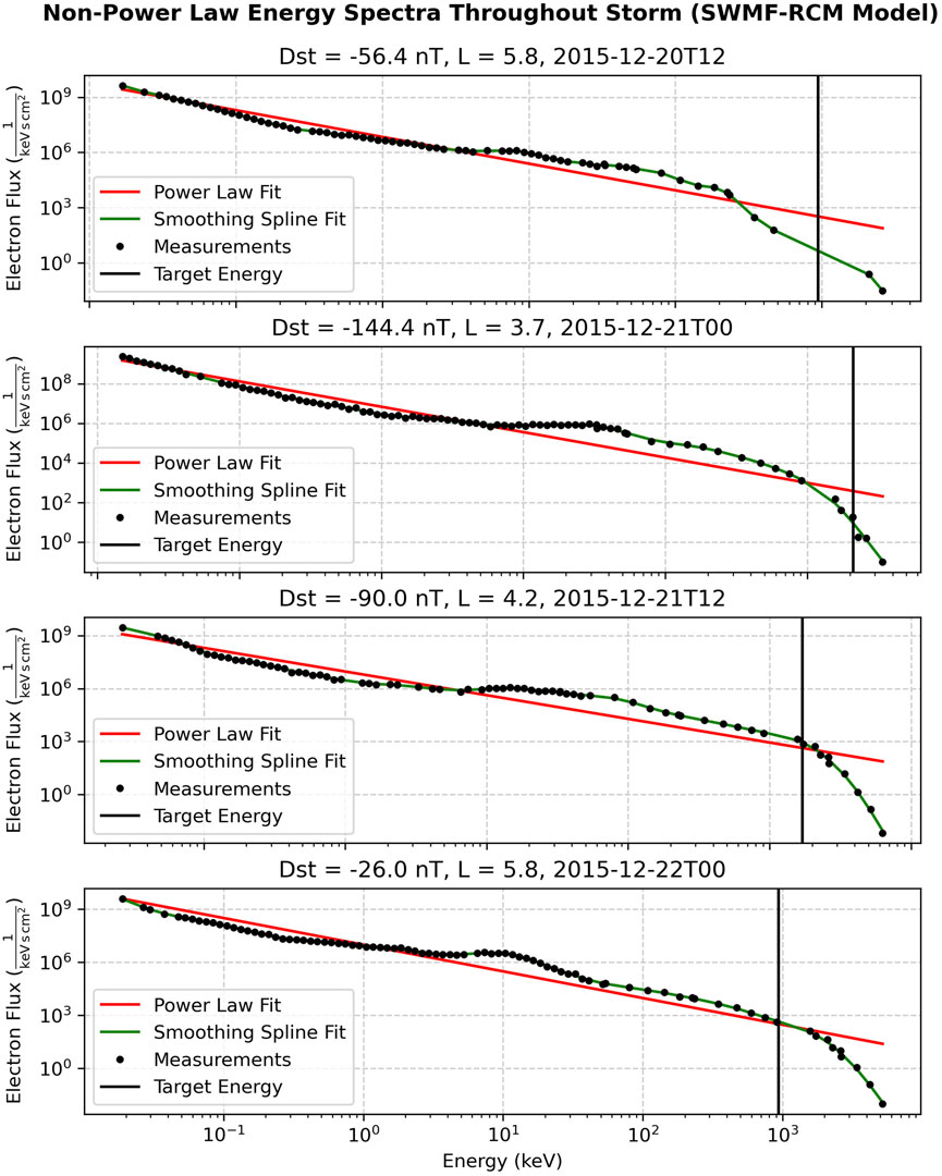
Figure 3. Further illustration depicting the issues with interpolating j(E) using a power law distribution fit. In this plot we also notice that the target energy we interpolate (vertical black light) changes throughout a storm in response, leading to interpolation between different energy channels and possibly even between different instruments.
The deeper issues with the power law fit of the j(E) curve is displayed in Figure 3, showing multiple fits over the course of the same event shown in Figure 2 (and later in Section 4.1). While the power law distribution may be an appropriate fit for certain subset energy ranges of the j(E) curve, it is a poor fit for the full energy range, and yields over or under estimates in almost every panel shown. In this plot the vertical black bar, placed at the target energy E, increases during the main phase of the storm, and decreases during the recovery time in accordance to changing variables in Eq. 4. We notice that at high energies, particularly above 1 MeV, noise is visible in the j(E) data, which can be connected to lower counting statistics within the instrument. Variations of the power law fit, such as fitting only energies above 50 keV, were evaluated and yielded similarly poor results. We conclude that the smoothing spline represents the strongest approach to satisfying this step.
In Step 6, when the j (E0) flux value is found, this value is converted to phase space density using the basic equation,
where p is the relativistic momentum.
Now that a phase space density f has been computed for this time step, the final remaining Step 7 involves assigning a value of L* for this point. Similar to the calculation of K in Step 2, this can be done with different codes and algorithms for computing the invariants. The implementation option we consider here is similar to Step 2, which is whether the mirror point strength Bm used in the calculation is derived using the |B| from the magnetometer or |B| from the model.
In Figure 4 we consider the effect of using |B| from the magnetometer or |B| from the model jointly for the entire calculation. This choice comes into play for options 2a/2b, 4a/4b, and 7a/7b in Figure 1. To simplify the analysis, an experiment was done where |B| was always used from the magnetometer (2a, 4a, 7a) and always from the model (2b, 4b, 7b). It was found that the effect of this difference is very minor, and doing it either way leads to a similar interpretation of a growing peak event. Some minor differences in the lines appear, most notably in the line labeled 2015-12-20 21:17-01:30. This line corresponds to around the Dst minimum of the storm, where it can be expected that agreement in |B| between the model and the magnetometer is most difficult (da Silva et al., 2024). Overall, the conclusion from this study is that the difference in using |B| from either magnetometer or model is of low impact on the final result, provided one avoids poor models.

Figure 4. This plot shows the only very minor differences that were found when a phase space density analysis was done two ways: (left) using |B| from magnetometer observation, and (right) using |B| from the model. Per the implementation option numbering of Figure 1, the left panel depicts options 2a/4b/7a, and the right panel depicts options 2b/4b/7b in Figure 1.
We note, still, that differences in L* between models do exist, and warrant consideration. This is investigated in more detail in the next section.
The three events presented here are used as canonical examples of three corresponding classes of radiation belt enhancement. These are (a) growing peak events, (b) flat gradient events and (c) positive gradient events. Growing peak events are de facto examples of internal acceleration, with the other two events inviting alternate interpretation. Growing peak events are defined as those which clearly resolve a growing peak within the Van Allen Probes apogee of 5.8 RE, while flat gradient events exhibit either flat or slightly negative gradients (∂f/∂L* ≈0 or ∂f/∂L* <0) at the Van Allen Probes apogee. Positive gradient events are similar, but have positive monotonic gradients (∂f/∂L* >0) at the Van Allen Probes apogee.
In Boyd et al. (2018), 80 outer radiation belt events between October 2012 to April 2017 were analyzed and sorted into these three categories. A key result of that study was that 87% of those events exhibited growing peaks, which suggests that internal acceleration mechanisms are common, but perhaps not exclusively the story of what causes energetic electron enhancements in the radiation belts.
The influence of the magnetic field model enters the calculation in the final calculation of L* (Step 7), but also more subtly when α is paired with K to determine the pitch angle which corresponds to the fixed K being analyzed (Step 1). In this section, we investigate three events previously written about in Boyd et al. (2018), reproducing previous results in the literature using multiple background magnetic field models.
In Boyd et al. (2018) the TS05 model was used. The plots displayed in this section utilize the implementation option prescription 2a/3c/4a/5a/7a per Figure 1, which fits the pitch angle flux distribution to Legendre polynomials, uses a smoothing spline to interpolate j(E), and favors using the magnetometer |B| over the model |B| in every instance. Values of M = 794 MeV/G and
In Figure 5, we process the 20 December 2015 growing peak event using the TS05 (Empirical), T96 (Empirical), SWMF-RCM (MHD), and LFM-RCM (MHD) models. The solar wind
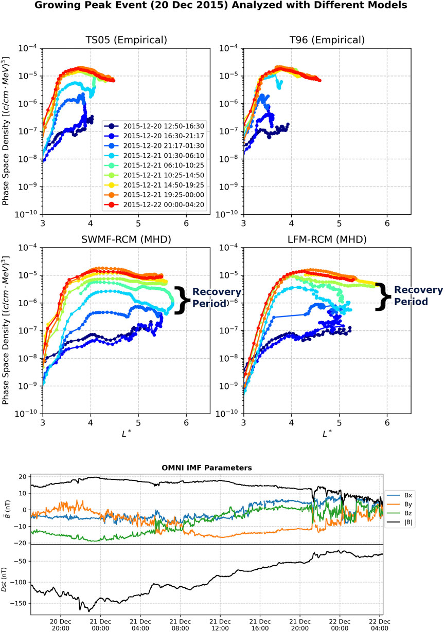
Figure 5. A growing peak (internal acceleration) event starting around 20 December, 2015. The phase space density analysis here is performed with four different magnetic field models, and the results from each model largely yield similar interpretations, though the MHD models show a more gradual increase in f (L*) during the labeled recovery period. Magnetic field components are in the GSM coordinate system.
We first notice that the values of L* are larger for the MHD models than the empirical models, consistent with previous reports of adiabatic calculation between MHD and empirical models (da Silva et al., 2024). In that work, it was noted that ΔL* is higher at higher L* where the relative influence of the external field is stronger. Based on whether one trusts the empirical or MHD models more, this challenges previous results stating the range of L* at which internal acceleration has been observed to occur (Green and Kivelson, 2004). The empirical models suggest a range of L* around 3.5–4, while the MHD models suggest a range of 3.5–5. For more details about the systematically larger values of L* in the MHD-RCM models, see Appendix 1.
The MHD models show interesting structure in the recovery period of the storm, labeled in the bottom two panels, that is not visible in the empirical models. The MHD models reveal a more gradual increase in f (L*) during the recovery period that is consistent with the overall growing peak shape. This may be attributable to a more dynamic recovery state and associated persistence modeling by the dynamic simulations. The gradual increase during recovery time calls for further investigation into whether the levels of accelerating chorus wave activity during these times are commensurate with earlier times in the event.
The astute reader may notice gaps under the LFM-RCM panel in one of the blue colored lines, within the region of 3.5 < L* <4.5. Values in this region are unavailable because L* was not able to be calculated. Specifically, at this time the LFM-RCM simulation yielded magnetic topology which violated a key assumption in the Roederer method (Roederer and Zhang, 2016) which is used by the L* calculation code. This assumption is that K decreases monotonically as the selected field line is moved further outward, which is the case almost always, and allows a clean search for the field line at each local time which conserves K. In the LFM-RCM simulation at this time “islands” of high |B| are seen throughout the dayside magnetosphere which cause this violation.
Overall, we find that the growing peak event is still a growing peak event when processed with each of these four models. We conclude that the growing peak nature of f (L*) during this event exhibits model independence.
In Figure 6 we process a flat gradient event using the four models. Though the formal definition which qualifies it as a flat gradients event is the flat or slightly negative gradient at the Van Allen Probes apogee, we also observe two peaks in f (L*), with only the peak at higher L* displaying any notable growth during the event. We notice in the bottom panels of the OMNI IMF parameters, throughout this enhancement the magnetic field components vary in time much more frequently than during the growing peak event shown in Figure 5, and the structure of the Dst index over time does not display a clear main phase and recovery period like during the growing peak event.
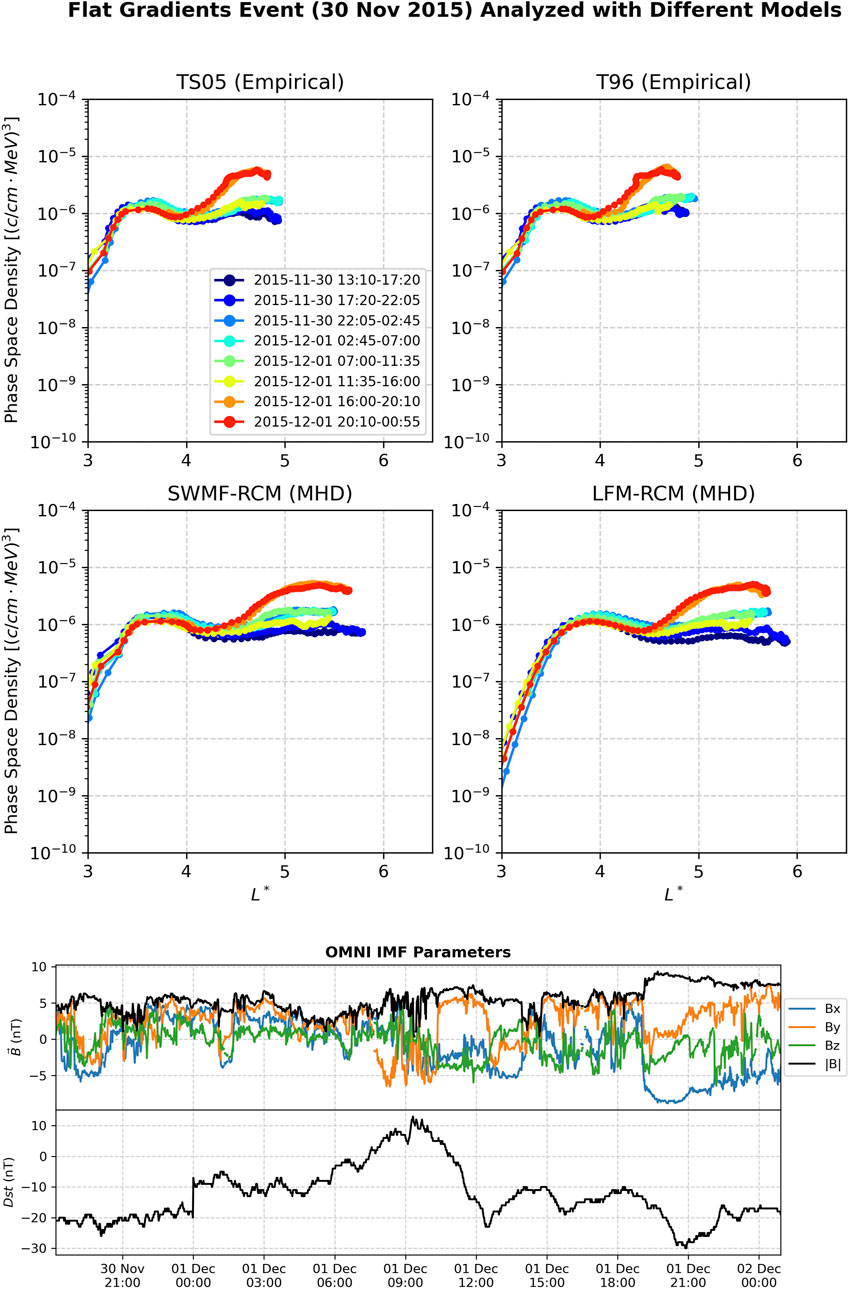
Figure 6. A flat gradients event starting around 30 November, 2015. The phase space density analysis here is performed with four different magnetic field models, and the results from each model largely yield similar interpretations. Magnetic field components are in the GSM coordinate system.
The reprocessing of this event also exhibits model independence in regard to its overall classification. This event is also classified the same way when processed with different models. Again, the Tsyganenko empirical models are closer to each other than they are to the MHD models, and the differences in scale of L* between empirical and MHD models are visible. There are some subtle differences in how slightly negative the slope of f (L*) is in the final line at apogee between the empirical models, but all models show it being slightly negative. While the main growth in f (L*) occurs at the peak of higher L*, there is some growth in the peak of lower L*, and all models show about the same amount of growth, albiet at different L* values. Unlike the growing peak event in Figure 5, this event does not display more gradual increases to f (L*) during the recovery period.
In Figure 7 we process a positive event using the same four models. In Boyd et al. (2018), they note that these can sometimes be revealed to be growing peak events when data at radii beyond the Van Allen Probes apogee are used, such as available through the Time History of Events and Macroscale Interactions during Substorms (THEMIS) mission (Angelopoulos, 2009).
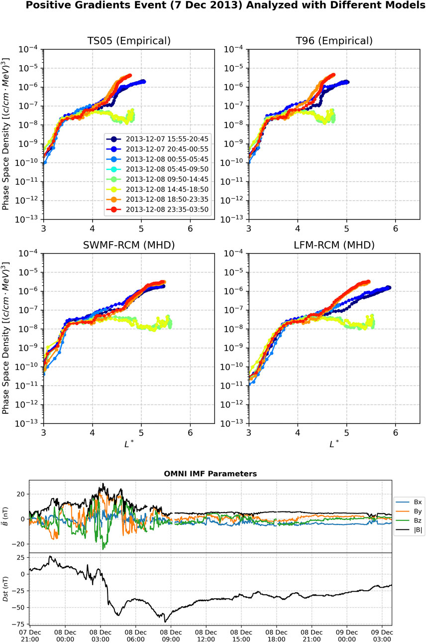
Figure 7. A positive gradients event starting around 7 December, 2015. The phase space density analysis here is performed with four different magnetic field models, and the results from each model largely yield similar interpretations. Magnetic field components are in the GSM coordinate system.
The panels showing the IMF parameters indicate that progression of the Dst index for this storm largely, which follows the conventional pattern for a storm. Clear main phase and a recovery phase are visible, with the nuance that there is a brief interruption in the Dst index recovery around 8 December at 6:00 UT. Like Similar to the flat gradients event previously analyzed, the magnetic field components showed significant variation (this was not the case for the growing peak event previously analyzed). We note that this event is unlike the others in the flat gradients event in that the period of varied magnetic field eventually ceases (around 8 December at 9:00 UT), at which point the magnetic field components become more stable, and the magnetospheric response can be expected to transition towards a steady state.
In this section, we observed that processing the Van Allen Probes data using four magnetic fields models lead to similar classifications of the event type (the classes being growing peaks, flat gradients, and positive gradient types). While the classification remained unchanged, we did notice differences in the scaling of f (L*) between the different models, which implicates conclusions about the particular L* location of individual changes to phase space density. In the SWMF-RCM plot, the first line (dark blue) is much closer in phase space density value to the last line (red), indicating that there was almost no net enhancement between these two times. Should this interpretation be true, this event would not be an enhancement at all.
In this work we study the details of phase space density analysis, wherein one recasts observed flux as phase space density and puts flux in terms of the three adiabatic invariants. Different ways of doing the calculation are presented, with the common ones covered and discussed.
In our analysis of the implementation options, we demonstrated that the interpolation method for j(E) leads to different conclusions as to whether our example event exhibited signatures of internal acceleration or radial transport. In our analysis of the differences to processing our example when |B| from an on-board magnetometer is used over |B| from the magnetic field model, we found that the differences are largely negligible.
This work also studies question of whether, and if so to what extent, the degree to which the identification of signatures from phase space density analyses is dependent depend on the magnetic field model used to do the analysis. We processed three events with four models each, including empirical models TS05 and T96 and coupled MHD simulations SWMF-RCM and LFM-RCM. It was found that each of the interpretations are largely model independent, though some notable differences can be seen in each analysis. These most notable differences are that the MHD models yielded larger values of L* than their empirical counterparts, especially at higher Cartesian radii where the external field dominates. The differences were on the scale of ΔL* = 0.5–1.0 at Van Allen Probe apogee. Within the growing peak event, we also observed a more gradual increase in f (L*) during the recovery of the storm with MHD models, which was distinct from the more sudden increase of f (L*) displayed with the empirical models.
In regards to the question as to whether the magnetic field model used impacts the ability to distinguish local acceleration events from radial transport events, the conclusion of this work is that the analysis is largely overall model independent. It is concluded, however, that use of imprecise implementation options for the steps of calculating f from the observed flux (Figure 1) can lead to major issues, up to and including changing the final result of what acceleration mechanism is identified from the analysis. We therefore recommend that delicate care should be taken in the steps for calculating f, and the implementation option for each step be explicitly stated in the literature.
In this section we address the observation that predictions of L* are systematically larger when MHD models are used (LFM-RCM and SWMF-RCM) over the empirical models used (TS05 and T96). The tendency for L* to be larger in MHD models was previously observed in da Silva et al. (2024), where it was noted that the difference becomes larger further out in the magnetosphere.
The calculation of L* requires calculation of the drift shell. In Figure 8, we show the bounce paths in two drift shells: LFM-RCM (an MHD model) TS05 (an empirical model). In this experiment, the results were computed at increasing radii into the tail for a particle with an equatorial pitch angle of α = 45°. TS05 was evaluated on the LFM grid. In this plot, the bounce paths are plotted in bold colors, with the remainder of the field lines in faded colors.
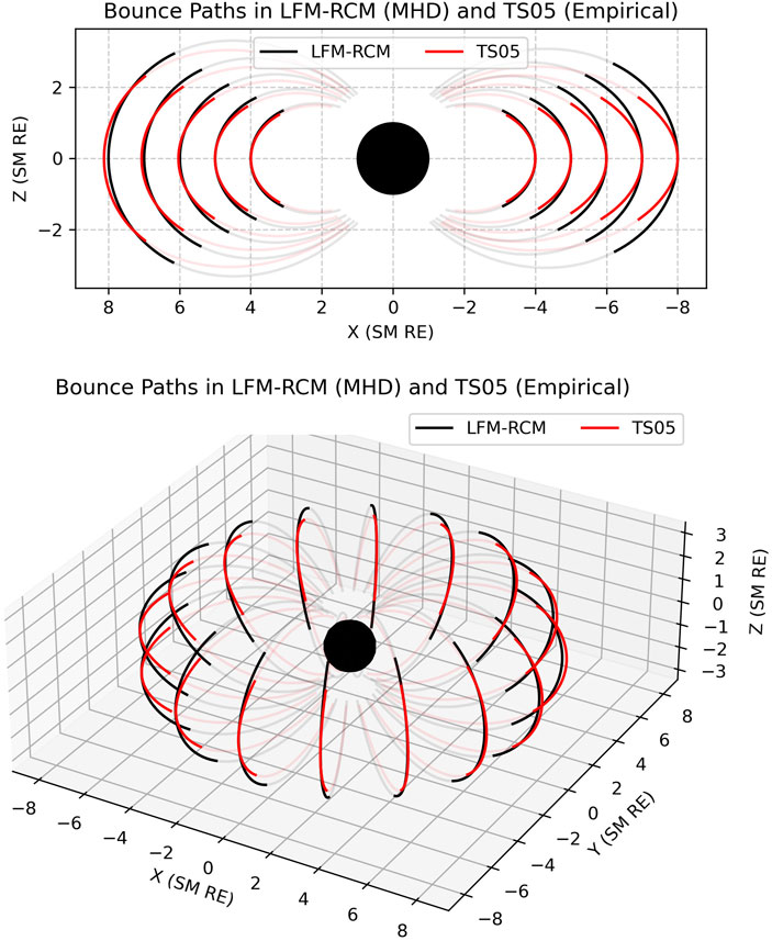
Figure 8. Bounce paths between an MHD model and an empirical model, showing differences in dayside compression and tail stretching. This leads to a different shapes in the polar cap surface Π, which by association changes Φ and L*. Modeling is done for a particle with equatorial pitch angle α =45°.
By definition, L* ∝ 1/Φ where the variable Φ is the magnetic flux through the drift shell (Roederer and Zhang, 2016). The variable Φ is given by
where Π is the polar cap through the drift shell and B is the magnetic field. With the empirical model, we observe increased stretching in the tail and compression on the dayside that alters Π. At each radius considered, the field line of the bounce path with the empirical model stays closer to the equator, and in turns grows the size of the Π surface.
The equation we use for L* is (da Silva et al., 2024)
where Rinner is the inner boundary of the model (2.1 RE in this experiment as TS05 is evaluated on the LFM grid), RE is the radius of the earth, ϕ is the magnetic local time in radians, and θ is the magnetic colatitude of the field line at each magnetic local time at the inner boundary spherical surface. The integral
The differences in the integral
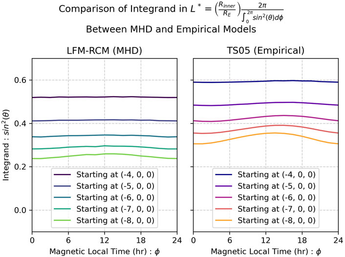
Figure 9. Inspection of the integral embedded in the equation we use for L* (da Silva et al., 2024). This plot inspects the integral between an MHD and empirical model. Calculations are done for a particle with equatorial pitch angle α =45°, with TS05 evaluated on the LFM grid (causing Rinner to be the same).
With these observations we can have confirmed that the polar cap Π in the MHD models is smaller than the MHD models, especially on the day and night sides. From the equations, this leads to decreased Φ and in turn larger L*.
Both empirical and MHD models capture the magnetopause (Chapman-Ferraro) current which flows eastward along the magnetopause and corresponds to compression and increased |B| inside the magnetosphere on the dayside. They also both capture the ring current (to a greater extent when MHD is coupled with RCM as assumed for the MHD models here) which flows westward causing a decrease in |B| in the region typically occupied by outer zone electrons (Kim and Chan, 1997). The degree to which each current system is accurately captured in the statistical ensemble based Tysganenko vs. MHD models determines the relative difference between the two in mapping L*.
Our finding that the MHD models yield a larger value of L* is consistent with a stronger ring current in the MHD-RCM case than found in the empirical models. This has been found to be the case when examining solar energetic proton cutoffs in both types of models for a geomagnetic storm 7–8 September 2017 of comparable magnitude to the three studied here (check). However, these cutoffs are dominated by fields at low L values (3–6). At higher L (and L*) values, magnetopause currents play an increasingly important role. An L − L* comparison for two different geomagnetic storms that IMF Bz, which controls the location of the magnetopause (Shue et al., 1998) and strength of the magnetopause current (Tsyganenko and Sitnov 2005) producing an outward displacement of L* relative to dipole L (r in the equatorial plane) when Bz > 0 and inward displacement when Bz < 0.
Publicly available datasets were analyzed in this study. This data can be found here: https://rbsp-ect.newmexicoconsortium.org/. Software and data used in this study (except for MHD model outputs) can be found at: https://doi.org/10.5281/zenodo.11644307.
DS: Conceptualization, Data curation, Formal Analysis, Investigation, Methodology, Software, Validation, Visualization, Writing–original draft, Writing–review and editing. SE: Conceptualization, Investigation, Supervision, Writing–review and editing. XL: Writing–review and editing. MH: Writing–review and editing. AB: Methodology, Writing–review and editing. AJ: Methodology, Writing–review and editing. MW: Writing–review and editing.
The author(s) declare that financial support was received for the research, authorship, and/or publication of this article. Funding was provided by the NASA FINESST Fellowship.
Author AB was employed by The Aerospace Corporation.
The remaining authors declare that the research was conducted in the absence of any commercial or financial relationships that could be construed as a potential conflict of interest.
All claims expressed in this article are solely those of the authors and do not necessarily represent those of their affiliated organizations, or those of the publisher, the editors and the reviewers. Any product that may be evaluated in this article, or claim that may be made by its manufacturer, is not guaranteed or endorsed by the publisher.
Baker, D. N., Kanekal, S. G., Hoxie, V. C., Batiste, S., Bolton, M., Li, X., et al. (2012). The relativistic electron-proton telescope (rept) instrument on board the radiation belt storm probes (rbsp) spacecraft: characterization of earth’s radiation belt high-energy particle populations. Space Sci. Rev. 179, 337–381. doi:10.1007/s11214-012-9950-9
Blake, J. B., Carranza, P. A., Claudepierre, S. G., Clemmons, J. H., Crain, W. R., Dotan, Y., et al. (2013). The magnetic electron ion spectrometer (mageis) instruments aboard the radiation belt storm probes (rbsp) spacecraft. Space Sci. Rev. 179, 383–421. doi:10.1007/s11214-013-9991-8
Boscher, D., Bourdarie, S., O’Brien, P., Guild, T., Heynderickx, D., Morley, S., et al. (2022) Prbem/irbem: v5.0.0. doi:10.5281/zenodo.6867768
Boyd, A. J., Spence, H., Reeves, G., Funsten, H., Skoug, R. M., Larsen, B. A., et al. (2021). Rbsp-ect combined pitch angle resolved electron flux data product. J. Geophys. Res. Space Phys. 126, e2020JA028637. doi:10.1029/2020ja028637
Boyd, A. J., Spence, H. E., Claudepierre, S., Fennell, J. F., Blake, J., Baker, D., et al. (2014). Quantifying the radiation belt seed population in the 17 march 2013 electron acceleration event. Geophys. Res. Lett. 41, 2275–2281. doi:10.1002/2014gl059626
Boyd, A. J., Turner, D., Reeves, G. D., Spence, H., Baker, D., and Blake, J. (2018). What causes radiation belt enhancements: a survey of the van allen probes era. Geophys. Res. Lett. 45, 5253–5259. doi:10.1029/2018gl077699
Chen, Y., Friedel, R. H. W., and Reeves, G. D. (2006). Phase space density distributions of energetic electrons in the outer radiation belt during two geospace environment modeling inner magnetosphere/storms selected storms. J. Geophys. Res. Space Phys. 111. doi:10.1029/2006ja011703
Chiu, M., Von-Mehlem, U., Willey, C., Betenbaugh, T., Maynard, J., Krein, J., et al. (1998). Ace spacecraft. Space Sci. Rev. 86, 257–284. doi:10.1007/978-94-011-4762-0_13
da Silva, D., Elkington, S. R., Li, X., Murphy, J., Wiltberger, M. J., and Jaynes, A. N. (2022). Tools to calculate adiabatic invariants from dynamic simulations of earth’s magnetosphere. AGU Fall Meet. Abstr. 2022, SM42D–2209. doi:10.1029/2023JA032397
da Silva, D. E., Elkington, S., Li, X., Murphy, J., Hudson, M., Wiltberger, M., et al. (2024). Numerical calculations of adiabatic invariants from mhd-driven magnetic fields. Authorea Prepr. doi:10.3389/fspas.2024.1373019
Elkington, S. R. (2006). A review of ulf interactions with radiation belt electrons. Magnetos. ULF waves Synthesis new Dir. 169, 177–193. doi:10.1029/169gm12
Funsten, H. O., Skoug, R. M., Guthrie, A. A., MacDonald, E., Baldonado, J., Harper, R., et al. (2013). Helium, oxygen, proton, and electron (hope) mass spectrometer for the radiation belt storm probes mission. Space Sci. Rev. 179, 423–484. doi:10.1007/s11214-013-9968-7
Gannon, J., Li, X., and Heynderickx, D. (2007). Pitch angle distribution analysis of radiation belt electrons based on combined release and radiation effects satellite medium electrons a data. J. Geophys. Res. Space Phys. 112. doi:10.1029/2005ja011565
Green, J. C., and Kivelson, M. (2004). Relativistic electrons in the outer radiation belt: differentiating between acceleration mechanisms. J. Geophys. Res. Space Phys. 109. doi:10.1029/2003ja010153
Gu, X., Zhao, Z., Ni, B., Shprits, Y., and Zhou, C. (2011). Statistical analysis of pitch angle distribution of radiation belt energetic electrons near the geostationary orbit: crres observations. J. Geophys. Res. Space Phys. 116. doi:10.1029/2010ja016052
Hartley, D., and Denton, M. (2014). Solving the radiation belt riddle. Astronomy Geophys. 55, 6.17–6.20. doi:10.1093/astrogeo/atu247
Henderson, J. J. N., Morley, M. B., and Walker, A. (2024). drsteve/lanlgeomag: release version 2.2.0-alpha. doi:10.5281/ZENODO.10728854
Heynderickx, D., Quaghebeur, B., Speelman, E., and Daly, E. (2000). ESA’s Space Environment Information System (SPENVIS): a www interface to models of the space environment and its effects. doi:10.2514/6.2000-371
Horne, R. B., Thorne, R. M., Glauert, S. A., Albert, J. M., Meredith, N. P., and Anderson, R. R. (2005). Timescale for radiation belt electron acceleration by whistler mode chorus waves. J. Geophys. Res. Space Phys. 110. doi:10.1029/2004ja010811
Iles, R. H., Meredith, N. P., Fazakerley, A. N., and Horne, R. B. (2006). Phase space density analysis of the outer radiation belt energetic electron dynamics. J. Geophys. Res. Space Phys. 111. doi:10.1029/2005ja011206
Jaynes, A., and Usanova, M. (2019) The dynamic loss of earth’s radiation belts: from loss in the magnetosphere to particle precipitation in the atmosphere. Elsevier.
Kim, H.-J., and Chan, A. A. (1997). Fully adiabatic changes in storm time relativistic electron fluxes. J. Geophys. Res. Space Phys. 102, 22107–22116. doi:10.1029/97ja01814
Kim, H.-J., Kim, K.-C., Noh, S.-J., Lyons, L., Lee, D.-Y., and Choe, W. (2023). New perspective on phase space density analysis for outer radiation belt enhancements: the influence of mev electron injections. Geophys. Res. Lett. 50, e2023GL104614. doi:10.1029/2023gl104614
Kletzing, C., Kurth, W., Acuna, M., MacDowall, R., Torbert, R., Averkamp, T., et al. (2013). The electric and magnetic field instrument suite and integrated science (emfisis) on rbsp. Space Sci. Rev. 179, 127–181. doi:10.1007/978-1-4899-7433-4_5
Kletzing, C. A. (2022). Van allen Probe A fluxgate magnetometer 4 second resolution data in GSM coordinates. doi:10.48322/zrvq-vt55
Konstantinidis, K., and Sarris, T. (2015). Calculations of the integral invariant coordinates <I&gt;I&lt;/I&gt; and <I&gt;L&lt;/I&gt;* in the magnetosphere and mapping of the regions where <I&gt;I&lt;/I&gt; is conserved, using a particle tracer (ptr3D v2.0), LANL*, SPENVIS, and IRBEM. Geosci. Model. Dev. 8, 2967–2975. doi:10.5194/gmd-8-2967-2015
Kruglanski, M., Messios, N., De Donder, E., Gamby, E., Calders, S., Hetey, L., et al. (2009) “Space environment information system (SPENVIS),” in EGU general assembly conference abstracts, 7457.
Lyon, J., Fedder, J., and Mobarry, C. (2004). The lyon–fedder–mobarry (lfm) global mhd magnetospheric simulation code. J. Atmos. Solar-Terrestrial Phys. 66, 1333–1350. doi:10.1016/j.jastp.2004.03.020
Macmillan, S., and Maus, S. (2005). International geomagnetic reference field—the tenth generation. Earth, planets space 57, 1135–1140. doi:10.1186/bf03351896
Ni, B., Zou, Z., Gu, X., Zhou, C., Thorne, R. M., Bortnik, J., et al. (2015). Variability of the pitch angle distribution of radiation belt ultrarelativistic electrons during and following intense geomagnetic storms: van allen probes observations. J. Geophys. Res. Space Phys. 120, 4863–4876. doi:10.1002/2015ja021065
NOAA (2015). G2 (moderate) geomagnetic storms observed on 20 december | noaa/nws space weather prediction center.
Ogilvie, K., Chornay, D., Fritzenreiter, R., Hunsaker, F., Keller, J., Lobell, J., et al. (1995). Swe, a comprehensive plasma instrument for the wind spacecraft. Space Sci. Rev. 71, 55–77. doi:10.1007/bf00751326
Ogilvie, K., and Desch, M. (1997). The wind spacecraft and its early scientific results. Adv. Space Res. 20, 559–568. doi:10.1016/s0273-1177(97)00439-0
Olson, W. P., and Pfitzer, K. A. (1974). A quantitative model of the magnetospheric magnetic field. J. Geophys. Res. 79, 3739–3748. doi:10.1029/ja079i025p03739
Reeves, G., McAdams, K., Friedel, R., and O’brien, T. (2003). Acceleration and loss of relativistic electrons during geomagnetic storms. Geophys. Res. Lett. 30. doi:10.1029/2002gl016513
Reeves, G., Spence, H. E., Henderson, M., Morley, S., Friedel, R., Funsten, H., et al. (2013). Electron acceleration in the heart of the van allen radiation belts. Science 341, 991–994. doi:10.1126/science.1237743
Schulz, M. (1996). Canonical coordinates for radiation-belt modeling. Radiat. Belts Models Stand. 97, 153–160. doi:10.1029/gm097p0153
Selesnick, R., and Kanekal, S. (2009). Variability of the total radiation belt electron content. J. Geophys. Res. Space Phys. 114. doi:10.1029/2008ja013432
Shue, J.-H., Song, P., Russell, C., Steinberg, J., Chao, J., Zastenker, G., et al. (1998). Magnetopause location under extreme solar wind conditions. J. Geophys. Res. Space Phys. 103, 17691–17700. doi:10.1029/98ja01103
Spence, H. E., Reeves, G. D., Baker, D., Blake, J., Bolton, M., Bourdarie, S., et al. (2013). Science goals and overview of the radiation belt storm probes (rbsp) energetic particle, composition, and thermal plasma (ect) suite on nasa’s van allen probes mission. Space Sci. Rev. 179, 311–336. doi:10.1007/s11214-013-0007-5
Thorne, R., Li, W., Ni, B., Ma, Q., Bortnik, J., Chen, L., et al. (2013). Rapid local acceleration of relativistic radiation-belt electrons by magnetospheric chorus. Nature 504, 411–414. doi:10.1038/nature12889
Toffoletto, F., Sazykin, S., Spiro, R., and Wolf, R. (2003). Inner magnetospheric modeling with the rice convection model. Space Sci. Rev. 107, 175–196. doi:10.1007/978-94-007-1069-6_19
Tóth, G., Sokolov, I. V., Gombosi, T. I., Chesney, D. R., Clauer, C. R., De Zeeuw, D. L., et al. (2005). Space weather modeling framework: a new tool for the space science community. J. Geophys. Res. Space Phys. 110. doi:10.1029/2005ja011126
Tsyganenko, N., and Sitnov, M. (2005). Modeling the dynamics of the inner magnetosphere during strong geomagnetic storms. J. Geophys. Res. Space Phys. 110. doi:10.1029/2004ja010798
Tsyganenko, N. A. (1996). Effects of the solar wind conditions in the global magnetospheric configurations as deduced from data-based field models. Int. Conf. substorms 389, 181.
Turner, D., Angelopoulos, V., Li, W., Hartinger, M., Usanova, M., Mann, I., et al. (2013). On the storm-time evolution of relativistic electron phase space density in earth’s outer radiation belt. J. Geophys. Res. Space Phys. 118, 2196–2212. doi:10.1002/jgra.50151
Vampola, A. (1998). “Outer zone energetic electron environment update,” in Conference on the high energy radiation background in space (IEEE), 128–136.
Virtanen, P., Gommers, R., Oliphant, T. E., Haberland, M., Reddy, T., Cournapeau, D., et al. (2020). SciPy 1.0: fundamental algorithms for scientific computing in Python. Nat. methods 17, 261–272. doi:10.1038/s41592-019-0686-2
Zhao, H., Baker, D., Li, X., Jaynes, A., and Kanekal, S. (2018). The acceleration of ultrarelativistic electrons during a small to moderate storm of 21 april 2017. Geophys. Res. Lett. 45, 5818–5825. doi:10.1029/2018gl078582
Keywords: radiation belts, phase space density, adiabatic invariants, geomagnetic storms, magnetospherc physics
Citation: da Silva DE, Elkington SR, Li X, Hudson MK, Boyd AJ, Jaynes AN and Wiltberger M (2024) Radiation belt phase space density: calculation analysis and model dependence. Front. Astron. Space Sci. 11:1423545. doi: 10.3389/fspas.2024.1423545
Received: 26 April 2024; Accepted: 03 June 2024;
Published: 04 July 2024.
Edited by:
Chaoling Tang, Shandong University, ChinaReviewed by:
Si Liu, Changsha University of Science and Technology, ChinaCopyright © 2024 da Silva, Elkington, Li, Hudson, Boyd, Jaynes and Wiltberger. This is an open-access article distributed under the terms of the Creative Commons Attribution License (CC BY). The use, distribution or reproduction in other forums is permitted, provided the original author(s) and the copyright owner(s) are credited and that the original publication in this journal is cited, in accordance with accepted academic practice. No use, distribution or reproduction is permitted which does not comply with these terms.
*Correspondence: D. E. da Silva, ZGFuaWVsLmRhc2lsdmFAbGFzcC5jb2xvcmFkby5lZHU=
Disclaimer: All claims expressed in this article are solely those of the authors and do not necessarily represent those of their affiliated organizations, or those of the publisher, the editors and the reviewers. Any product that may be evaluated in this article or claim that may be made by its manufacturer is not guaranteed or endorsed by the publisher.
Research integrity at Frontiers
Learn more about the work of our research integrity team to safeguard the quality of each article we publish.