Statistical analysis of low latitude spread F at the American, Atlantic, and Pacific sectors using digisonde observations

Statistical analysis of low latitude spread F is presented for three different longitudinal sectors from Jicamarca (12°S, 76.8°W, −2.5° declination angle) from 2001 to 2016, Ascension Island (7.9°S, 14.4°W, −15.09° declination angle) from 2000 to 2014, Kwajalein (8.71°N, 167.7°E, 7.5° declination angle) from 2004 to 2012. Digisonde data from these stations have been processed and analyzed to study statistical variations of equatorial spread F, a diagnostic of irregular plasma structure in the ionosphere. A new automated method of spread F detection using pattern recognition and edge detection for low latitude regions is used to determine solar and seasonal variation over these three sites. An algorithm has been developed to detect the foF2 and hpF2 parameters and this has been validated by comparisons with manually scaled data as well as with SAMI2 and International Reference Ionosphere models showing good correlation. While significant variation is not observed over the solar cycle, the different longitudes and declination angles contribute to the variations over the seasonal cycle.

1 Introduction

Plasma density irregularities in the ionosphere are often observed as a spread pattern in data from radio sounding techniques such as digisondes and are commonly referred to as Spread F. This can be caused by a number of different instability mechanisms, which are controlled in part by the angle of the magnetic field relative to the ionospheric plasma layer. In all cases, the height of the F layer increases before the spread F occurrence (Fejer et al., 1999 and references therein]. Potential mechanisms that influence the growth of spread F include gravity waves (Kil, 2022; Candido et al., 2011; Bowman and Mortimer, 2002; Bowman 2001; Fejer et al., 1999) as well as larger-scale waves (e.g., Takahashi et al., 2021; Aa et al., 2023), and disturbances from geomagnetic storms (e.g., Carter et al., 2014; Cherniak and Zakharenkova, 2022). The various irregularities or spread patterns may be associated with multiple types of plasma structures, such as plumes, patches, bubbles, and blobs (Aarons, 1993). This study focuses on low-latitude regions, where Equatorial Spread F is typically caused by equatorial plasma bubbles (EPBs) that are often observed as spread F plumes in radar echoes. Equatorial spread F has been observed for nearly 80 years (Booker and Wells, 1938), but we are still seeking to understand the physical mechanisms for why it forms on a given night (Carter et al., 2014; Klenzing et al., 2023).

Equatorial spread F has been measured using various instruments such as satellites, ionosondes, scintillation measurements, incoherent scatter radars, rockets and GPS. Afolayan et al. (2019) compared digisonde data for different longitudes to study spread F variation for different solar activities. Gonzalez (2022) used ionosonde and GPS data to study spread F characteristics over Tucuman. Sripathi et al. (2018) used a chain of ionosonde and GPS receivers to study characteristics of equatorial and low latitude plasma irregularities over India. Shi et al. (2011) and Rao et al. (2022a) did correlation studies between spread F from digisonde data and ionospheric scintillations over Hainan, China and Hyderabad, India respectively. Saito and Maruyama [2007] conducted a study of equatorial spread F using ionosondes in south-east Asia. Aarons [1993] did a study of equatorial region sites for 2 years of data. The equatorial electric field pre-reversal enhancement is an essential condition to the development of large-scale irregularities at the equatorial region (Candido et al. 2011, Abadi et al. 2022).

An ionosonde transmits radio waves in a series of varying frequency signals in the ionosphere and receives them back, thereby providing us with the knowledge of density variations present in the ionosphere. The waves are reflected back on Earth when the wave frequency matches the plasma frequency it encounters. The information from the reflected waves, such as time and frequency is used to obtain plots known as ionograms. A smooth, skinny trace on an ionogram will represent a smooth ionosphere while a thick, and a ragged trace will represent disturbances or density irregularities in the ionosphere. This is referred to as the spread condition and is known as spread F when present in the F layer of the ionosphere.

Previous studies on midlatitude spread F by Bhaneja et al. (2009) Bhaneja et al. (2018) determined solar and seasonal cycle variation. The methodology and the algorithm used previously has been modified for these low latitude sites for spread F detection and to determine solar and seasonal cycle variation. The algorithm also detects the F2 layer critical frequency (foF2) and peak height of F2 layer (hpF2) values from an ionogram and this has been validated with comparison with the manually scaled values of foF2 which was done using SAO Explorer: “Interactive ionogram scaling technologies” software created by UMass Lowell and available online. Manual scaling is an important tool for validating the values detected by the algorithms and Rao et al. (2022a) discusses validating the critical layer parameters by manual scaling. Comparisons with Sami2 is another model of the ionosphere (SAMI2) and International Reference Ionosphere (IRI) 2010 models have also been made to validate the algorithm.

Other auto-detection algorithms for detecting spread F have been developed by Lan et al. (2020) with data from Wuhan and Rao et al. (2022a) used CADI data from Hyderabad, India. Lan et al. (2020) defined an automated method using machine learning tools to determine spread F on monograms. Rao et al. (2022a) and Rao et al. (2022b) developed algorithms to detect sporadic E and spread F on ionograms for the CADI instrument data and automatic scaling software respectively. Lynn (2018) used histogram techniques on clean ionograms to develop auto detection for foF2 and h’F2 parameters produced by the IPS5D ionosonde developed and operated by the Australian Space Weather Service (SWS).

Section 2 discusses the ionosonde database and the algorithms used to distinguish between spread and non-spread events. Section 3 presents the statistical results. Section 4 discusses these results for both solar cycles 23 and 24 and the seasonal variation of ESF events. Section 5 summarizes the conclusions and suggests possible future paths of inquiry.

2 Data presentation

The data used in this study has been obtained from digisondes (Digisonde Portable Sounder-4D and DGS 256) at three different low latitude regions; Jicamarca, Ascension Island, and Kwajalein. Figure 1 shows the map with the locations of these stations and Table 1 gives all the detailed information on these sites from latitude, longitude, declination and inclination angles and the years of data processed. This paper uses a previously established pattern recognition algorithm (Bhaneja et al., 2009; Bhaneja et al., 2018) with modifications to automatically detect spread F and determine the foF2 and hpF2 values from ionograms.

Figure 1

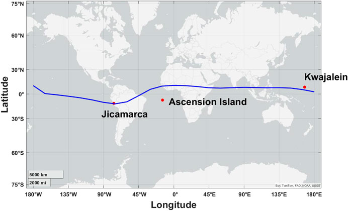
Figure 1. Map showing the location of the three sites globally.

Table 1

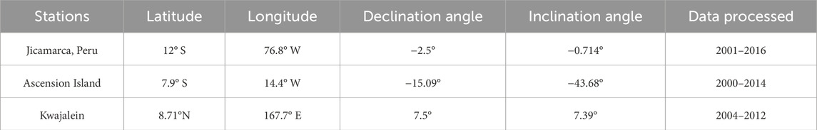
Table 1. Detailed Information for the three stations.

2.1 Spread F

Equatorial spread F is a nighttime phenomenon and thus, the data for nighttime is processed for spread conditions. The measurements taken from the ionosonde include the reflected signal frequency and the time between sending and receiving of the signal. This time is used to calculate the virtual height by using the formula ct/2 where c is the speed of light used for wave travelling in plasma. The plot showing these measurements is called an ionogram. Figure 2A shows an ionogram with a single trace indicating a quiet ionosphere. Figures 2A–D shows three different ionograms with multiple traces or thickness indicating a disturbed ionosphere. Note that there may be multiple traces visible at higher altitudes in the ionograms, which is due to the double reflection of the pulse (from the ionosphere to the ground, back to the ionosphere, and back to the receiver). These second hop traces contain no additional information, and these are ignored in the analysis conducted here.

Figure 2

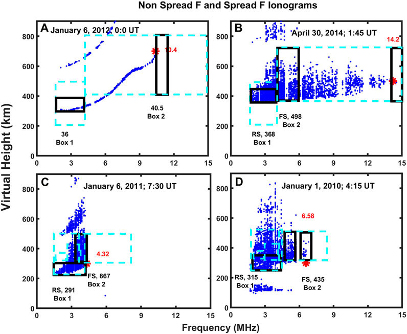
Figure 2. (A) A non-spread F event on 6 January 2012, at 0 UT. Different kinds of Spread F event; (B) Range Spread on 30 April 2014 at 1:45 UT; (C) Range and Frequency Spread on 6 January 2011 at 7:30 UT; (D) Spread in a form of a big blob on 1 January 2010 at 4:15 UT. The left axis is the virtual height in km and the bottom axis is the frequency in MHz. The dotted lines are the boundary boxes and the solid line box is the box selected by the algorithm for determining Range (RS, Box 1tbox1) and Frequency (FS, Box 2tbox2) spread F for an individual ionogram. The corresponding numbers with RS and FS are the pixel counts in each box which determine the spread F. The red star and the corresponding number is the foF2 value determined for the individual ionogram.

Ionogram traces have a finite thickness due to the finite bandwidth of the ionosonde. This is an instrument effect. The thickness or spread indicating spread condition is an ionospheric effect. The equatorial spread F observed on the ionograms generated from Jicamarca data is of three different types: range, range and frequency spread F and spread F in the form of a big blob as observed in Figures 2B–D respectively. Equatorial plasma bubbles or EPBs cause spread F and the ionograms show an extended frequency and flat range spread echoes as shown in Figure 2B (Candido et al., 2011; Sahai et al., 2000). The spread signatures vary from early in the evening 2b with huge plumes and intense spread to 2d with spread reducing later in the evening to 1c where spread signatures are as observed for mid latitude regions later in the night. Range spread F refers to a condition in which there are multiple echoes at different ranges for each frequency. Frequency spreading is the case in which there are multiple echoes at different frequencies around the critical frequency for same height.

There are unusual F region traces as seen in the plots and can be classified into strong, weak and multi trace echo (Saito and Maruyama, 2007). Figures 2B, D refer to the strong spread F where the F region trace is not visible. Afolayan et al. (2019) refers to spread in 2b as strong spread F, while Shi et al. (2011) refers to it as strong range spread F. Weak spread F is where the F region peak is slightly visible as in plot c. These spread events are also defined as bottom-type spread F, bottomside spread F and topside spread F for the 3 different types of spread we see in ionograms (Hysell, 2000; Whalen, 2002; Chapagain et al., 2009). Topside or radar plume goes all the way up and is elongated over F region like plot 2b. This is mostly observed for Jicamarca. High solar flux levels and geomagnetic activity are conducive for the formation of very high-altitude plumes. Plots 2 c and 2 d are also observed at Ascension Island.

Figure 3 shows Range-Time-Intensity (RTI) plot alongside ionograms for three equatorial spread F events. The red line in the RTI plot corresponds to the time of the ionogram. The RTI data has been obtained using JULIA data from Madrigal. All 3 days show radar plumes and corresponding intense spread signatures on the ionograms. The top plot is from October 29–30th night in reference to a rocket launch during midlatitude spread F event observed during a huge hurricane and a high kp observed few hours before midnight (Earle et al., 2010). It is interesting that intense spread signatures are also observed at Jicamarca at the same time. The other two plots also show huge plumes and corresponding intense spread F signatures in the ionograms. Aol et al. (2020) drew similar comparisons observing plasma plumes coinciding with spread F signatures on ionograms between the JULIA radar data and the JRO ionosonde.

Figure 3

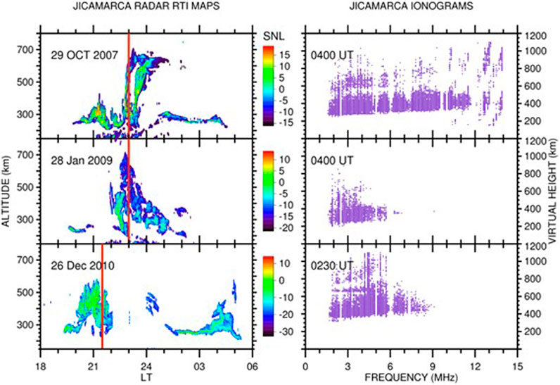
Figure 3. Spread events for 3 days. The (A) shows Range-Time-Intensity plots using JULIA data while the (B) shows ionograms using Jicamarca digisonde data. The red line in the RTI plot corresponds to the time of the ionogram.

2.2 Data analysis-methodology

This study includes data from Jicamarca (2001–2016), Ascension Island (2000–2014) and Kwajalein (2004–2012). Raw digisonde data are available in binary format and has to undergo various data processing steps to obtain ionograms and then identify spread F events and detect foF2 and hpF2 values for statistical analysis. First, the raw data are converted to a text format using the SAO explorer by doing Bulk Processing of ionograms for each day which gives the amplitude echoes of the ionograms. The amplitude threshold in the SAO explorer is set to 6, 8, and 10 for Jicamarca, Ascension Island and Kwajalein respectively to filter out the background noise. The amplitude echoes are then processed using a pattern recognition algorithm for the ordinary mode (O-mode) data because the O-mode does not require knowledge of the magnetic field, therefore it is trivial to incorporate this data into the pattern recognition algorithm.

Figure 2A shows a quiet ionogram where the foF2 can be determined easily. Figures 2B–D shows the spread F identified by two boxes. The heavy spread events like in plots 2b and d, a clear trace is not present and so foF2 cannot be measured accurately for such ionograms. Edge detection is done on both the boxes (solid line boxes) to determine their location; this is done to find the bottom side of box 1 and right side of box 2.

The box 1 (dotted lines) boundary is between 200–500 km and 1.5–4 MHz. The bottom edge for the box is determined by counting the pixels for each altitude starting at 200 km and when the pixel count exceeds 6, the corresponding altitude is chosen as the bottom edge of box 1. The height of this box is fixed at 100 km. Manual inspection of numerous ionograms was conducted to determine the boundaries and heights and widths of the boxes. The limits on the box have been chosen to cover the spread F at night-time while being careful not to include sporadic E and second hop traces.

The height and width of box 2 (dotted lines) is changed for varying ionospheric conditions for the equatorial region as visible on the ionograms. Box 2 has been conditioned for different times of the day; seasons and years; dawn, day, dusk and night; winter and summer season; solar min and solar max years. This has been done to obtain more accuracy for the spread F, foF2 and hpF2 values. The box 2 boundary varies between 400–800 km and 2–15 MHz for dawn, day and dusk times and 300–500 km and 1.2–8 MHz for night times. The right edge for box 2 is determined by counting the pixels for each frequency starting at 6 MHz, and when the pixel count exceeds 6, the corresponding frequency is chosen as the right edge of box 2. Bhaneja et al. (2018), gives the detailed methodology for box 2. Additionally, box 2 was introduced in these plots to obtain a more accurate pixel count for frequency spread F and was taken from the left edge of box 2 with 1.5 MHz width and same height as the boundary box. The average pixel count of both these boxes was taken as the total pixel count for determining frequency spread F. It was necessary as the spread types vary very differently for low latitude regions. The right most edge is taken as foF2 value and is used to determine hpF2_frq = 0.834*foF2. The location of hpF2_frq is hpF2 (UAG, 1972). By assuming a parabolic electron density profile, hpF2 = hmF2 (Bullett, 2012; McNamara, 2008).

The total number of pixel count in the boxes is used to determine the spread condition by comparing it to a set threshold value. These pixel counts are shown in the plots for range spread (RS) and frequency spread (FS) for the two boxes respectively. The pixel counts of 6 for the edges and the thresholds were set by randomly choosing ionograms and checking their threshold counts. Spread events have been quantified, and type of spread is distinguished.

As spread F is a night-time phenomenon, only the data between 7 PM and 7 AM local time is considered. The digisonde produces ionograms every 15 min, 24 h a day. Thus, for our study, around 48 ionograms/night are analyzed. foF2 and hpF2values are however taken for the whole day which is 96 ionograms. A spread event is counted as continuous spread detected across multiple ionograms without interruption of more than 30 minutes (or no more than two ionograms without spread). If more than one event is observed for a night, the longer event is saved and if two equal events are observed the first one is saved for further analysis. On determination of spread F, the onset time, duration, and type of spread F event are recorded and archived for each night. This process is done for the entire set of data. Using this database, statistical analysis is performed to determine seasonal and solar cycle patterns for equatorial spread F. A prototype of a monthly summary plot for July 2011 is shown in Figure 4. The black bars and crosses represent range spread F while the white bars and squares represent frequency spread F. Top panel shows the start time and the second panel shows the duration of spread events for a particular day. The bottom two panels show the foF2 and hpF2 values for each day. The outliers are the values for the noisy and spread ionograms as seen in Figures 2B, D.

Figure 4

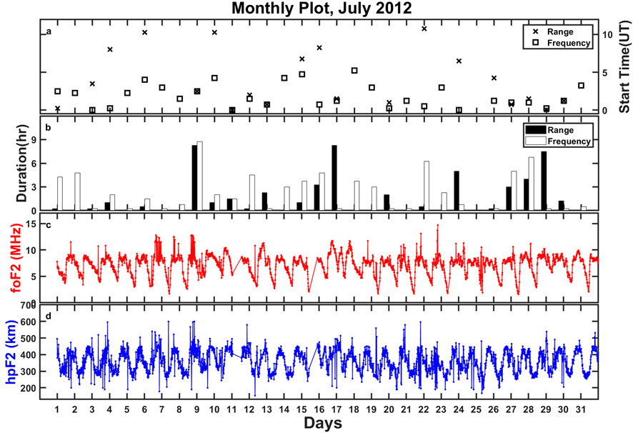
Figure 4. Monthly summary plot for Jicamarca data for July 2011 showing range (black bars) and frequency (white bars) spread F duration and their onset time (cross symbols for range and square symbols for frequency) for night-time hours between 0–10 UT. Panels c and d show the daily foF2 and hpF2 values.

3 Statistical results

Once the daily and monthly plots for spread F were made, the methodology was used towards the entire data set. Figures 5, 6 validates the foF2 detection algorithm by comparisons with manually scaled data and SAMI2 and IRI models values, respectively. Figures 7, 8 show the solar activity variation and Figures 9, 10 show the seasonal variation of equatorial spread F. Figures 11, 12 shows the pre-sunset hpF2 and foF2 vs. spread duration. Figure 13 shows the solar activity variation with spread duration.

Figure 5

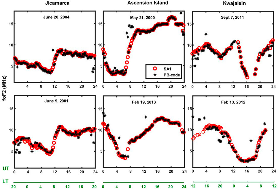
Figure 5. foF2 values plot for an entire day 0–23 UT and corresponding local time (LT) for the three stations. The values shown are algorithm developed (PB-code) in comparison with manually scaled (SA1).

Figure 6

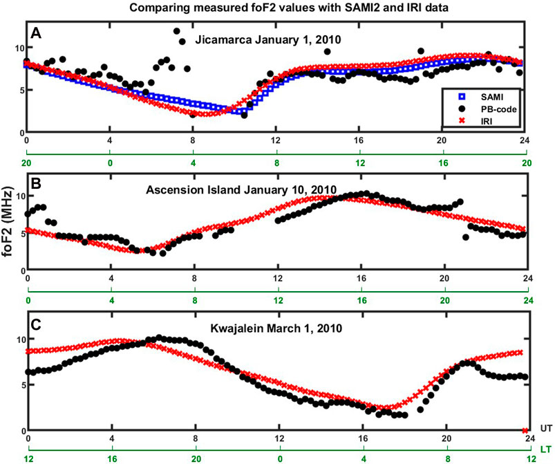
Figure 6. foF2 values plot for an entire day 0–23 UT and corresponding local time (LT) for the three stations. (A) shows comparison of Jicamarca values using the algorithm developed (PB-code) in comparison with both SAMI2 and IRI models. (B,C) show the PB-code values for Ascension Island and Kwajalein respectively in comparison with IRI model values.

Figure 7

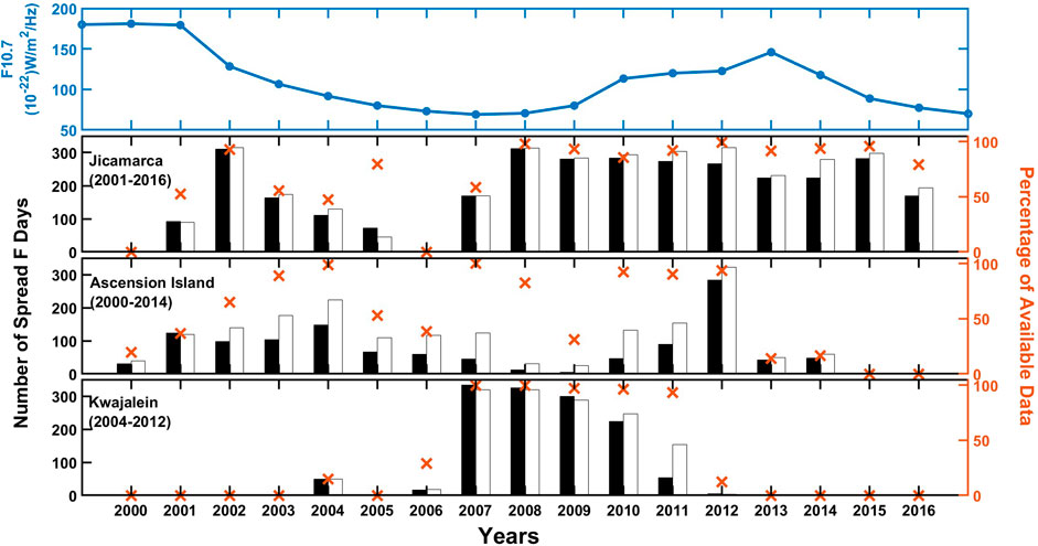
Figure 7. Solar cycle variation of Equatorial Spread F for the three sites from 2000 to 2016 for the available data. The top panel shows the solar flux and the rest three panels show the three sites: Jicamarca, Ascension Island and Kwajalein. The left-hand side shows the number of spread days for range (black bars) and frequency spread F (white bars). The right-hand side shows the percentage of available data (cross symbols).

Figure 8

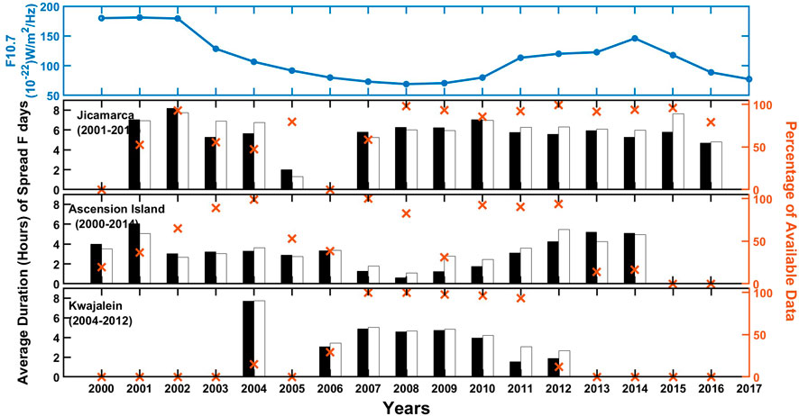
Figure 8. Solar cycle variation of Equatorial Spread F for the three sites from 2000 to 2016 for the available data. The top panel shows the solar flux and the rest three panels show the three sites: Jicamarca, Ascension Island and Kwajalein. The left-hand side shows the average duration (Hours) of spread days for range (black bars) and frequency spread F (white bars). The right-hand side shows the percentage of available data (cross symbols).

Figure 9

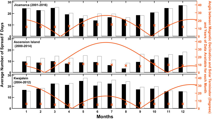
Figure 9. Seasonal cycle variation of Equatorial Spread F for the three sites from 2000 to 2016 for the available data. The panels show the three sites: Jicamarca, Ascension Island and Kwajalein with declination angles of −2.5°, −15.09° and 7.5° respectively. The left-hand side shows the average number of spread days for range (black bars) and frequency spread F (white bars). The right-hand side shows the angle between the declination and the terminator (red line) and the years of data available for each month (cross symbols).

Figure 10

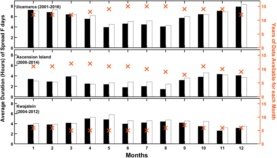
Figure 10. Seasonal cycle variation of Equatorial Spread F for the three sites from 2000 to 2016 for the available data. The panels show the three sites: Jicamarca, Ascension Island and Kwajalein. The left-hand side shows the average duration (Hours) of spread days for range (black bars) and frequency spread F (white bars). The right-hand side shows the years of data available for each month (cross symbols).

Figure 11

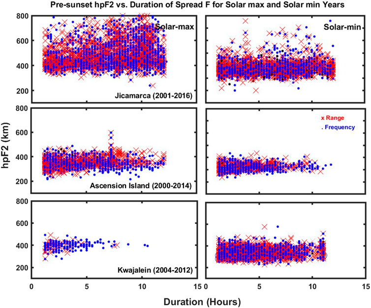
Figure 11. –Pre-sunset variation of hpF2 vs. duration for the three sites in three panels. The (A) shows solar maximum while (B) shows solar minimum. The red cross represents range spread F while blue circles represent frequency spread F.

Figure 12

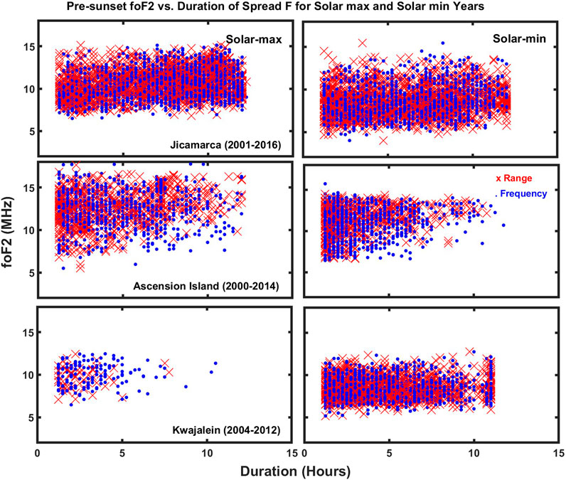
Figure 12. –Pre-sunset variation of foF2 vs. duration for the three sites in three panels. The (A) shows solar maximum while (B) side shows solar minimum. The red cross represents range spread F while blue circles represent frequency spread F.

Figure 13

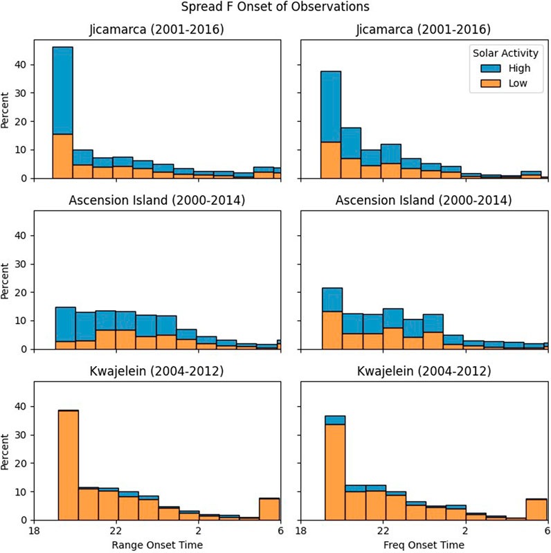
Figure 13. Distribution of Spread-F onset times for observed events versus F10.7 for High Solar Activity (2000–2002, 2011–2015) and Low Solar Activity (2003–2010, 2016) years.

3.1 foF2 comparison with manually scaled values and with SAMI2 and IRI models

Figure 5 shows comparison between the algorithm developed (PB-code) and manually scaled (SA1) values. Random days and years are chosen to show the comparison of the values. The manual scaling of foF2 was done using SAO software created by Lowell. The plots show some values incorrectly detected by the algorithm but with the intense spread F detected in the low latitude regions the detection of F trace is not easy and at times not possible.

Figure 6 shows foF2 values for an entire day (0–23) UT at the three sites. The plots show the PB_code values in comparison with foF2 values as calculated by the IRI model (Bilitza et al., 2014) and the SAMI2 model (Huba et al., 2000; Klenzing et al., 2022). Figure 6A shows comparison of PB_code for Jicamarca data with both SAMI2 and IRI models. Figures 6B, C only show comparison of PB_code for Ascension Island and Kwajalein respectively with IRI model. IRI provides an empirical model of the ionosphere, similar to a monthly average. SAMI2 provides a two-dimensional physical simulation of the ionosphere driven by empirical models of the neutral atmosphere (MSIS, Picone et al, 2002), neutral winds (HWM-14, Drob et al., 2015), and ExB electric fields (Scherliess and Fejer, 1999).

3.2 Solar cycle variation

Figures 7, 8 show the solar cycle variation of spread F for the three sites. The top panel shows the solar flux for all the years covering both solar maximum during 2000–2002 and 2011–2015 and solar minimum during 2003–2010 and 2016. The bottom three panels show the three sites from Jicamarca (2^nd panel), Ascension Island (3^rd panel) and Kwajalein (4^th panel). The right axis shows the percentage of available data represented by the x symbol. Black and white bars represent range and frequency spread F.

Figure 7 shows the number of spread F days for each year of available data between 2000–2016 for Jicamarca, Ascension Island and Kwajalein. The left axis shows the number of spread F days. The ESF events for Jicamarca does not follow any particular pattern for the solar cycle and has spread F events throughout. Ascension Island does not have much spread F during the solar minimum years (2007–2008, 2010). Kwajalein data is only available from 2004 to 2012 and has spread F for almost all those years.

Figure 8 shows the average duration (in hours) of spread F days for each year of available data between 2000–2016 for Jicamarca, Ascension Island and Kwajalein. The left axis shows the average duration of spread F. The total number of longest spread F hours for each month is summed over a given year and then divided by the number of months to obtain average for each year. The average duration of the spread F events for Jicamarca also does not follow any particular pattern and shows long duration events throughout. Ascension Island shows longer duration events during solar maximum years (2001–2002 and 2011–2014). Kwajalein data is only available from 2004 to 2012 and shows longer duration spread F for almost all those years.

3.3 Seasonal cycle variation

Figures 9, 10 show the seasonal cycle variation of spread F for the three sites. The three panels show the three sites from Jicamarca (1^st panel), Ascension Island (2^nd panel) and Kwajalein (3^rd panel). Black and white bars represent range and frequency spread F and the x symbol represents the years of data available for each month.

Figure 9 shows the average number of spread F days for each month for all the years of available data between 2000–2016 for Jicamarca, Ascension Island and Kwajalein along with the angle between declination and terminator. The left axis shows the average number of spread F days for each month for all the available years. The right axis shows the angle along with the years of data available for each month. The average is calculated by first obtaining the sum of spread F nights for each month for each available year. These sums for each year are divided by the number of available years of data to obtain the averages. The red line represents the angle between the magnetic declination and the solar terminator and is plot to compare its variation with spread occurrence around the different seasons. Jicamarca has more spread events during fall and winter months while Kwajalein has more spread for summer months. Ascension Island shows no specific pattern except less spread during July-August months.

Figure 10 shows the average duration (in hours) of spread F for each month for all the years of available data between 2000–2016 for Jicamarca, Ascension Island and Kwajalein. The left axis shows the average number of spread F duration for each month for all the available years. The right axis shows the number of years of data available for each month. The total number of longest spread F hours for each night for each month are counted and then divided by the total number of spread F nights. These monthly averages are then divided by the number of available years of data to obtain the averages. The duration of the spread F events is similar to the occurrence of spread F events; longer duration during fall and winter for Jicamarca and Ascension Island and longer duration during summer for Kwajalein.

3.4 hpF2 and foF2 variation for solar min and solar max

Figures 11, 12 shows the pre-sunset hpF2 and foF2 vs. duration of spread F for all the available data between 2000–2016 for Jicamarca, Ascension Island and Kwajalein. It shows the duration of each spread day versus the pre-sunset hpF2 of that day. The average foF2 and hpF2 for 3 hours from 4–7 PM is obtained for each day and is plotted versus the duration of both types of spread F for that night. It shows how foF2 and hpF2 varies for spread F days for both solar maximum and solar minimum. The three panels show the three sites. The left-hand side shows solar maximum while right-hand side shows solar minimum. The red cross represents range spread F while blue circles represent frequency spread F.

3.5 Solar activity variation

Figure 13 shows the distribution of spread F onset times for all the stations for solar maximum (2000–2002, 2011–2015) and solar minimum (2003–2010, 2016) plotted versus solar local time.

4 Discussion

Figure 1 shows the three low-latitude stations from different longitudinal sectors from which digisonde data was obtained and processed. The different types of spread F for low-latitude regions have been shown in Figure 2. This has also been compared with the Range-Time-Intensity plots using JULIA coherent scatter radar data in Figure 3. The life cycle of spread signatures observed start with huge plumes and intense spread to reduced spread later in the evening down to spread signatures similar to mid latitude spread F characteristics. New methodology has been used to determine spread F characteristics for low latitude sites and to determine solar and seasonal cycle statistical variations for a database spanning more than a decade of data. Figure 4 shows a prototype of monthly plot of spread F, foF2 and hpF2 values.

Comparison and Validation of foF2 data- The data from the detection algorithm has been compared with manually scaled values obtained using the SAO explorer as well as with SAMI2 and IRI models as shown in Figures 5, 6 respectively. The detected values show a good comparison with both manually scaled and model generated values. Both the models provide an average behavior of the ionosphere and are not expected to capture small-scale day-to-day variation. Detailed analysis and further comparisons for validation of foF2 will be addressed in a future paper.

Solar Cycle Variation – It is particularly instructive to compare the rates of ESF at the three sites during the deepest part of the solar minimum (2007–2010). Both Jicamarca and Kwajalein have consistent ESF signatures throughout this period. Ascension Island has low rates of ESF during this time, although the larger dip angle for this site may be the limiting factor, with the ESF events constrained to near the dip equator. For periods of stronger solar activity, we tend to see more frequent ESF events at Ascension Island.

We note that these events are not necessarily all the result of plasma depletion plumes. Candido et al. (2011) observed strong spread F signatures during solar minimum and during solstices June and December months over Cachoeira Paulista in Brazil in the apparent absence of plasma bubbles. The spread F signatures were attributed to medium scale traveling ionospheric disturbances propagating from the mid-latitude region. Similar events are shown in this paper in Figures 2C. The strong range spread F in Figure 2B is associated with equatorial plasma bubbles and is mainly observed during solar maximum years. More plasma bubbles occur during high solar activity during October and March (Sahai et al., 2000). Spread F is mostly consistent throughout solar minimum and maximum and does not show significant change except maybe radar plumes are more observed during solar minimum (Hysell and Burcham, 2002).

Seasonal Variation - The three stations at different longitudes exhibit varying seasonal patterns in Figures 9, 10. For Jicamarca most spread F is observed during months of November to March; Ascension Island during months of September to December; and Kwajalein during months of March to August. This may be due to the local angle of declination. When the terminator aligns with the magnetic field line, both the ends of the tube are in dark, leading to maximum magnetic eastward wind and maximum longitudinal gradient in integrated conductivity. This causes maximum amplitude of pre-reversal enhancement in the vertical drift and therefore maximum irregularity or ESF occurrence. Tsunoda (1985) and Aarons [1993] show similar results with scintillation data. Abdu et al. (1992) mentions how the declination angle affects the sporadic E and F layers. Abdu (2001) discusses similar results with angle of declination and its effects on ESF variation. Afolayan et al. (2019) have similar seasonal variations for Jicamarca and Kwajalein.

An interesting observation from this study and Bhaneja et al. (2018) is that places located at negative declination (Jicamarca and Ascension Island) tend to have most spread F conditions during northern winter seasons (December-February) while places at positive declination (Kwajalein) have most spread F during northern summer seasons (June-August). Jicamarca has similar seasonal pattern as Wallops Island (Bhaneja et al., 2009; Bhaneja et al., 2018), because both Wallops 75.5°and Jicamarca 76.8° are on close longitudes. This suggests that same or close longitude locations have similar spread F occurrence statistics irrespective of their latitude locations. EPBs or Radar Plumes shown in Figure 2B occur more frequently during equinoxes during the low angles for Jicamarca. Burke et al. (2004) analyzed in situ density measurements from DMSP data and found that the EPBs maximize at low angles and mostly occur during April and Aug-Sept periods.

ESF is almost always observed near dusk for all seasons and levels of solar activity and thus we see longer duration of spread F for Jicamarca data. For Jicamarca, less spread F during northern summer (May-August) is observed, probably due to downward drift velocity caused by westward electric field. Evening upward drift velocity and early reversal time causes increase in spread F during equinoxes and Sept-April time. More spread F over Jicamarca is observed between months of September and April and has also been observed by Fejer et al. (1999), Chen et al. (2006), Chapagain et al. (2009) and Aol et al. (2020). During December strong post sunset spread F is observed for Jicamarca. The spread F during the equinox and December months occur mostly during quiet geomagnetic times, and similarly for May-August months (Chapgain et al. 2009). Aarons [1993] observes similar spread F patterns for Kwajalein and Ascension Island. Tsunoda et al. (2015) used satellite and digisonde data and found more spread F during months of May-August for Kwajalein.

foF2 and hpF2 variation - Figures 11, 12 show variation of hpF2 and foF2 for the three stations for spread days for solar minimum and solar maximum years. Saito and Maruyama [2007] observe the variation of hpF2 for spread F events at two stations longitudinally separated by 738 km. They discuss large-scale wave structures as a potential mechanism for the differences in hpF2 between stations. Here we examine stations separated by much longitudinal distances. Potentially, the differences in hpF2 presented here could be modulated by a much larger structure such as a planetary wave [e.g., Liu et al., 2021], although analysis over more longitudinal sectors would be required. Jicamarca has the highest hpF2 for solar maximum for all the three stations. Ascension Island has the highest foF2 of all three stations. Higher foF2 and hpF2 values are observed for the spread F days during solar maximum for all the stations.

Onset time variation – Figure 13 shows the distribution of observed onset times for all three stations in solar local time. Note that onset time here is not necessarily the formation of a plasma plume, but the arrival of the plume at the observatory. Each histogram bin is subdivided into years of high (2000–2002, 2011–2015) and low (2003–2010, 2016) solar activity consistent with the definition elsewhere in this paper. For Jicamarca, the onset times of Range Spread F primarily occurs shortly after dusk during high solar activity, while the onset times are more evenly distributed during low activity. Frequency Spread-F tends to occur later into the night as well. For Ascension Island, both Range and Frequency Spread F are distributed throughout the night, with post-midnight onset times. This may be due in part to the higher magnetic latitude of this station, with plumes forming near the magnetic equator and taking some time to grow large enough to be observed here. Kwajalein shows more frequency spread F for solar min, although we note here that data limitations mean that most of the Kwajelein data occurs during the low solar activity years. High F10.7 contributes to the formation of very high-altitude plumes [Hysell, 2000]. Radar plumes are not observed during solar maximum summer June months.

5 Conclusion

A new method of determining spread F is used to find statistical patterns of equatorial spread F for three sites of Jicamarca, Ascension Island and Kwajalein. The spread F occurs throughout both solar minimum and maximum for all the stations but with varying seasonal patterns. The seasonal patterns vary due to different longitudes and declination angle for the three stations. The onset of Spread-F occurs primarily after sunset at Jicamarca and Kwajalein, but may occur throughout the night at Ascension Island, which is at a higher magnetic latitude. The foF2 values are validated by comparison with manual scaling and with SAMI2 and IRI model values and show good correlation. The algorithm performs well and detects fairly accurate values of the critical frequencies and spread F detection. Future studies will use the spread F detection technique to examine the characteristics of spread F in post-sunset and post-midnight hours over a span of solar cycle under quiet and disturbed space weather conditions.

Data availability statement

The raw data supporting the conclusion of this article will be made available by the authors, without undue reservation.

Author contributions

PB: Conceptualization, Data curation, Formal Analysis, Investigation, Methodology, Project administration, Resources, Software, Supervision, Validation, Visualization, Writing–original draft, Writing–review and editing. JK: Funding acquisition, Supervision, Validation, Visualization, Writing–review and editing. EP: Validation, Writing–review and editing. GE: Supervision, Validation, Visualization, Writing–review and editing. TB: Methodology, Resources, Validation, Visualization, Writing–review and editing.

Funding

The author(s) declare that financial support was received for the research, authorship, and/or publication of this article. Funding is provided by NASA Living With a Star NNH20ZDA001N-LWS.

Conflict of interest

The authors declare that the research was conducted in the absence of any commercial or financial relationships that could be construed as a potential conflict of interest.

Publisher’s note

All claims expressed in this article are solely those of the authors and do not necessarily represent those of their affiliated organizations, or those of the publisher, the editors and the reviewers. Any product that may be evaluated in this article, or claim that may be made by its manufacturer, is not guaranteed or endorsed by the publisher.

Abbreviations

ESF, Equatorial Spread F; EPBs, Equatorial Plasma Bubbles; RTI, Range-Time-Intensity; IRI, International Reference Ionosphere; SAMI2, Sami2 is another model of the ionosphere.

References

Aa, E., Zhang, S.-R., Liu, G., Eastes, R. W., Wang, W., Karan, D. K., et al. (2023). Statistical analysis of equatorial plasma bubbles climatology and multi-day periodicity using GOLD observations. Geo. Res. Lett. 50, e2023GL103510. doi:10.1029/2023GL103510

CrossRef Full Text | Google Scholar

Aarons, J. (1993). The longitudinal morphology of equatorial F-layer irregularities relevant to their occurrence. Space Sci. Rev. 63, 209–243. doi:10.1007/bf00750769

CrossRef Full Text | Google Scholar

Abadi, P., Ahmad, U. A., Otsuka, Y., Jamjareegulgarn, P., Martiningrum, D. R., Faturahman, A., et al. (2022). Modeling post-sunset equatorial spread-F occurrence as a function of evening upward plasma drift using logistic regression, deduced from ionosondes in southeast asia. Remote Sens. 14, 1896. doi:10.3390/rs14081896

CrossRef Full Text | Google Scholar

Abdu, M. A. (2001). Outstanding problems in the equatorial ionosphere-thermosphere electrodynamics relevant to spread F. J. Atmos. Solar-Terres.Phys. 63, 869–884. doi:10.1016/s1364-6826(00)00201-7

CrossRef Full Text | Google Scholar

Abdu, M. A., Batista, I. S., and Sobral, J. H. A. (1992). A new aspect of magnetic declination control of equatorial spread F and F region dynamo. J. Geophys. Res. 97 (A10), 14897–14904. doi:10.1029/92JA00826

CrossRef Full Text | Google Scholar

Afolayan, A. O., Singh, M. J., Abdullah, M., Buhari, S. M., Yokoyama, T., and Supnithi, P. (2019). Observation of seasonal asymmetry in the range spread F occurrence at different longitudes during low and moderate solar activity. Ann. Geophys. 37, 733–745. doi:10.5194/angeo-37-733-2019

CrossRef Full Text | Google Scholar

Aol, S., Buchert, S., Jurua, E., and Milla, M. (2020). Simultaneous ground-based and in situ Swarm observations of equatorial F-region irregularities over Jicamarca. Ann. Geophys. 38, 1063–1080. doi:10.5194/angeo-38-1063-2020

CrossRef Full Text | Google Scholar

Bhaneja, P., Earle, G. D., Bishop, R. L., Bullett, T. W., Mabie, J., and Redmon, R. (2009). A statistical study of midlatitude spread F at Wallops Island, Virginia. J. Geophys. Res. 114, A04301. doi:10.1029/2008JA013212

CrossRef Full Text | Google Scholar

Bhaneja, P., Earle, G. D., and Bullett, T. W. (2018). Statistical analysis of midlatitude spread F using multi-station digisonde observations. J. Atm. Solar-Terres. Phys. 167, 146–155. doi:10.1016/j.jastp.2017.11.016

CrossRef Full Text | Google Scholar

Bilitza, D., Altadill, D., Zhang, Y., Mertens, C., Truhlik, V., Richards, P., et al. (2014). The International Reference Ionosphere 2012 – a model of international collaboration. J. Space Weather Space Clim. 4, A07. doi:10.1051/swsc/2014004

CrossRef Full Text | Google Scholar

Booker, H. G., and Wells, H. W. (1938). Scattering of radio waves by the F-region of the ionosphere. Terr. Magnetism Atmos. Electr. 43 (3), 249–256. doi:10.1029/te043i003p00249

CrossRef Full Text | Google Scholar

Bowman, G. G. (2001). A comparison of nighttime TID characteristics between equatorial-ionospheric-anomaly crest and midlatitude regions, related to spread F occurrence. J.Geophys. Res. 106 (A2), 1761–1769. doi:10.1029/2000ja900123

CrossRef Full Text | Google Scholar

Bowman, G. G., and Mortimer, I. K. (2002). Ionospheric coupling, especially between ionogram-recorded spread-F and sporadic-E enhancements at an equatorial-anomaly crest station, Chung-Li. J. Geophys. Res. 107, A10–A1292. doi:10.1029/2001JA007549

CrossRef Full Text | Google Scholar

Bullett, T. W. (2012). Introduction to ionospheric sounding. Available at: https://indico.ictp.it/event/a13251/session/4/contribution/32/material/0/0.pdf.

Google Scholar

Burke, W. J., Huang, C. Y., Gentile, L. C., and Bauer, L. (2004). Seasonal-longitudinal variability of equatorial plasma bubbles. Ann. Geophys. 22, 3089–3098. doi:10.5194/angeo-22-3089-2004

CrossRef Full Text | Google Scholar

Candido, C. M. N., Batista, I. S., Becker-Guedes, F., Abdu, M. A., Sobral, J. H. A., and Takahashi, H. (2011). Spread F occurrence over a southern anomaly crest location in Brazil during June solstice of solar minimum activity. J. Geophys. Res. 116, A06316. doi:10.1029/2010JA016374

CrossRef Full Text | Google Scholar

Carter, B. A., Yizengaw, E., Retterer, J. M., Francis, M., Terkildsen, M., Marshall, R., et al. (2014). An analysis of the quiet time day-to-day variability in the formation of postsunset equatorial plasma bubbles in the Southeast Asian region. J. Geophys. Res Space Phys. 119 (4), 3206–3223. doi:10.1002/2013JA019570

CrossRef Full Text | Google Scholar

Chapagain, N. P., Fejer, B. G., and Chau, J. L. (2009). Climatology of postsunset equatorial spread F over Jicamarca. J. Geophys. Res. 114, A07307. doi:10.1029/2008JA013911

CrossRef Full Text | Google Scholar

Chen, W. S., Lee, C. C., Liu, J. Y., Chu, F. D., and Reinisch, B. W. (2006). Digisonde spread F and GPS phase fluctuations in the equatorial ionosphere during solar maximum. J. Geophys. Res. 111, A12305. doi:10.1029/2006JA011688

CrossRef Full Text | Google Scholar

Cherniak, I., and Zakharenkova, I. (2022). Development of the storm-induced ionospheric irregularities at equatorial and middle latitudes during the 25–26 August 2018 geomagnetic storm. Space weather. 20, e2021SW002891. doi:10.1029/2021SW002891

CrossRef Full Text | Google Scholar

Drob, D., Emmert, J., Meriwether, J., Makela, J., Doornbos, E., Conde, M., et al. (2015). An update to the Horizontal Wind Model (HWM): the quiet time thermosphere. Earth Space Sci. 2 (7), 301–319. doi:10.1002/2014EA000089

CrossRef Full Text | Google Scholar

Earle, G. D., Bhaneja, P., Roddy, P. A. C. M., Swenson, C. M., Barjatya, A., Bishop, R. L., et al. (2010). A comprehensive rocket and radar study of midlatitude spread F. J. Geophys. Res. 115, A12339. doi:10.1029/2010JA015503

CrossRef Full Text | Google Scholar

Fejer, B. G., Scherliess, L., and de Paula, E. R. (1999). Effects of the vertical plasma drift velocity on the generation and evolution of equatorial spread F. J. Geophys. Res. 104 (A9), 19859–19869. 869. doi:10.1029/1999ja900271

CrossRef Full Text | Google Scholar

Gonzalez, G. (2022). Spread-F characteristics over Tucumán near the southern anomaly crest in South America during the descending phase of solar cycle 24. Adv. Space Res. 69 (3), 1281–1300. doi:10.1016/j.asr.2021.11.009

CrossRef Full Text | Google Scholar

Huba, J. D., Joyce, G., and Fedder, J. A. (2000). Sami2 is Another Model of the Ionosphere (Sami2): a new low-latitude ionosphere model. J. Geophys. Res. Space Phys. 105 (A10), 23,035–23053. 053. doi:10.1029/2000ja000035

CrossRef Full Text | Google Scholar

Hysell, D. L. (2000). An overview and synthesis of plasma irregularities in equatorial spread F. J. Atmos. Phys. 62, 1037–1056. doi:10.1016/s1364-6826(00)00095-x

CrossRef Full Text | Google Scholar

Hysell, D. L., and Burcham, J. D. (2002). Long term studies of equatorial spread F using the JULIA radar at Jicamarca. J. Atmos. Sol-Terr. Phys. 64, 1531–1543. doi:10.1016/s1364-6826(02)00091-3

CrossRef Full Text | Google Scholar

Kil, H. (2022). The occurrence climatology of equatorial plasma bubbles: a review. J. Astron. Sci. 39 (2), 23–33. doi:10.5140/jass.2022.39.2.23

CrossRef Full Text | Google Scholar

Klenzing, J., Halford, A. J., Liu, G., Smith, J. M., Zhang, Y., Zawdie, K., et al. (2023). A system science perspective of the drivers of equatorial plasma bubbles. Front. Astronomy Space Sci. 9, 1–6. doi:10.3389/fspas.2022.1064150

CrossRef Full Text | Google Scholar

Klenzing, J., Smith, J., Hirsch, M., and Burrell, A. G. (2020). Sami2py/Sami2py. Zenodo. doi:10.5281/zenodo.3950564

CrossRef Full Text | Google Scholar

Klenzing, J., Smith, J. M., Halford, A. J., Huba, J. D., and Burrell, A. G. (2022). Sami2py — overview and applications. Front. Astronomy Space Sci. 9, 1–11. doi:10.3389/fspas.2022.1066480

CrossRef Full Text | Google Scholar

Lan, T., Hu, H., Jiang, C., Yang, G., and Zhao, Z. (2020). A comparative study of decision tree, random forest, and convolutional neural network for spread-F identification. Adv. Space Res. 65, 2052–2061. doi:10.1016/j.asr.2020.01.036

CrossRef Full Text | Google Scholar

Liu, G., England, S. L., Lin, C. S., Pedatella, N. M., Klenzing, J. H., Englert, C. R., et al. (2021). Evaluation of atmospheric 3-day waves as a source of day-to-day variation of the ionospheric longitudinal structure. Geophys. Res. Lett. 48, e2021GL094877. doi:10.1029/2021GL094877

PubMed Abstract | CrossRef Full Text | Google Scholar

Lynn, K. J. W. (2018). Histogram-based ionogram displays and their application to auto scaling. Adv. Space Res. 65 (5), 1220–1229. doi:10.1016/j.asr.2017.12.019

CrossRef Full Text | Google Scholar

McNamara, L. F. (2008). Accuracy of models of hmF2 used for long-term trend analyses. Radio Sci. 43, RS2002. doi:10.1029/2007RS003740

CrossRef Full Text | Google Scholar

Picone, J. M., Hedin, A. E., Drob, D. P., and Aikin, A. C. (2002). NRL MSISE-00 empirical model of the atmosphere: statistical comparisons and scientific issues. J. Geophys. Res. 107 (A12), SIA15–16. doi:10.1029/2002JA009430

CrossRef Full Text | Google Scholar

Rao, T. V., Sridhar, M., and Ratnam, D. V. (2022a). An automatic CADI’s ionogram scaling software tool for large ionograms data analytics. IEEE Access 10, 22161–22168. doi:10.1109/ACCESS.2022.3153470

CrossRef Full Text | Google Scholar

Rao, T. V., Sridhar, M., and Ratnam, D. V. (2022b). Auto-detection of sporadic E and spread F events from the digital ionograms. Adv. Space Res. 70 (4), 1142–1152. ISSN 0273-1177. doi:10.1016/j.asr.2022.05.046

CrossRef Full Text | Google Scholar

Sahai, Y., Fagundes, P. R., and Bittencourt, J. A. (2000). Transequatorial F-region ionospheric plasma bubbles: solar cycle effects. J. Atmos. Solar-Terres. Phys. 62, 1377–1383. doi:10.1016/s1364-6826(00)00179-6

CrossRef Full Text | Google Scholar

Saito, S., and Maruyama, T. (2007). Large-scale longitudinal variation in ionospheric height and equatorial spread F occurrences observed by ionosondes. Geophys. Res. Lett. 34, L16109. doi:10.1029/2007GL030618

CrossRef Full Text | Google Scholar

Scherliess, L., and Fejer, B. G. (1999). Radar and satellite global equatorial F region vertical drift model. J. Geophys. Res. Space Phys. 104 (A4), 6829–6842. doi:10.1029/1999JA900025

CrossRef Full Text | Google Scholar

Shi, J., Wang, G., Reinisch, B., Shang, S. P., Wang, X., Zherebotsov, G., et al. (2011). Relationship between strong range spread F and ionospheric scintillations observed in Hainan from 2003 to 2007. J. Geophys. Res. Space Phys. 116, 1–5. doi:10.1029/2011JA016806

CrossRef Full Text | Google Scholar

Sripathi, S., Sreekumar, S., and Banola, S. (2018). Characteristics of equatorial and low-latitude plasma irregularities as investigated using a meridional chain of radio experiments over India. J. Geophys. Res. Space Phys. 123, 4364–4380. doi:10.1029/2017JA024980

CrossRef Full Text | Google Scholar

Takahashi, H., Essien, P., Figueiredo, C. A. O. B., Wrasse, C. M., Barros, D., Abdu, M. A., et al. (2021). Multi-instrument study of longitudinal -12wave structures for plasma bubble seeding in the equatorial ionosphere. Earth Planet. Phys. 5 (5), 368–377. eepp2021047. doi:10.26464/epp2021047

CrossRef Full Text | Google Scholar

Tsunoda, R. T. (1985). Control of the seasonal and longitudinal occurrence of equatorial scintillations by the longitudinal gradient in integrated E region Pedersen conductivity. J. Geophys. Res. 90 (A1), 447–456. doi:10.1029/ja090ia01p00447

CrossRef Full Text | Google Scholar

Tsunoda, R. T., Nguyen, T. T., and Le, M. H. (2015). Effects of tidal forcing, conductivity gradient, and active seeding on the climatology of equatorial spread F over Kwajalein. J. Geophys. Res. Space Phys. 120, 632–653. doi:10.1002/2014JA020762

CrossRef Full Text | Google Scholar

UAG (1972). “World data center a for solar-terrestrial physics,” in URSI handbook of ionogram interpretation and reduction. 2nd Edn. Available at: https://data.ngdc.noaa.gov/instruments/remote-sensing/active/profilers-sounders/ionosonde/documentation/UAG_23A_Searchable.pdf/.

Google Scholar

Whalen, J. A. (2002). Dependence of equatorial bubbles and bottomside spread F on season, magnetic activity, and E × B drift velocity during solar maximum. J. Geophys. Res. 107, A2–A1024. doi:10.1029/2001JA000039

CrossRef Full Text | Google Scholar