Prediction of ionospheric TEC during the occurrence of earthquakes in Indonesia using ARMA and CoK models

Predicting ionospheric Total Electron Content (TEC) variations associated with seismic activity is crucial for mitigating potential disruptions in communication networks, particularly during earthquakes. This research investigates applying two modelling techniques, Autoregressive Moving Average (ARMA) and Cokriging (CoK) based models to forecast ionospheric TEC changes linked to seismic events in Indonesia. The study focuses on two significant earthquakes: the December 2004 Sumatra earthquake and the August 2012 Sulawesi earthquake. GPS TEC data from a BAKO station near Indonesia and solar and geomagnetic data were utilized to assess the causes of TEC variations. The December 2004 Sumatra earthquake, registering a magnitude of 9.1–9.3, exhibited notable TEC variations 5 days before the event. Analysis revealed that the TEC variations were weakly linked to solar and geomagnetic activities. Both ARMA and CoK models were employed to predict TEC variations during the Earthquakes. The ARMA model demonstrated a maximum TEC prediction of 50.92 TECU and a Root Mean Square Error (RMSE) value of 6.15, while the CoK model predicted a maximum TEC of 50.68 TECU with an RMSE value of 6.14. The August 2012 Sulawesi earthquake having a magnitude of 6.6, revealed TEC anomalies 6 days before the event. For both the Sumatra and Sulawesi earthquakes, the GPS TEC variations showed weak associations with solar and geomagnetic activities but stronger correlations with the earthquake-induced electric field for the considered two stations. The ARMA model predicted a maximum TEC of 54.43 TECU with an RMSE of 3.05, while the CoK model predicted a maximum TEC of 52.90 TECU with an RMSE of 7.35. Evaluation metrics including RMSE, Mean Absolute Deviation (MAD), Relative Error, and Normalized RMSE (NRMSE) were employed to assess the accuracy and reliability of the prediction models. The results indicated that while both models captured the general trend in TEC variations, nuances emerged in their responses to seismic events. The ARMA model demonstrated heightened sensitivity to seismic disturbances, particularly evident on the day of the earthquake, whereas the CoK model exhibited more consistent performance across pre- and post-earthquake periods.

1 Introduction

The ionosphere plays a focal role in the propagation of radio signals and communication systems. Understanding its behaviour, especially during seismic events like earthquakes, is of paramount importance for mitigating potential disruptions in communication networks. The Ionosphere is divided into four layers D, E, F₁, and F₂. The particles present in the Ionospheric layer are ionized due to solar activity and other factors. Due to ionization, the free electrons will increase in the region. Total Electron Content (TEC) is the count of charged free electrons particles scattered all over the atmosphere. Other than solar activity, seismic activity in the lithospheric region of the earth causes high-pressure air to be released into the atmosphere which causes an increase in the TEC value. This phenomenon is called as positive hall effect. In this research, we have attempted to predict the Ionospheric TEC changes above the Indonesian region during earthquake events. Figure 1 shows the location of the epicentre of the earthquake and BAKO station.

Figure 1

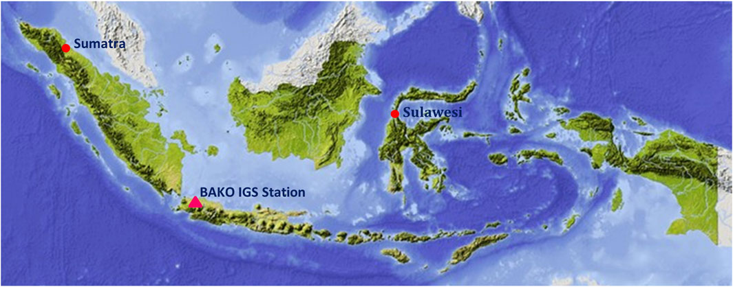
Figure 1. Location of Epicentre of earthquakes (Red dots) and BAKO IGS station (Red triangle).

For the benefit of human life, satellites were launched and placed in the region outside of the atmosphere of Earth. These satellites help in many ways but one of the very effective and useful fields is navigation. The leading navigation systems of the world are affected by TEC variations. If a higher amount of TEC is present in a particular region, the increased TEC causes errors in the signals that are transmitted through the Ionosphere. This error causes a delay in the delivery of signals at the required time which is commonly referred to as Ionospheric Time Delay (ITD). The seismo-ionospheric phenomena are considered to be a result of the lithosphere–atmosphere–ionosphere coupling and a signal of the forthcoming earthquake. The seismic ionospheric effect is shown in Figure 2.

Figure 2

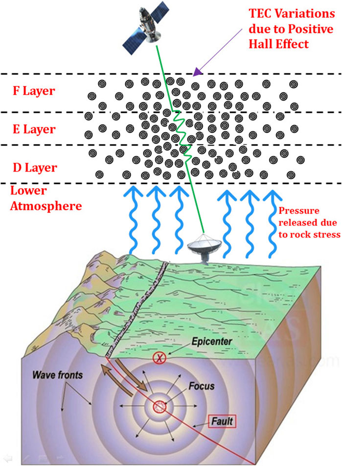
Figure 2. Seismo-ionospheric phenomenon.

A connection between earthquakes and the ionosphere has been proposed by several researchers. Theories suggest that faults release electrical energy in the days leading up to an earthquake. The hypothesis on the possible internal or acoustic gravity wave generation before earthquakes was proposed by many authors. Acoustic gravity waves are said to be a possible source of the disturbances observed in the ionosphere before strong earthquakes and as a mechanism of seismo-ionospheric coupling. Research has shown that the value of TEC is usually lowest at midnight and before sunrise and highest in the afternoon. But in the case of any activities which affect TEC, the TEC variations are shown unnaturally. Such kinds of activities often show some kind of pattern from the past and if examined systematically then the value of TEC could be predicted a few days ago. The aim of the study is that if the TEC could be predicted even 1 day ahead of the erratic events occurring then the positional accuracy of the satellite signals could be increased drastically henceforth enhancing the accuracy of navigation and also it will be useful for safeguarding the people from EQ if the ionospheric variations happened due to EQ. Rigorous study is done in the field of ionospheric modelling to develop the most suitable prediction model. The literature survey on recent developments in this field is essential to understand the efficiency of different models under different conditions. Some of the literatures that discuss similar types of research are given in this section.

Akyol et al. (2020) address the challenging task of earthquake prediction, focusing on the detection of precursory signals using ionospheric data and Earthquake Precursor Detection technique (EQ-PD). The EQ-PD technique proposed in this study leverages support vector machine (SVM) classification to identify spatiotemporal anomalies in ionospheric data that may indicate earthquake precursors. The performance of the EQ-PD technique is evaluated over a region covering Italy during a specified period, demonstrating its ability to detect precursors for earthquakes with magnitudes above four on the Richter scale. The paper discusses the physical mechanisms underlying ionospheric anomalies preceding earthquakes, including the Lithosphere-Atmosphere-Ionosphere Coupling (LAIC) model, which suggests a connection between seismic activity and ionospheric disturbances caused by phenomena like radon gas emissions. The study conducted by Muhammad et al. (2023) investigates the interplay between seismic activity, radon gas, and ionospheric TEC to shed light on the LAIC phenomenon. By analyzing data from the North Anatolian Fault (NAF) region between 2007 and 2009, the researchers employed statistical and machine/deep learning methods like ARIMA, LSTMs, ANNs, SVMs, and STUMPY to explore potential correlations and anomalies. By analyzing earthquakes with magnitudes ranging from 4.0 to 5.0, the researchers identified instances where Rn anomalies were deemed seismically induced based on specific criteria related to the earthquake preparation radius.

Maltseva and Mozhaeva (2016) explained that the Local, regional and global model can be created using the TEC data to correct the ionospheric delay by increasing the accuracy of positioning. In this paper, the analysis of investigation, utilization of Equivalent Slab Thickness of the ionosphere and construction of the Emperial model is attempted. Venkata Ratnam and Sarma (2012) developed a spherical harmonic-based ionospheric delay model by considering data from 17 GAGAN TEC stations and IGP delay variations are estimated and investigated for quiet and disturbed days over the Indian region. It is observed that delays are more during the autumn equinox compared to the summer season. SHF model is compared with other standard models. Hence, these techniques could be considered in satellite-based navigation systems for better accuracy. Liu et al. (2022) implemented the Four convolutional long short-term memory (convLSTM)-based ML algorithms to predict daily global TEC maps using CODE data that maps with up to 24 h of lead time at a 1-h interval over a period of nearly 7 years. Huang and Yuan (2014) developed an RBF neural network improved by the Gaussian Mixture Model for forecasting ionospheric 30 min TEC. Data obtained from ground stations at different latitudes are pre-processed which can lead to good prediction. Comparison with the BP network indicates that the RBF network offers a powerful and reliable tool for the design of ionospheric TEC forecasts.

Han et al. (2022) discussed the use of machine learning models like artificial neural networks, long short-term memory networks, adaptive neuro-fuzzy inference systems and GBDT for forecasting TEC. Three IGS stations at low latitude regions were considered and data from 2012–2015 were used for the study. SZA, F10.7, Dst, Kp, and TEC values were the five features used for the machine-learning-based algorithm. The training dataset is from 2012 to 2014 and the testing dataset is from the year 2015. It was observed that the new GBDT gives the best results out of the four models. It was also observed that during varying space weather, machine-learning-based methods performed better than the standard model like IRI-2016. Cander (1998) explained the use of artificial neural networks to model and predict the variations of TEC and f₀F₂ at mid-latitude ionosphere during different solar and geomagnetic conditions. Faraday rotation observations at Florence using the signal of the OTS-2 satellite were used to determine the TEC data. The modified f₀F₂ neural network forecasting model was used to introduce the TEC prediction 1 h ahead. The results show that the data obtained from neural networks agree with the actual data most times, but some discrepancies were observed. Tang et al. (2022) used Machine machine-learning model for the prediction of global ionospheric TEC. Harmonic coefficients are used for calculations. The prediction is done using sets of data of 15 and 30 days. The results provided by the model are good for both the high and low solar activity periods. Sur et al. (2015) did research on the equatorial region, where the TEC values are high and much volatile. Three artificial neural network models are developed for real-time low-latitude TEC data. It predicts more accurate VTEC than standard models like IRI, Parameterized Ionospheric Model, and NeQuick as the neutral wind effects are used as input for the ANN model. Tebabal et al. (2018) discussed the model used for TEC prediction constructed based on neural networks where solar and geomagnetic parameters were taken into account. The value of TEC is taken from GPS mid- and low-latitude stations from the years 2011 to 2014. The Model predicted well in low latitudes and 1 day ahead prediction can be done.

Sivavaraprasad et al. (2020) explained the performance of TEC forecasting models based on Neural Networks (NN). The NN has been trained and evaluated over equatorial low latitude Bengaluru, India for 7 years (2009–2015). The performance of NN-based TEC forecast models and International Reference Ionosphere, IRI- 2016 global TEC model has been evaluated during the testing period, 2016. The NN-based model (NNunq) driven by all the inputs has shown better accuracy. Draz et al. (2023) investigated the changes in the atmospheric parameters and ionospheric TEC during the 13.2.2021 Japan Earthquake. Wavelet, ANN, NARX, and LSTM methods were used to predict the anomalies based on the data obtained from the HYDE, USUD, and MTKA stations. The results show the importance of machine learning techniques for detecting the anomalies related to the earthquake. Mukesh et al. (2024) predicted TEC using RNN during 10 earthquakes that happened in Indonesia region from 2004 to 2024. The RNN model was trained with the data obtained from the IGS BAKO station. The predicted results were compared with the IRI-2020 model and the comparison analysis shows that the RNN model performed well during the considered periods. Reddybattula et al. (2022) applied the LSTM model for forecasting TEC during the 24th solar cycle. 8 years (2009–2017) of GPS TEC data obtained from the IISC station were utilized for training and validation of the model. The TEC predicted results during the year 2018 were compared with the IRI 2016 model. The results show that the LSTM model performed well when compared with the IRI model. Vankadara et al. (2023) forecasted the TEC during quiet and disturbed days using Bi-LSTM based on the data obtained from the KLEF campus. The forecasted results were compared with the LSTM, ARIMA, IRI-2020, and GIMs. The results show that Bi-LSTM performed well when compared to the other models. Apart from that, Bi-LSTM prediction capability is also verified with IISC station results. Maheswaran et al. (2024) predicted VTEC over Thanjavur GPS station by using Bi-LSTM. The Deep learning model was trained with solar and geomagnetic parameters for the prediction of TEC during solstice and equinox periods. Statistical parameters like MAE, MSE, and RMSE were used to analyze the performance of the model. The results show that Bi-LSTM produced good results when compared to the LSTM model.

The authors analyzed the TEC variations that happened before the Baja California Earthquake (EQ). GPS TEC data were collected from six IGS stations. The results show that EQ-related TEC variations occurred before the EQ event (Ulukavak and Yalcinkaya, 2016). Nayak et al. (2023) used the crustal stress (b) values along with the TEC as a precursor for the detection of EQ that occurred in Mexico on 19.9.2022. The results show that TEC anomalies were found before the EQ and also it reveals that whenever the b values were less, the TEC values also reduced. The author discussed the effects on the ionosphere during the 2004 EQ that occurred in Indonesia based on the data obtained from the IRI model. The results revealed that the anomaly was caused 1 day before the EQ (Koklu, 2023). Ke et al. (2015) analyzed the TEC variations during EQs that happened during the years from 2003 to 2013 over China based on the TEC data obtained from the IGS network. TEC variations for 20 days before and after the EQs were analyzed, and the results show that anomalies were found before the EQs. The authors used the sliding interquartile range method for analyzing the variations of TEC before the April 2014 EQ occurred in Chile. Positive TEC anomalies were found before the EQ which was due to the electric fields produced in the EQ preparation area (Jiang et al., 2017).

Saqib et al. (2021) used the ARIMA method to predict TEC anomalies during the EQs that occurred in India and Turkey. The result shows that the developed model detects the anomalies well. Thomas et al. (2022) used three stations GPS TEC values to analyze the seismo-ionospheric anomalies by using statistical techniques before the Haiti EQ which happened on 14.8.2021. The results revealed that 82% of anomalies were related to EQ. Another study investigates earthquake precursors in the Himalayan region, focusing on ionospheric perturbations using GNSS data analyzed through IONOLAB-TEC. The study examines TEC data from 15 GNSS stations before five random Himalayan earthquakes, employing IONOLAB-TEC with a 30-s temporal resolution. Selected earthquakes include the 2015 Nepal quake (Mw 7.3) and the 2020 Manipur quake (Mw 5.2). The study area encompasses various lithologies, faults, and fractures, contributing to seismic activity. Analysis of GNSS data revealed TEC anomalies preceding the earthquakes by up to a month, followed by perturbations in the earthquake preparation zones (Joshi et al., 2023).

Research by Sergey Pulinets (2004) provides a comprehensive overview of recent advancements in understanding seismo-ionospheric coupling and its practical implications for earthquake prediction. The paper discusses how anomalous electric fields penetrate the ionosphere, creating irregularities and disturbances in electron concentrations. These disturbances manifest as sporadic E-layers and large-scale irregularities in the F2 region, observable through satellite and ground-based monitoring. Zhu et al. (2018) focuses on the statistical analysis of ionospheric TEC anomalies preceding large earthquakes with magnitudes greater than or equal to 6.0. Covering the period from 2003 to 2014, the researchers aim to investigate whether there are differences in the morphological characteristics of TEC anomalies between daytime and night-time before seismic events. Using data from the global ionosphere map (GIM), the study examines the spatial-temporal distribution of TEC anomalies before and during M6.0+ earthquakes worldwide. The findings indicate that apart from a higher occurrence rate of pre-earthquake ionospheric anomalies (PEIAs) at night compared to daytime, there are no statistically significant differences in the spatial-temporal distribution of PEIAs between the two time periods. Another research by Zhu et al. (2023) provides a thorough examination of the accuracy of the GIM in China. The study utilizes high-precision Regional Ionospheric Maps (RIMs) based on Crustal Movement Observation Network of China (CMONOC) GNSS data as reference values for comparison with the IGS GIM. This approach allows for a detailed assessment of the actual accuracy of the GIM over the China region, which is particularly important given the dense and continuous GNSS network in China and its high seismic activity. Statistical measures such as RMS, bias, and standard deviation are employed to assess the accuracy of the GIM. The results indicate that the average RMS of the GIM over China is less than 2 TECu, and the bias and STD of the difference between the GIM and RIM are generally within 2 TECu, except for some low latitude areas. After a thorough study of the literature, this research work uses the ARMA and CoK models to predict TEC during the Earthquake that happened in Indonesia during the years 2004 and 2021.

2 Methodology

This section explains the method of approach incorporated in this work. The flow chart for the methodology employed in forecasting TEC for the Earthquake-prone region of Indonesia is shown in Figure 3.

Figure 3

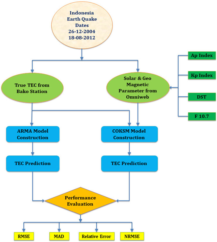
Figure 3. Prediction of TEC over Indonesia using ARMA and COKSM.

In this paper, the GPS TEC data, and the forecast TEC data for 8 days are considered for the analysis of model performance. The GPS TEC data is obtained from the IONOLAB website (http://www.ionolab.org/) for the low latitude BAKO station, Indonesia which is located at −6.45˚N and 106.85˚E. The BAKO station belongs to the International GNSS Service. IONOLAB provides robust, automatic and near-real-time TEC for the IGS stations. IONOLAB developed a novel automatic routine for checking the pseudorange and phase delay values. The cycle slips were corrected by using a special algorithm and also inter-frequency receiver bias was computed by the IONOLAB-BIAS routine. The TEC values were estimated from pre-processed RINEX files. The estimated TEC provided by IONOLAB is accurate and reliable (Sezen et al., 2013). Geomagnetic and Solar indices were taken from the OMNIWEB DATA server [https://omniweb.gsfc.nasa.gov]. The GPS TEC data from 30 days before the prediction day is fed to the ARMA model as training data to obtain the TEC forecast. The GPS TEC data, geomagnetic parameters like Planetary K and A indices (Kp and Ap), Disturbance Storm Time (DST) index and solar parameter Radio Flux at 10.7 cm (F10.7) of 6 days before the prediction day is fed to the CoK model as training data to obtain the TEC forecast. The Auto Regressive Moving Average (ARMA) model combines Auto Regression (AR) and Moving Average (MA) methods for time series forecasting (Ratnam et al., 2019). AR models involve a time-varying process where output variables exhibit linear correlation with lagged observations through coefficients (φ), while MA models express the current value as a linear combination of the mean (c) and past error terms (ε) with coefficients (θ) indicating the impact of past errors on the current value. An ARMA model integrates both past observations and past innovations, denoted as ARMA (x,y), where “x” represents the AR degree and “y” is the MA degree. The form of the ARMA (x,y) model is given in Equation 1.

$F_t=c+{\phi }_1{F}_{t-1}+......+{\phi }_x{F}_{t-x}+{\epsilon }_t+{\theta }_1{\epsilon }_{t-1}+......+{\theta }_y{\epsilon }_{t-y}(1)$

where ${\epsilon }_t$ is an uncorrelated innovation process with mean zero.

Cokriging is a method that uses two sets of related data to predict values at specific points. Combining cokriging with surrogate modelling yields a cokriging-based surrogate model suitable for Total Electron Content (TEC) prediction (Mukesh et al., 2020). This model utilizes 6 days of past data collected at various resolutions to predict TEC for a given day, employing a multivariate system with matrix cross-semi variogram operators. The Cokriging-based Surrogate Model (CoK) algorithm, as described, employs weighted parameters (λ) to distribute between primary (m) and secondary (n) variables, where primary variables are essential for TEC prediction and secondary variables include Kp index, Ap index, F10.7 radio-flux, DST index and equivalent TEC values. The algorithm utilizes cross-correlated data (Y variable) to minimize prediction errors and is implemented in MATLAB software. (Mukesh et al., 2020). The governing mathematical formula for CoK is given in Equation 2.

${\mathrm{\Lambda }}^{*}\left(x_p\right)={\displaystyle {\sum }_{i=1}^m}{\lambda }_i\mathrm{\Lambda }\left(x_i\right)+{\displaystyle {\sum }_{j=1}^n}{\lambda }_j^{`}.\mathrm{\Psi }\left(x_j^{`}\right)(2)$

whereas $\lambda$ is the weight parameters distributed between primary (m) and secondary (n) variables of order (i, j) and $\mathrm{\Lambda }$^* (x_p) is the predicted value at location x_p.

3 Results and discussion

Accurately predicting ionospheric changes before earthquakes is vital for effective communication during disasters. To forecast TEC variations, models like ARMA and CoK are used. Evaluating how well these models perform is crucial to ensure dependable predictions and improve our grasp of how the ionosphere reacts to seismic events. The performance metrics used in the study offer numerical assessments of the models’ precision, reliability, balance in prediction errors, and the degree of linear associations between predicted and actual TEC values. Root Mean Square Error (RMSE), Mean Absolute Deviation (MAD), Relative Error, and Normalized Root Mean Square Error (NRMSE) are common performance metrics used to evaluate the accuracy of predictive models. RMSE is a measure of the differences between predicted values and observed values. It calculates the square root of the average of the squared differences between predicted and observed values. RMSE provides a measure of the typical magnitude of the prediction errors without considering the direction of the errors. It is calculated using the formula. Mean Absolute Deviation measures the average absolute differences between predicted and observed values. It provides a more robust measure of prediction accuracy compared to RMSE as it is less sensitive to outliers. MAD is calculated as the average of the absolute differences between predicted and observed values. Relative Error (${\mathit{E}}_{\mathit{r}\mathit{e}\mathit{l}}$) is a measure of the prediction error relative to the magnitude of the observed values. It is calculated as the ratio of the absolute difference between predicted and observed values to the observed value. Normalized Root Mean Square Error is a standardized version of RMSE, which accounts for the scale of the observed values. It is calculated by dividing the RMSE by the range of the observed values. RMSE, MAD, Relative Error, and NRMSE are important metrics for assessing the accuracy and reliability of predictive models, providing insights into the magnitude and direction of prediction errors relative to the observed values. The mathematical formula for the statistical parameters is given in Equations 3–6.

$\mathbf{RMSE}=\sqrt{\frac{1}{\mathrm{N}}{\displaystyle {\sum }_{\mathrm{i}=1}^{\mathrm{N}}}{\left({\text{TEC}}_{\text{GPS}}-{\text{TEC}}_{\text{pred}}\right)}^2}(3)$

$\mathbf{MAD}=\frac{1}{\mathrm{N}}{\displaystyle {\sum }_{\mathrm{i}=1}^{\mathrm{N}}}{\left({\text{TEC}}_{\text{GPS}}-{\text{TEC}}_{\text{pred}}\right)}^2(4)$

${\mathit{E}}_{\mathit{r}\mathit{e}\mathit{l}}=\frac{\left|{\text{TEC}}_{\text{pred}}-{\text{TEC}}_{\text{GPS}}\right|}{{\text{TEC}}_{\text{GPS}}}(5)$

$\mathbf{NRMSE}=\frac{1}{\mathrm{N}}\text{RMSE}(6)$

The four statistical parameters give different criteria of goodness of fit of the predicted values to the observed values. For example, RMSE measures the square deviances hence it is sensitive to outliers. NRMSE has the same properties as RMSE since it is just the RMSE divided by sample size. Lower values of RMSE and NRMSE indicate better accuracy and performance. Thus, we also tried MAD which is less sensitive. Lower MAD values indicate higher precision. The relative error measure gives an effective measure of fit which also considers the magnitudes of TEC values. The lower relative error indicates the accuracy of the prediction model.

3.1 Prediction of TEC variation during Sumatra earthquake

The earthquake struck the western coast of Northern Sumatra, Indonesia, occurring at UTC 07:00 on 26 December 2004. It registered a magnitude ranging from 9.1 to 9.3 on the Moment Magnitude Scale (Mw) and had a focal depth of 30 km. The epicentre of the earthquake was situated at 3.316° North and 95.854° East.

Figure 4 represents valuable insights into TEC, geomagnetic and solar parameter variations for December 2004. The x-axis represents time in days, ranging from December 1st to 31st, 2004. The y-axis shows TEC values in TEC Units (TECU), F10.7 (Solar Radio Flux at 10.7 cm) wavelength, a measure of solar activity, Kp (Geomagnetic Planetary K-index), Ap (Geomagnetic Activity Index), Dst (Disturbance Storm Time) index indicating the level of geomagnetic activity. The TEC data exhibits a generally wave-like pattern throughout December, with several peaks and troughs with peaks generally occurring around every 5–6 days. The highest TEC value is around 58.75 TECU, while the lowest value is close to 1.33 TECU. The Dst index generally remains negative throughout December, indicating calm geomagnetic conditions. There are a few brief periods where the Dst dips below −50 nT, which suggests moderately enhanced geomagnetic activity. Similar to the Dst index, the Ap index also suggests calm to moderately active geomagnetic conditions throughout December. There are a few instances where the Ap index goes above 30, indicating moderate geomagnetic activity. The F10.7 solar flux values fluctuate throughout December, with a general increasing trend from around 70 × 10⁻²² W/m² at the beginning of the month to around 120 × 10⁻²² W/m² by the end.

Figure 4

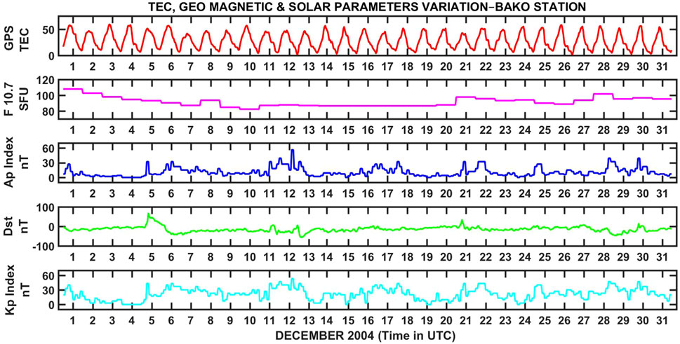
Figure 4. TEC, Geomagnetic and Solar parameters variations for December 2004.

Figure 5 shows a comparison of two different methods for measuring TEC over 8 days from 21 December 2004, to 28 December 2004. The two methods used are the ARMA and CoK models. The predicted TEC obtained from the two models are compared with the GPS TEC. Both ARMA and CoK models capture the general increasing trend in TEC values observed throughout the plotted period. The ARMA model closely follows the GPS TEC values until December 24th. The ARMA model shows a significant underestimation of TEC compared to the GPS TEC, with a difference of around 20 TECU. This discrepancy persists for December 27th. The ARMA model gradually recovers and starts aligning with the GPS TEC values again by December 28th. The CoK model generally tracks the GPS TEC values with some deviations throughout the period. The CoK model exhibits a smaller underestimation of TEC compared to the ARMA model, with a difference of around 5–10 TECU. Similar to the ARMA model, the CoK model gradually recovers and aligns with the GPS TEC values by December 28th. The observed discrepancies between the predicted and GPS TEC values, particularly around the day of the earthquake, could be indicative of ionospheric disturbances potentially triggered by the Sumatra earthquake. The larger underestimation by the ARMA model suggests it might be less sensitive to capturing these earthquake-induced TEC variations. The CoK model, with its smaller underestimation, might be slightly more responsive to the earthquake’s influence on the ionosphere.

Figure 5

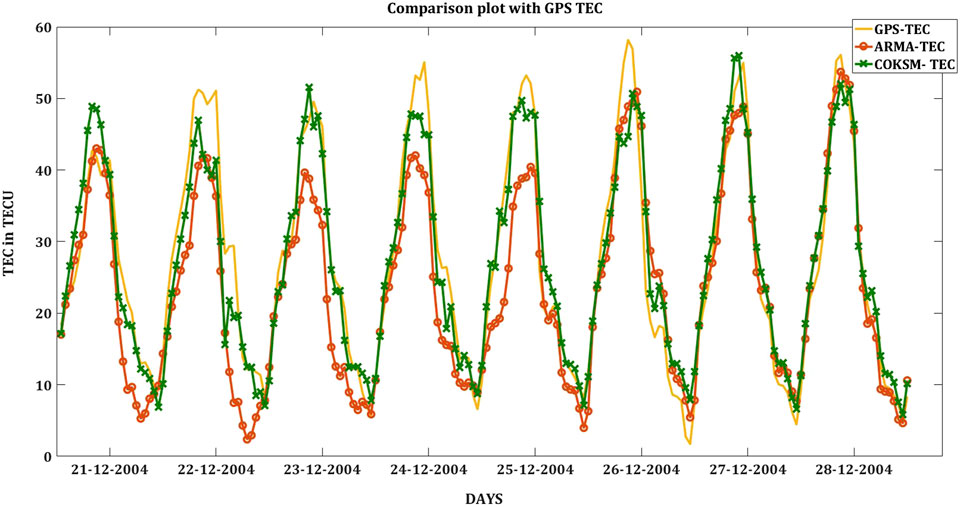
Figure 5. Comparison of GPS TEC and predicted TEC for the Sumatra Earthquake.

Figure 6 depicts the variations in Total Electron Content (TEC), a measure of ionization in the Earth’s ionosphere, over several dates in December 2004. All three plots (GPS TEC, ARMA TEC, and CoK TEC) show a gradual increase in TEC values (indicated by warmer colours like light green and parrot green, corresponding to 20–30 TECU) in the days leading up to December 26. This pre-earthquake ionospheric anomaly is consistent with the potential response of the ionosphere to the impending seismic event. Around December 26, the TEC values in all three plots exhibit fluctuations or sudden drops (represented by cooler colours like light blue and sky blue). This suggests ionospheric disturbances coinciding with the earthquake itself. Following the earthquake, the plots show varying patterns. The GPS TEC plot suggests a gradual decrease in TEC values (cooler colours), while the ARMA TEC and CoK TEC plots show a mix of increases, decreases, and stable TEC values. These variations suggest complex and potentially model-dependent ionospheric behaviour following the earthquake.

Figure 6

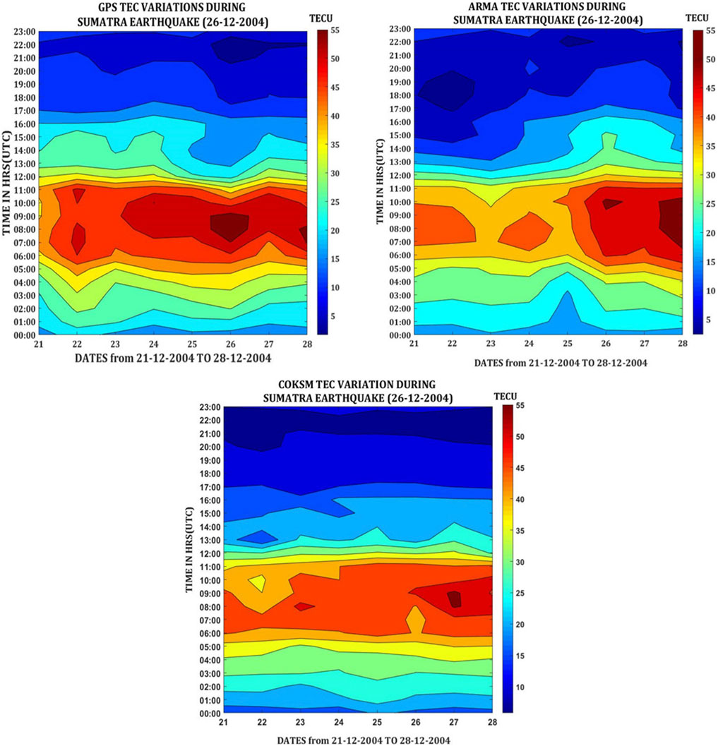
Figure 6. GPS TEC, ARMA, and CoK Predicted TEC variation contour during Sumatra Earthquake.

Figure 7A represents the comparison between ARMA-predicted TEC and GPS TEC as a linear regression scatter plot. The data points exhibit a relatively strong positive correlation, indicating a general alignment between ARMA-predicted TEC and GPS TEC values. However, there’s a moderate degree of spread, suggesting that the ARMA model does not perfectly capture all the nuances in the data. The slope of the best-fit line is slightly less than 1, indicating that the ARMA model tends to slightly underestimate TEC values, especially at higher magnitudes. The y-intercept is positive, signifying a potential small positive bias in the ARMA model predictions. The R-squared value of 0.844 indicates that the ARMA model explains about 84% of the variation in the GPS TEC data, suggesting a reasonably good fit. The linear regression analysis in Figure 7A reveals that the ARMA model demonstrates a good overall ability to predict the GPS TEC values. The high correlation and R-squared values support this.

Figure 7

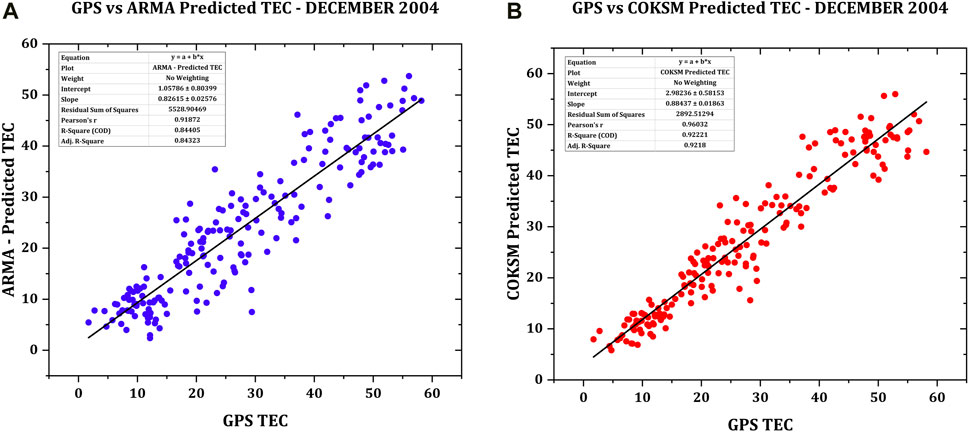
Figure 7. (A) Linear regression Analysis of ARMA TEC and GPS TEC. (B) Linear regression Analysis of CoK TEC and GPS TEC.

Figure 7B shows the comparison between predicted CoK TEC and GPS TEC as a linear regression scatter plot. The data points reveal a strong positive correlation between the CoK model predictions and the GPS TEC values. The slope of the line is very close to 1, indicating that the CoK model seems to capture the overall magnitude of TEC variations with less tendency for underestimation compared to the ARMA model as seen in Figure 7A. The y-intercept is a small positive value, suggesting a tiny positive bias in the CoK model. The R-squared value of 0.867 indicates that the CoK model explains approximately 87% of the variation in the GPS TEC data, suggesting a very good fit. The CoK model shows a slightly better fit to the GPS TEC data compared to the ARMA model, based on the higher R-squared value and reduced tendency for underestimation. Similar to the ARMA model, there’s a small positive bias observable in the y-intercept; however, it is very minor relative to the range of TEC values.

Table 1 provides an evaluation of the prediction method’s performance metrics, including RMSE, MAD, Relative error, and NRMSE for ARMA and CoK models. Employing statistical significance tests will help determine if the differences between the models are meaningful or likely due to random chance. In the pre-earthquake days, the CoK model exhibits lower RMSE values on most days, suggesting a slightly better fit to the GPS TEC data during this period. The MAD values are relatively close for both models, indicating similar-sized errors on average. On the earthquake day, the ARMA model shows notably lower error metrics on the day of the earthquake across all measures (RMSE, MAD, Relative Error and NRMSE). This could suggest increased accuracy for ARMA during a potentially disturbed period. After the earthquake day, RMSE/NRMSE: The CoK model regains its advantage with lower error values, indicating a potential return to a more regular ionospheric pattern for RNSE and NRMSE values. Similar to the pre-earthquake period, MAD values are comparable for both models, which suggests similar overall error magnitudes once the potential quake-induced disturbance subsides. The CoK model seems to perform slightly better in capturing general TEC trends in the days leading up to and immediately after the earthquake. The ARMA model’s outperformance on the specific day of the earthquake might be significant. This could potentially indicate it was more sensitive to earthquake-related ionospheric disturbances. Incorporating geomagnetic indices (Kp, Dst, Ap) during this period would help determine if increased solar activity or geomagnetic storms could contribute to the observed fluctuations and model differences. The CoK model demonstrates slightly better overall performance in the analyzed timeframe based on lower RMSE and NRMSE values for most days before and after the earthquake.

Table 1

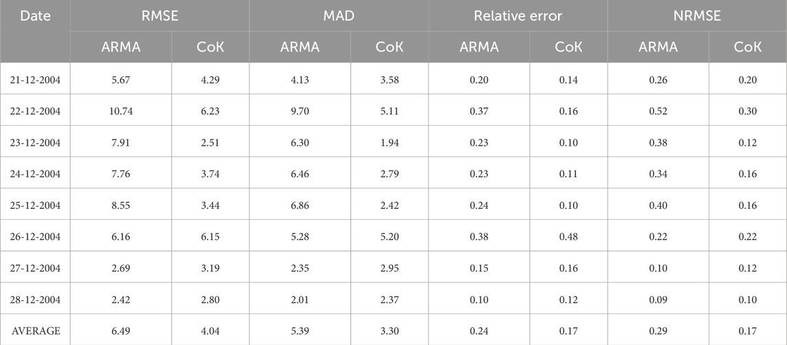
Table 1. Performance parameters for the Sumatra earthquake.

3.2 Prediction of TEC variations during Sulawesi earthquake

An earthquake with a magnitude of 6.6 hit 56.23 km southeast of Palu on Sulawesi Island in Indonesia with 6.5 magnitude. The focal depth of the earthquake was 20.11 Km. Figure 8 represents valuable insights into TEC, geomagnetic and solar parameter variations for December 2004. The x-axis represents time in days, ranging from August 1st to 31st, 2012. The y-axis shows TEC values in TECU, F10.7, Kp, Ap, and Dst. TEC exhibits a diurnal pattern, characterized by higher values during the daytime and lower values at night. The graph exhibits a general upward trend in TEC values throughout the month, with some fluctuations. The highest TEC value is around 77.05 TECU, while the lowest value is close to 1.37 TECU. There are a few notable dips in TEC throughout the month, particularly visible around August 12th. The Dst index is generally negative with a few dips below 50 nT, suggesting brief periods of moderately elevated geomagnetic activity. The Ap generally stays below 30, indicating relatively calm conditions, with a few spikes reaching above 30. The solar flux values display a gradual decline over the course of the month. Figure 9 represents a comparison of two different methods for measuring TEC over an eight-day period from 13 August 2012, 20 August 2012.

Figure 8

Figure 8. TEC, Geomagnetic and Solar parameters variations for August 2012.

Figure 9

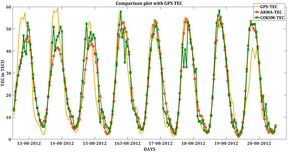
Figure 9. Comparison of GPS TEC and predicted TEC for the Sulawesi Earthquake.

Both ARMA and CoK models track the overall variations in the GPS TEC reasonably well. Their predictions capture the diurnal pattern in TEC behaviour throughout the plotted period. In the days leading up to the quake (August 13th – 17th), both models exhibit some minor deviations from the GPS TEC but largely follow the trend. The ARMA slight underestimation of TEC by the ARMA model compared to the GPS TEC on the earthquake day. The difference appears small, perhaps 5–10 TECU. The CoK model prediction also deviates, potentially even more so than the ARMA model, showing a slightly larger underestimation. Both models seem to realign with the GPS TEC relatively quickly in the days following the earthquake, although there may be some lingering discrepancies, especially with the CoK model. The observed deviations around the earthquake, especially by the CoK model, might suggest subtle ionospheric disturbances potentially associated with the Sulawesi earthquake.

Figure 10 depict variations in TEC, a measure of ionization in the Earth’s ionosphere, over several dates in August 2012. Examining all three figures, which showcase GPS TEC, ARMA TEC, and CoK TEC variations, alongside the provided colour scale revealing TECU values, reveals intriguing insights into the potential relationship between seismic activity and the Earth’s ionosphere. All three figures depict a gradual rise in TEC values (represented by warmer colors like light green and parrot green, corresponding to 20–30 TECU) in the days leading up to the 18 August 2012, earthquake. This pre-earthquake ionospheric anomaly, observed across all models, suggests a potential response of the ionosphere to the impending seismic event. Following the earthquake, the Figure 10 exhibit fluctuations in TEC values, with slightly varying patterns between the models, yet all indicating ionospheric disturbances after the seismic activity.

Figure 10

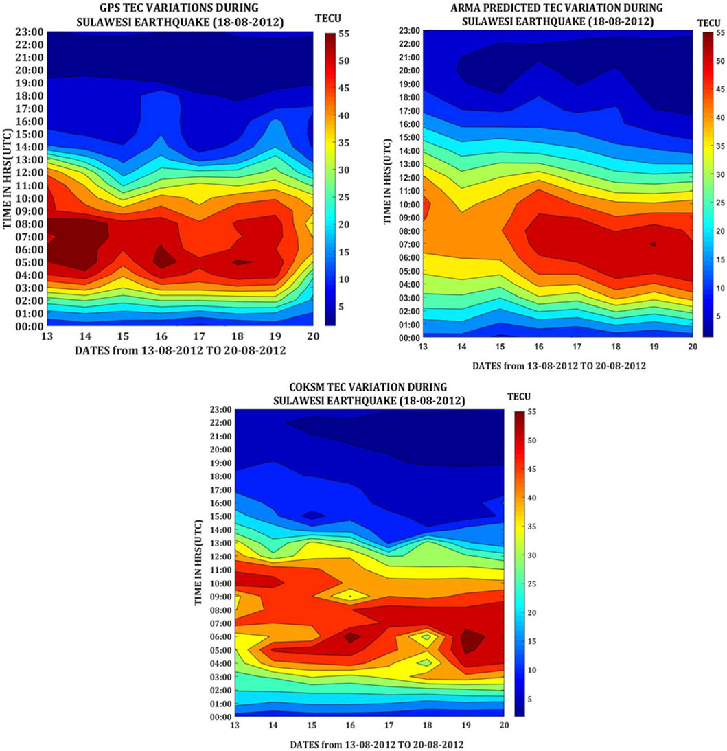
Figure 10. GPS TEC, ARMA, and CoK Predicted TEC variation contour plot during Sulawesi Earthquake.

Figure 11A represents the comparison between ARMA predicted TEC and GPS TEC as a linear regression scatter plot. The data points exhibit a relatively strong positive correlation, indicating a general alignment between ARMA predicted TEC and GPS TEC values. R-squared value of 0.8364 indicates that the ARMA model explains approximately 83.64% of the variance in the GPS TEC data. This suggests a moderately strong positive relationship between the predicted and GPS TEC values. R-squared value of 0.8364 is lower than the R-squared observed in Figure 6A, suggesting that the ARMA model explains a smaller percentage of the variation in the GPS TEC data for this specific period. The linear regression analysis in Figure 11A depicts a generally positive correlation between the ARMA model’s predictions and GPS TEC values.

Figure 11

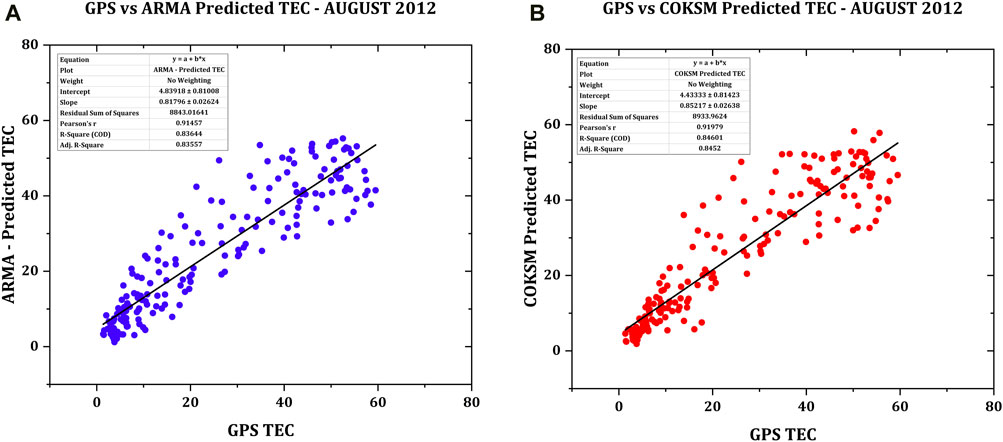
Figure 11. (A) Linear regression Analysis of ARMA TEC and GPS TEC. (B) Linear regression Analysis of CoK TEC and GPS TEC.

Figure 11B shows the comparison between ARMA predicted TEC and GPS TEC as a linear regression scatter plot. The data points reveal a positive correlation between CoK-predicted TEC and GPS TEC values. There’s less scatter compared to the ARMA model (Figure 11A), suggesting a stronger association between the predicted and actual TEC values. A higher R-squared value than Figure 11A indicates the CoK model explains a greater proportion of the variance in the GPS TEC data, suggesting a better fit compared to the ARMA model. The CoK model exhibits a stronger positive correlation between predicted and GPS TEC values, as evidenced by the tighter clustering of data points in the scatter plot compared to ARMA model. This suggests the CoK model performs better than the ARMA model in capturing the overall trend and variations in the GPS TEC data within this specific timeframe.

The performance evaluation parameters for the models during the Sulawesi EQ are given in Table 2. On the Pre-Earthquake days between 13-08-2012 to 17-08-2012, the CoK model exhibits lower errors across all metrics (RMSE, NRMSE, MAD, Relative Error), suggesting superior performance. The ARMA model has a noticeably lower RMSE/NRMSE, potentially indicating better handling of sudden fluctuations. The CoK model maintains its advantage in the MAD and Relative Error metrics. On post-earthquake days 19-08-2012 to 20-08-2012, the CoK generally regains its usual lower error values across the board. This pattern suggests that the earthquake might have temporarily disrupted the CoK model’s predictions, but it recovers quickly. The CoK model seems to perform slightly better in capturing general TEC trends in both the lead-up to and after the earthquake. This aligns with the concept that co-kriging techniques often excel in spatial modeling, which can translate to improved TEC predictions over time. The ARMA model’s outperformance on August 18th with lower RMSE/NRMSE is noteworthy. This could potentially indicate a greater sensitivity or responsiveness to ionospheric disturbances associated with seismic events. The ARMA model shows notably lower RMSE and NRMSE values on the specific day of the earthquake, potentially highlighting increased sensitivity to TEC changes during this period.

Table 2

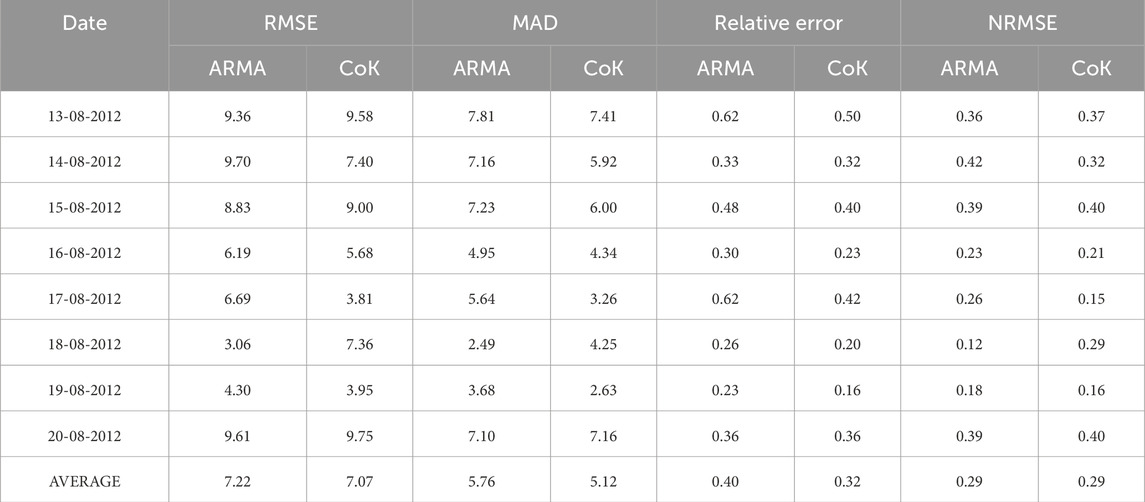
Table 2. Performance parameters for the Sulawesi earthquake.

4 Conclusion

The study investigated the feasibility of using Autoregressive Moving Average (ARMA) and CoKriging (CoK) models to forecast ionospheric Total Electron Content (TEC) variations preceding seismic events in Indonesia. Through analysis of two significant earthquakes–the December 2004 Sumatra earthquake and the August 2012 Sulawesi earthquake–along with associated TEC data, solar activity and geomagnetic indices, this research aimed to enhance our understanding of ionospheric dynamics and improve predictive capabilities for mitigating communication disruptions during seismic events. The analysis revealed distinct TEC variations preceding both earthquakes, with weak correlations to solar and geomagnetic activities but stronger associations with seismic-induced electric fields. The December 2004 Sumatra earthquake exhibited TEC variations 5 days prior to the event, while the August 2012 Sulawesi earthquake displayed variations 6 days before. The ARMA and CoK models were employed to predict TEC fluctuations, with evaluation metrics including Root Mean Square Error (RMSE), Mean Absolute Deviation (MAD), Relative Error, and Normalized RMSE (NRMSE) used to assess model accuracy. For the Sumatra earthquake, the ARMA model predicted a maximum TEC of 50.92 TECU with an RMSE of 6.15, while the CoK model predicted 50.68 TECU with an RMSE of 6.14. Similarly, for the Sulawesi earthquake, the ARMA model forecasted a maximum TEC of 54.43 TECU with an RMSE of 3.05, whereas the CoK model predicted 52.90 TECU with an RMSE of 7.35. Overall, both models captured the general trend in TEC variations preceding seismic events, but nuances emerged in their responses to seismic disturbances.

The ARMA model demonstrated heightened sensitivity to seismic disturbances, particularly evident on the day of the earthquake, indicating its potential for detecting short-term TEC anomalies associated with seismic events. Conversely, the CoK model exhibited more consistent performance across pre- and post-earthquake periods, suggesting its reliability in capturing long-term TEC variations. The comparison of evaluation metrics highlighted the strengths and limitations of each model, underscoring the importance of selecting appropriate modelling techniques based on specific application requirements. This research contributes to advancing our understanding of ionospheric behavior preceding seismic events and underscores the potential of predictive modelling in mitigating communication disruptions. The findings offer valuable insights into the complex interactions between seismic activity and ionospheric dynamics, informing the development of robust forecasting tools for enhancing navigation system resilience to seismic disturbances. Moving forward, further research endeavours may explore the integration of additional environmental factors, such as atmospheric conditions and Earth’s magnetic field variations, to refine predictive models and improve TEC forecasting accuracy. Additionally, investigations into the applicability of machine learning algorithms and ensemble modelling techniques could enhance the predictive capabilities of TEC forecasting systems, ultimately facilitating more effective mitigation strategies for communication disruptions during seismic events.

Data availability statement

Publicly available datasets were analyzed in this study. This data can be found here: The GPS TEC data is obtained from the IONOLAB website (http://www.ionolab.org/). The Geomagnetic and Solar indices were taken from the OMNIWEB DATA server (https://omniweb.gsfc.nasa.gov).

Author contributions

SK Conceptualization, Formal Analysis, Methodology, Writing–original draft. SM Validation, Writing–review and editing.

Funding

The author(s) declare that no financial support was received for the research, authorship, and/or publication of this article.

Conflict of interest

The authors declare that the research was conducted in the absence of any commercial or financial relationships that could be construed as a potential conflict of interest.

Publisher’s note

All claims expressed in this article are solely those of the authors and do not necessarily represent those of their affiliated organizations, or those of the publisher, the editors and the reviewers. Any product that may be evaluated in this article, or claim that may be made by its manufacturer, is not guaranteed or endorsed by the publisher.

References

Akyol, A. A., Arikan, O., and Arikan, F. (2020). A machine learning-based detection of earthquake precursors using ionospheric data. Radio Sci. 55, e2019RS006931. doi:10.1029/2019RS006931

CrossRef Full Text | Google Scholar

Cander, L. R. (1998). Artificial neural network applications in ionospheric studies. Ann. Geophys. 41 (5–6). doi:10.4401/ag-3817

CrossRef Full Text | Google Scholar

Draz, M. U., Shah, M., Jamjareegulgarn, P., Shahzad, R., Hasan, A. M., and Ghamry, N. A. (2023). Deep machine learning based possible atmospheric and ionospheric precursors of the 2021 Mw 7.1 Japan earthquake. Remote Sens. 15 (7), 1904. doi:10.3390/rs15071904

CrossRef Full Text | Google Scholar

Han, Y., Wang, L., Fu, W., Zhou, H., Li, T., and Chen, R. (2022). Machine learning-based short-term GPS TEC forecasting during high solar activity and magnetic storm periods. IEEE J. Sel. Top. Appl. Earth Observations Remote Sens. 15, 115–126. doi:10.1109/jstars.2021.3132049

CrossRef Full Text | Google Scholar

Huang, Z., and Yuan, H. (2014). Ionospheric single-station TEC short-term forecast using RBF neural network. Radio Sci. 49 (4), 283–292. doi:10.1002/2013rs005247

CrossRef Full Text | Google Scholar

Jiang, W., Ma, Y., Zhou, X., Li, Z., An, X., and Wang, K. (2017). Analysis of ionospheric vertical total electron content before the 1 April 2014 Mw 8.2 Chile earthquake. J. Seismol. 21 (6), 1599–1612. doi:10.1007/s10950-017-9684-y

CrossRef Full Text | Google Scholar

Joshi, S., Kannaujiya, S., and Joshi, U. (2023). Analysis of GNSS data for earthquake precursor studies using IONOLAB-TEC in the himalayan region. Quaternary 6 (2), 27. doi:10.3390/quat6020027

CrossRef Full Text | Google Scholar

Ke, F., Wang, Y., Wang, X., Qian, H., and Shi, C. (2015). Statistical analysis of seismo-ionospheric anomalies related to Ms > 5.0 earthquakes in China by GPS TEC. J. Seismol. 20 (1), 137–149. doi:10.1007/s10950-015-9516-x

CrossRef Full Text | Google Scholar

Koklu, K. (2023). Seismo ionospheric anomalies related to the Mw 7.5, Kepulauan Alor, Indonesia earthquake. Acta Geophys. 71 (6), 2633–2644. doi:10.1007/s11600-023-01165-7

CrossRef Full Text | Google Scholar

Liu, L., Morton, Y. J., and Liu, Y. (2022). ML prediction of global ionospheric TEC maps. Space Weather. 20 (9). doi:10.1029/2022sw003135

CrossRef Full Text | Google Scholar

Maheswaran, V. K., Baskaradas, J. A., Nagarajan, R., Anbazhagan, R., Subramanian, S., Devanaboyina, V. R., et al. (2024). Bi-LSTM based vertical total electron content prediction at low-latitude equatorial ionization anomaly region of South India. Adv. Space Res. 73 (7), 3782–3796. doi:10.1016/j.asr.2023.08.054

CrossRef Full Text | Google Scholar

Maltseva, O., and Mozhaeva, N. (2016). The use of the total electron content measured by navigation satellites to estimate ionospheric conditions. Int. J. Navigation Observation 2016, 1–15. doi:10.1155/2016/7016208

CrossRef Full Text | Google Scholar

Muhammad, A., Külahcı, F., and Birel, S. (2023). Investigating radon and TEC anomalies relative to earthquakes via AI models. J. Atmos. Solar-Terrestrial Phys. 245, 106037. doi:10.1016/j.jastp.2023.106037

CrossRef Full Text | Google Scholar

Mukesh, R., Dass, S. C., Vijay, M., Kiruthiga, S., Praveenkumar, M., and Prashanth, M. (2024). Analysis of TEC variations and prediction of TEC by RNN during Indonesian earthquakes occurred from 2004 to 2024 and comparison with IRI-2020 model. Adv. Space Res., doi:10.1016/j.asr.2024.07.055

CrossRef Full Text | Google Scholar

Mukesh, R., Karthikeyan, V., Soma, P., and Sindhu, P. (2020). Ordinary kriging - and cokriging - based surrogate model for ionospheric TEC prediction using NavIC/GPS data. Acta geophys. 68, 1529–1547. doi:10.1007/s11600-020-00473-6

CrossRef Full Text | Google Scholar

Nayak, K., Romero-Andrade, R., Sharma, G., Zavala, J. L. C., Urias, C. L., Trejo Soto, M. E., et al. (2023). A combined approach using b-value and ionospheric GPS-TEC for large earthquake precursor detection: a case study for the Colima earthquake of 7.7 Mw, Mexico. Acta Geod. Geophys. 58 (4), 515–538. doi:10.1007/s40328-023-00430-x

CrossRef Full Text | Google Scholar

Pulinets, S. (2004). Ionospheric precursors of earthquakes: recent advances in theory and practical applications. Terr. Atmos. Ocean. Sci. 15, 413–435. doi:10.3319/tao.2004.15.3.413(ep)

CrossRef Full Text | Google Scholar

Ratnam, D. V., Otsuka, Y., Sivavaraprasad, G., and Dabbakuti, J. R. K. K. (2019). Development of multivariate ionospheric TEC forecasting algorithm using linear time series model and ARMA over low-latitude GNSS station. Adv. Space Res. 63 (9), 2848–2856. doi:10.1016/j.asr.2018.03.024

CrossRef Full Text | Google Scholar

Reddybattula, K. D., Nelapudi, L. S., Moses, M., Devanaboyina, V. R., Ali, M. A., Jamjareegulgarn, P., et al. (2022). Ionospheric TEC forecasting over an Indian low latitude location using long short-term memory (LSTM) deep learning network. Universe 8 (11), 562. doi:10.3390/universe8110562

CrossRef Full Text | Google Scholar

Saqib, M., Şentürk, E., Sahu, S. A., and Adil, M. A. (2021). Ionospheric anomalies detection using autoregressive integrated moving average (ARIMA) model as an earthquake precursor. Acta Geophys. 69 (4), 1493–1507. doi:10.1007/s11600-021-00616-3

CrossRef Full Text | Google Scholar

Sezen, U., Arikan, F., Arikan, O., Ugurlu, O., and Sadeghimorad, A. (2013). Online, automatic, near-real time estimation of GPS-TEC: IONOLAB-TEC. Space weather. 11 (5), 297–305. doi:10.1002/swe.20054

CrossRef Full Text | Google Scholar

Sivavaraprasad, G., Deepika, V. S., SreenivasaRao, D., Ravi Kumar, M., and Sridhar, M. (2020). Performance evaluation of neural network TEC forecasting models over equatorial low-latitude Indian GNSS station. Geodesy Geodyn. 11 (3), 192–201. doi:10.1016/j.geog.2019.11.002

CrossRef Full Text | Google Scholar

Sur, D., Ray, S., and Paul, A. (2015). Role of neutral wind in the performance of artificial neural-network based TEC models at diverse longitudes in the low latitudes. J. Geophys. Res. Space Phys. 120 (3), 2316–2332. doi:10.1002/2014ja020594

CrossRef Full Text | Google Scholar

Tang, J., Li, Y., Yang, D., and Ding, M. (2022). An approach for predicting global ionospheric TEC using machine learning. Remote Sens. 14 (7), 1585. doi:10.3390/rs14071585

CrossRef Full Text | Google Scholar

Tebabal, A., Radicella, S. M., Nigussie, M., Damtie, B., Nava, B., and Yizengaw, E. (2018). Local TEC modelling and forecasting using neural networks. J. Atmos. Solar-Terrestrial Phys. 172, 143–151. doi:10.1016/j.jastp.2018.03.004

CrossRef Full Text | Google Scholar

Thomas, J. E., Ben, U. C., Ekanem, A. M., George, N. J., and Nathaniel, E. U. (2022). Seismo-ionospheric anomalies before M7.2 Haiti earthquake of August 14, 2021, from GPS-TEC. Acta Geophys. 70 (6), 2621–2627. doi:10.1007/s11600-022-00903-7

CrossRef Full Text | Google Scholar

Ulukavak, M., and Yalcinkaya, M. (2016). Precursor analysis of ionospheric GPS-TEC variations before the 2010M7.2 Baja California earthquake. Geomatics, Nat. Hazards Risk 8 (2), 295–308. doi:10.1080/19475705.2016.1208684

CrossRef Full Text | Google Scholar

Vankadara, R. K., Mosses, M., Siddiqui, M. I. H., Ansari, K., and Panda, S. K. (2023). Ionospheric total electron content forecasting at a low-latitude Indian location using a Bi-long short-term memory deep learning approach. IEEE Trans. Plasma Sci. 51 (11), 3373–3383. doi:10.1109/tps.2023.3325457

CrossRef Full Text | Google Scholar

Venkata Ratnam, D., and Sarma, A. D. (2012). Modeling of low-latitude ionosphere using GPS data with SHF model. IEEE Trans. Geoscience Remote Sens. 50 (3), 972–980. doi:10.1109/tgrs.2011.2163639

CrossRef Full Text | Google Scholar

Zhu, F., Su, F., and Lin, J. (2018). Statistical analysis of TEC anomalies prior to M6.0+ earthquakes during 2003–2014. Pure Appl. Geophys. 175, 3441–3450. doi:10.1007/s00024-018-1869-y

CrossRef Full Text | Google Scholar

Zhu, F., Yang, J., Qing, Y., and Li, X. (2023). Assessment and analysis of the global ionosphere maps over China based on CMONOC GNSS data. Front. Earth Sci. 11. doi:10.3389/feart.2023.1095754

CrossRef Full Text | Google Scholar