Measurement and calibration of non-linear shear terms in galaxy cluster fields

Introduction: Galaxy cluster lensing is a powerful tool for measuring the mass of galaxy clusters, but accurate shear measurement and calibration are critical to obtaining reliable results. This study focuses on the measurement and calibration of weak lensing shears to improve mass estimates in cluster lensing. To deal with the problem, we first developed an image simulation pipeline, jedisim, which utilizes galaxy images extracted from the Hubble Space Telescope (HST) Ultra Deep Field (UDF) and the Cosmic Assembly Near-infrared Deep Extragalactic Legacy Survey (CANDELS).

Methods: The simulations represent realistic galaxy distributions and morphologies as input sources. The foreground halo with a Navarro–Frenk–White (NFW) profile is constructed such that the lensing signals of background galaxies can be measured by the Vera C. Rubin Observatory’s Legacy Survey of Space and Time (LSST) Science Pipelines. By comparing the measured reduced shear $g^{\text{meas}}$ and the true reduced shear $g^{\text{true}}$, we observe non-linearity up to $g\lesssim 0.6$. We fit polynomials to the data with quadratic correction adequate to $g\lesssim 0.4$. Meanwhile, we conduct mass estimates using the pzmassfitter code on four different clusters.

Results: The mass estimate results are significantly improved after applying the shear calibration derived from the present work—from $4.954\pm 0.504\times 10^{14}{M}_{\odot }$ to $10.507\pm 0.498\times 10^{14}{M}_{\odot }$ after calibration for a simulated cluster with the mass of $10\times 10^{14}{M}_{\odot }$. In multiple cases of validation, the estimated results are all consistent with true cluster mass.

Discussion: This study yields the first relationship between reality and shape measurement of the LSST Science Pipelines and serves as the first step toward the overall goal of mass calibration in cluster lensing. By addressing the challenges in shear measurement and calibration, we aim to enhance the accuracy and reliability of mass estimates in galaxy cluster lensing studies.

1 Introduction

Although the $\mathrm{\Lambda }$CDM cosmological model shows phenomenological success, the nature of its two main components, dark matter and dark energy, is unknown. Therefore, physicists consider understanding these components as the major scientific driver in high-energy experiments and cosmological surveys. As an upcoming cosmological survey, the Vera C. Rubin Observatory Legacy Survey of Space and Time (LSST)¹ will provide an opportunity to understand the nature of dark matter and dark energy through its survey of the southern-hemisphere sky area (LSST Science Collaboration, 2009). Together with other space- and ground-based telescopes (e.g., the Nancy Grace Roman Space Telescope (Spergel et al., 2015) and the Euclid mission (Laureijs et al., 2011)), we will be able to acquire abundant high-resolution observational data in a wide sky area.

In LSST and another stage IV dark energy surveys, gravitational lensing plays a critical role, which describes the phenomenon that light from distant objects is bent by the gravitational field of intermediate-mass before arriving at the observers (Albrecht et al., 2006). Gravitational lensing provides a direct probe to determine the mass distribution in the Universe based solely on the gravitational effects of baryonic matter and dark matter. This probe is impartial and unbiased regarding the details of how the mass interacts (Van Waerbeke and Mellier, 2003).

Galaxy clusters, as the largest virialized structure, are formed in the relatively recent epoch of the cosmological age. Based on the observations and measurements from galaxy clusters, we can study the late-time evolution of the Universe and constrain cosmological parameters if the masses of the clusters are measured accurately. Among the analysis methods, weak gravitational lensing is an important and effective probe to estimate the masses (Joudaki et al., 2009). The most common measurement in weak lensing is the shape distortion (or shear) of galaxies, which describes the lensing effect. Therefore, to estimate the mass with high accuracy, we need to map the shapes of source galaxies to the mass of lenses. Before mapping, it is important to understand and restrict the systematics of shear measurements. To evaluate and improve the impacts of systematic bias, several data challenges, such as the Shear Testing Program (STEP) (Heymans et al., 2006; Massey et al., 2007) and the Gravitational Lensing Accuracy Testing (GREAT) (Bridle et al., 2009; 2010), have been conducted. In these data challenges, shear measurement biases are investigated and discussed in terms of the presence of realistic galaxy morphology, finite galaxy postage stamps, and galaxy types, among other factors, via different measurement methods (Mandelbaum et al., 2015). These data challenges have resulted in estimates for the calibration of shear measurements. These calibrations have been adopted for some recently completed and ongoing surveys (Heymans et al., 2006; Bridle et al., 2010; Mandelbaum et al., 2015). In general, the next-generation surveys are designed to measure the properties of dark energy at an order of magnitude of one percent accuracy, which can be considered the motivation of shear calibration (Bridle et al., 2009).

Taking the Hyper Suprime-Cam Subaru Strategic Program (HSC-SSP)² as an example, a set of simulations for shear calibration was analyzed by Mandelbaum et al. (2017), where realistic galaxy morphologies and nearby galaxies were taken into account with an effective source number density of 21.8 ${\mathrm{a}\mathrm{r}\mathrm{c}\mathrm{m}\mathrm{i}\mathrm{n}}^{-2}$. As an upcoming wide-area sky survey, LSST is capable of providing the largest and most uniform cluster sample with shape measurements to date. In the case of cluster weak lensing, the observational data will include weak lensing measurements for $\sim 40$ galaxies ${\mathrm{a}\mathrm{r}\mathrm{c}\mathrm{m}\mathrm{i}\mathrm{n}}^{-2}$ behind low redshift clusters (LSST Science Collaboration, 2009). Here, we evaluate the performance of the LSST Science Pipelines (LSP)³ in terms of both shear measurement and follow-up cluster mass reconstruction.

In this paper, we produce image simulations of cluster lensing. Real galaxy postage stamps are generated from Hubble Ultra Deep Field (HUDF) (Beckwith et al., 2006) and CANDELS (Grogin et al., 2011; Koekemoer et al., 2011) data release at the pixel scale of HST. These postage stamps are used to construct the background galaxies. A model foreground cluster is placed at a redshift between the observer and background galaxies. A ray-tracing algorithm is then adopted to apply the shear from the cluster to the background galaxies and simulate the lensed images. This simulation pipeline, known as jedisim⁴, is designed to output images under the observational conditions of LSST with the corresponding resolution.

The simulated images are processed and analyzed using the LSST Science Pipelines. Reduced shear is measured using the shapeHSM algorithm (Hirata and Seljak, 2003; Mandelbaum et al., 2017), and shear calibration biases can be derived by comparing the measured shear and true shear.

Before jedisim, there were already several well-developed image simulation pipelines for strong lensing effects, such as Pipeline for Images of Cosmological Strong (PICS) lensing, (Li et al., 2016) and SkyLens (Meneghetti et al., 2016; Plazas et al., 2019), as well as for weak lensing, such as GalSim (Rowe et al., 2015). Each of these simulation pipelines has its own advantages and is developed based on the necessary assumptions to optimize computational efficiency on a specific physics topic.

Our approach necessarily differs from the traditional simulation approach for weak lensing or strong lensing because massive galaxy clusters considerably distort galaxies located behind their central regions. Consequently, galaxies are not only more elliptical but also exhibit higher-order distortions (e.g., flexion), causing them to deform into rings or multiple images. One of our primary objectives is to investigate the impact of neglecting these higher-order distortions on cluster mass estimates, necessitating simulations that accurately reproduce the distortions. Because higher-order distortions can result in significant magnification of faint galaxies and noise features, we require that the template galaxies be free from noise. At the same time, we require that the galaxies have sufficient structures so that sub-image magnification can be handled correctly. Therefore, we developed our own image simulation pipeline.

Jedisim aims to simulate both strong and weak lensing effects in observations of a cluster field, where the galaxies retain the morphologies and properties of HUDF and CANDELS images. In addition, we apply the observational conditions of LSST to the simulation procedure and process the data with the entire analysis pipeline developed for LSST. Hence, the results are compatible with LSST and enlighten us to understand the output of the data analysis pipeline.

The remainder of this paper is organized as follows: in Section 2, we provide a brief review of the calculations and approximations in weak gravitational lensing, which are the fundamentals of the image simulation. The image simulation pipeline is described in Section 3. The methodology of the analysis pipeline is presented in Section 4. We summarize our results and conclusions in Sections 5, 6, respectively. Finally, we discuss systematics in Section 7 and present our conclusions in Section 8. Throughout this paper, we adopt the $\mathrm{\Lambda }$CDM cosmology and assume ${\mathrm{\Omega }}_m=0.315$, ${\mathrm{\Omega }}_{\lambda }=0.685$, and $H_0=67.8km{s}^{-1}Mp{c}^{-1}$ (Collaboration et al., 2020).

2 Gravitational lensing and the NFW profile

In this section, we provide a concise review of the calculations and approximations fundamental to weak gravitational lensing, which form the basis of our image simulation. Understanding these concepts is crucial for accurately modeling the lensing effects observed in galaxy clusters. We will discuss the equations and assumptions involved in weak lensing, highlighting their relevance to our simulation methodology.

2.1 Basic formalism of gravitational lensing

In the weak gravitational field limit, the gravitational lensing effect is described by the lens equation or ray-tracing equation denoted by Eq. 1 (Narayan and Bartelmann, 1996):

$\mathit{\beta }\left(\mathit{\theta }\right)=\mathit{\theta }-\mathit{\alpha }\left(\mathit{\theta }\right),(1)$

where $\mathit{\beta }$ is the true angular position, $\mathit{\theta }$ is the observed angular position, and $\mathit{\alpha }$ is the deflection angle. It is usually assumed that these two-component angles are small enough that the curvilinear nature of this coordinate system can be neglected.

Based on the thin lens approximation, where all the mass is in a single plane $P$ orthogonal to the direction of light and between the source and observer, we can treat space as Euclidean. In addition, because the deflection occurs in a small region compared to the path length, we can approximate the light path as a single deflection. Suppose that the projected mass density distribution on $P$ is given by $\mathrm{\Sigma }(\mathit{\xi })$, where $\mathit{\xi }$ is a vector in $P$.

Often, the mass distribution will not be planar but will be concentrated near the plane $P$. More precisely, let $z$ be a coordinate parallel to the path of the light. Then, the mass distribution is given by $\rho (\mathit{\xi },z)$ where $\rho =0$ for $\left|z\right|\ge \epsilon$, where $\epsilon$ is some distance which is smaller than the distance between the mass and the observer. This holds in almost all astronomical situations. In this case, $\mathrm{\Sigma }$ is given by integrating $\rho$ over the line-of-sight:

$\mathrm{\Sigma }\left(\mathit{\xi }\right)\equiv {\int }_{-\infty }^{\infty }\rho \left(\mathit{\xi },z\right),dz,(2)$

and $M(r)$, the mass enclosed within radius $r$, can be calculated by $\mathrm{\Sigma }(\mathit{\xi })$. In our simulations and observations, the distances involved are large enough that thin plane approximation is reasonable.

The angular diameter distances from the observer to the lens, observer to the source, and lens to the source are given by $D_{\ell }$, $D_s$, and $D_{\ell s}$, respectively. For a two-dimensional gravitational lensing potential $\psi$, the deflection angle can be written as $\mathit{\alpha }(\mathit{\theta })=\mathbf{\nabla }\psi$. The dimensionless surface mass density is represented as the convergence $\kappa$ denoted by Eq. 3:

$\kappa =\frac{1}{2}\left({\psi }_{11}+{\psi }_{22}\right)=\frac{\mathrm{\Sigma }}{{\mathrm{\Sigma }}_{\mathit{crit}}},(3)$

where ${\psi }_{ij}={\partial }^2\psi /\partial {\theta }_i\partial {\theta }_j$, and the critical surface mass density is given by Eq. 4

${\mathrm{\Sigma }}_{\mathit{crit}}=\frac{c_s^2}{4\pi G}\frac{D_s}{D_{\ell }{D}_{\ell s}},(4)$

where $c_s$ is the speed of light.

The shear $\gamma$ represents the tidal gravitational field of the lens and can be written as a complex notion $\gamma ={\gamma }_1+i{\gamma }_2$. These two components can be derived from the second derivatives of the lensing potential shown in Eqs 5, 6:

${\gamma }_1=\frac{1}{2}\left({\psi }_{11}-{\psi }_{22}\right),(5)$

${\gamma }_2={\psi }_{12}={\psi }_{21},(6)$

and the complex reduced shear is introduced as $g=\gamma /(1-\kappa )$. Without a measurement of the intrinsic size or magnification of a galaxy, we are only able to measure $g$ but not $\gamma$ (Schneider et al., 2000). Considering the weak lensing regime where $\kappa \ll 1$ and $\gamma \ll 1$, the image distortion due to the lensing cluster is usually much smaller than the intrinsic shapes of background sources. The convergence can be recovered by the shear $\gamma$ of background images through the inverse two-dimensional Laplacian to the potential $\psi$ (Fahlman et al., 1994; Kaiser et al., 1995; Fischer and Tyson, 1997). The distortion of the background image can be calculated by a Jacobian matrix denoted by Eq. 7 (Kaiser and Squires, 1993):

$\mathbb{A}=\left(1-\kappa \right)\left(\begin{array}{cc}\hfill 1-g_1\hfill & \hfill -g_2\hfill \\ \hfill -g_2\hfill & \hfill 1+g_1\hfill \end{array}\right).(7)$

Therefore, the distorted shape is a function of reduced shear $g$ rather than $\kappa$ or $\gamma$ separately. To describe the shapes of lensed galaxies, measuring their reduced shear along the tangential direction, $g_{\text{tan}}$, is more physically motivated than measuring $g_1$ and $g_2$, and $g_{\text{tan}}$ can be computed by the ellipticities of lensed sources (Schneider et al., 2000).

The measured ellipticity of a galaxy can be decomposed into two components: $e_1=e\cos (2\theta )$ along $x$ and $y$ axes and $e_2=e\sin (2\theta )$ along $y=\pm x$ directions, where $\theta$ is the position angle of the galaxy measured counter-clockwise from the $x$ axis. Furthermore, the shear of a galaxy can be quantified by its E-mode component, tangential ellipticity:

$e_{\text{tan}}=-\left(e_1\cos \left(2\varphi \right)+e_2\sin \left(2\varphi \right)\right),(8)$

where $\varphi$ is the azimuthal angle measured from the lens center and the factors of $\cos (2\varphi )$ and $\sin (2\varphi )$ project $e_1$ and $e_2$ to the tangential direction, respectively. The weak lensing effect on the background sources produces a curl-free stretching in the tangential direction to the line-of-sight. An image should have no systematic B-mode shear in background galaxies. If we omit the lens plane and assume the absence of intrinsic alignment of the background galaxies, the average tangential ellipticity should equal zero as a statistical result. Therefore, we can use $⟨e_{\text{tan}}⟩$ as an unbiased measurement of reduced shear. It is feasible to recover the convergence of a foreground galaxy cluster by calculating the non-zero average tangential ellipticity with a given sample of lensed background galaxies (Jarvis et al., 2003).

2.2 NFW profile

The Navarro–Frenk–White (NFW) profile is frequently used in mass distributions, as it is a good approximation to the average profile of clusters in N-body simulations and fits observations well. The profile has several dependent parameters, any two of which are sufficient (Navarro et al., 1996; 1997).

The NFW profile at redshift $z$ is defined as

$\rho \left(r\right)\equiv \frac{{\delta }_c{\rho }_c\left(z\right)}{\left(r/r_s\right){\left(1+r/r_s\right)}^2},(9)$

where ${\delta }_c$, ${\rho }_c$, and $r_s$ are parameters. The dimensionless characteristic density ${\delta }_c$ is given by

${\delta }_c\equiv \frac{200}{3}\frac{c^3}{\ln \left(1+c\right)-\frac{c}{1+c}},(10)$

where $c$ is the concentration parameter. ${\rho }_c$ is the critical density for closure of the Universe at redshift $z$ with units of mass density. It is given by Eq. 11

${\rho }_c\equiv \frac{3H^2\left(z\right)}{8\pi G},(11)$

where $H(z)$ is the Hubble parameter at redshift $z$. Furthermore, $r_s$ is a scale radius for the profile, with units of length and is given by $r_s\equiv \frac{r_{200}}{c}$, where $r_{200}$ is the radius within which the mean density of the halo is 200 times the critical density ${\rho }_c$. The mass enclosed by this radius is given by

$M_{200}\equiv M\left(r_{200}\right)=\frac{800\pi }{3}{\rho }_c{r}_{200}^3.(12)$

The NFW profile is given in three spatial dimensions; however, to use it with the thin lens approximation, we can compress it along the line-of-sight. Let $P$ be some plane through the origin and $z$ be the perpendicular direction through its origin. Let $R$ be the radial distance on the plane from the origin. Then, $\mathrm{\Sigma }(R)$, the surface mass density, is given by Eq. 2, except with $R$ instead of $\mathit{\xi }$ because of radial symmetry. To perform the integration, it is necessary to introduce the dimensionless distance variable $x\equiv R/r_s$. This integral is performed by Wright and Brainerd (2000), giving a complex but analytic expression:

$\begin{array}{cc}\hfill {\mathrm{\Sigma }}_{\text{NFW}}\left(x\right)& =2r_s{\delta }_c{\rho }_c\hfill \\ \hfill & \times \left\{\begin{array}{cc}\frac{1}{x^2-1}\left(1-\frac{2}{\sqrt{1-x^2}}\mathrm{a}\mathrm{r}\mathrm{c}\mathrm{t}\mathrm{a}\mathrm{n}\mathrm{h}\sqrt{\frac{1-x}{1+x}}\right)\hfill & 0\le x<1\hfill \\ \frac{1}{3}\hfill & x=1\hfill \\ \frac{1}{x^2-1}\left(1-\frac{2}{\sqrt{x^2-1}}\arctan \sqrt{\frac{x-1}{1+x}}\right)\hfill & 0\le x<1\hfill \end{array}\right.,\hfill \end{array}(13)$

where the constant $\frac{1}{3}$ is chosen to ensure continuity at $x=1$.

$M_{200}$ and $c$ are used to determine the deflection due to this profile since any two parameters are sufficient to describe the profile. Hence, ${\mathrm{\Sigma }}_{\text{NFW}}$ is integrated to calculate the enclosed mass. Since $R=r_{s}x$, the enclosed mass is is derived as Eqs 14, 15

$\begin{array}{cc}\hfill & M_{\text{NFW}}\left(x\right)=2\pi {\int }_0^x{\mathrm{\Sigma }}_{\text{NFW}}\left(x\right)RdR\hfill \\ \hfill & =2\pi r_s^2{\int }_0^x{\mathrm{\Sigma }}_{\text{NFW}}\left(x^{\prime }\right)x^{\prime }d{x}^{\prime }\hfill \\ \hfill & =2\pi r_s^{2}2r_s{\delta }_c{\rho }_c{\int }_0^{x}d{x}^{\prime }{x}^{\prime }\hfill \\ \hfill & \times \left\{\begin{array}{cc}\frac{1}{x^{\prime 2}-1}\left(1-\frac{2}{\sqrt{1-x^{\prime 2}}}\mathrm{a}\mathrm{r}\mathrm{c}\mathrm{t}\mathrm{a}\mathrm{n}\mathrm{h}\sqrt{\frac{1-x^{\prime }}{1+x^{\prime }}}\right)\hfill & 0\le x^{\prime }<1\hfill \\ \frac{1}{3}\hfill & x^{\prime }=1\hfill \\ \frac{1}{x^{\prime 2}-1}\left(1-\frac{2}{\sqrt{x^{\prime 2}-1}}\arctan \sqrt{\frac{x^{\prime }-1}{1+x^{\prime }}}\right)\hfill & x^{\prime }>1\hfill \end{array}\right.\hfill \\ \hfill & =4\pi r_s^3{\delta }_c{\rho }_c{\mathbb{X}}_{\mathit{NFW}}\hfill \\ \hfill & =\frac{M_{200}}{\ln \left(c+1\right)-\frac{c}{c+1}}{\mathbb{X}}_{\mathit{NFW}},\hfill \end{array}(14)$

where

$\begin{array}{c}\hfill {\mathbb{X}}_{\mathit{NFW}}=\ln \frac{x}{2}+\left\{\begin{array}{cc}\frac{2}{\sqrt{1-x^2}}\mathrm{a}\mathrm{r}\mathrm{c}\mathrm{t}\mathrm{a}\mathrm{n}\mathrm{h}\sqrt{\frac{1-x}{1+x}}\hfill & 0\le x<1\hfill \\ 1\hfill & x=1\hfill \\ \frac{2}{\sqrt{x^2-1}}\arctan \sqrt{\frac{x-1}{1+x}}\hfill & x>1\hfill \end{array}\right.\end{array},(15)$

with the first and third piecewise parts giving the entire expression, except at $x=1$. Due to the logarithm term, the enclosed mass diverges as $x\to \infty$, albeit quite slowly. Usually, the distribution is truncated to account for this, or $M_{200}=M_{\text{NFW}}(c)$ is used to describe the mass of clusters.

3 Simulations

The simulation pipeline, jedisim, was used to generate simulated cluster lensing images for Analysis of Realistic Cluster Lensing through Extensive Training Simulations (ARCLETS⁵). Simulated sheared galaxies and clusters are constructed to test for mass bias due to non-linearities in shear calibration. More details on implementation are included in Supplementary Appendix-1.

Any simulation is only as accurate as the model and parameters used to create it. Systemic biases are inevitably introduced by whatever differences exist between the simulation and actual galaxy clusters, as well as the errors in the galaxy properties of source galaxies. The best way to counteract this and reduce biases is to make the model and its parameters as physically accurate as possible. In practice, this is limited by the computational power available and the precision of the parameters used to calibrate the model. Judicious selection of what approximations and simplifications are used is required to make the model.

The jedisim pipeline models the effect of a foreground galaxy cluster on the shapes of background galaxies. Broadly, there are three main components of the simulation:

1. Making the field of supersampled background galaxies (Section 3.1);

2. Each galaxy image is then sub-pixel sampled, and the subpixels are separately ray-traced to model the process of distorting the light from the background galaxies in accordance with a specified mass distribution (Section 3.2);

3. The individual distorted galaxies are assembled into an image and then resampled onto an appropriate pixel scale, also accounting for the blurring and distortion due to the point spread function (PSF) and noise (Section 3.3).

The three steps are performed as independently as possible so that the model can be improved in a modular fashion. To enable strong lensing in practice, we have devised an efficient reverse-tracing technique that links the output sub-pixels to the input image, thereby allowing multiple imaging. Galaxies are simulated individually and combined into a single image at a late stage so that redshift-dependent effects can be included.

Furthermore, the simulation is generated across a wide sky area of $1200\times 1200$ ${\mathrm{a}\mathrm{r}\mathrm{c}\mathrm{s}\mathrm{e}\mathrm{c}}^2$, which is large enough that no lensing signal will be artificially removed by the image boundaries but small enough that the coordinates can be treated as flat. In the final step of the simulation, images are created with the observational conditions of LSST (see Section 3.3). To ensure that there are no pixelization effects when generating the galaxy light profiles, the first two steps are carried out at HST UDF resolution. The image is rescaled to LSST resolution in a subsequent step.

3.1 Background inputs

The background galaxy field is simulated one galaxy at a time. To create realistic lensed shapes, individual galaxies in the HDF/UDF and GOODS sky areas of CANDELS are identified by SExtractor. They are extracted and converted to $600\times 600$ ${\mathrm{p}\mathrm{i}\mathrm{x}\mathrm{e}\mathrm{l}}^2$ postage stamps. The stamps are applied with a mask thresholded at $5\sigma$ (per pixel), which is calculated based on the standard deviation in the sampled background sky area. This procedure aims to make sure that each postage stamp is noise-free and that the morphology feature of the galaxy is not artificially altered. In addition, distant sources and bright pixels that do not belong to the target galaxy are also masked out. Hence, each cleaned stamp has one isolated galaxy on a blank background, as shown in Figure 1.

Figure 1

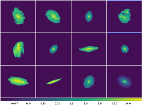
Figure 1. Sample $600\times 600$ pixel postage stamps cut out and cleaned from HST UDF with a pixel scale of 0.03 arcsec per pixel.

In this paper, we present simulation results only in r-band (552–691 nm) images for LSST. However, the database of jedisim contains postage stamps from HST WFPC2 (Wide Field and Planetary Camera 2) F450W, ACS (Advanced Camera for Surveys) F606W, and ACS F814W bands, which enable the potential of multi-band simulation (we discuss the simulation for the next step in Section 8). All the postage stamps are at an HST resolution of 0.03 arcsec per pixel. The sample repository contains 738 extracted galaxies, which can provide a fairly diverse set of galaxy shapes and orientations. More galaxy samples are planned to be included to increase the diversity in morphology, as discussed in Section 8.

The simulation aims to generate galaxies at the coadded depth with an r-band magnitude from 22 to 28.5, which is 1 mag deeper than the final coadded survey depth given by the LSST Science Book (LSST Science Collaboration, 2009). We calculate the AB magnitude for each galaxy postage stamp and convert them to magnitudes in LSST bands. When the sky is observed, a significant number of galaxies of high magnitude will be relatively faint. The noise level will then render them indistinguishable from the background. Because we generate simulations for both LSST 1-year and 10-year survey depths, they have different corresponding noise levels (see Section 3.3). So, we include the faint galaxies with a magnitude up to 28.5 to make sure the simulated sky has more realistic features. Based on the LSST Science Book (LSST Science Collaboration, 2009), $\sim 40$ galaxies per ${\mathrm{a}\mathrm{r}\mathrm{c}\mathrm{m}\mathrm{i}\mathrm{n}}^2$ behind the clusters are expected to be observed and measured. With this approximation of galaxy number density, $\sim 6000$ sources should be measured within a $\sim 150$ ${\mathrm{a}\mathrm{r}\mathrm{c}\mathrm{m}\mathrm{i}\mathrm{n}}^2$ simulation output, which is in good accordance with the results, as discussed in Section 6.

By using real galaxies as the materials of simulation, we retain the most morphological details in the galaxies. We have a finite dataset of the galaxy postage stamps with a sufficiently high signal-to-noise ratio from the HST field. Hence, it is necessary to increase the variety of samples in the simulation. Based on the originally extracted galaxy postage stamps, we create varied galaxies with realistic features. Each simulated galaxy is specified by six parameters detailed below:

• Magnitude: The magnitude of each galaxy is selected in the range of $22\le M\le 28.5$ with the distribution given by the power law denoted by Eq. 16:

$P\left(M+dM\right)\propto 10^{BM},(16)$

where $M$ is the r-band magnitude and $B=0.33\ln 10$ is an empirical constant (Benitez et al., 2004).

• Half-light radius: For each galaxy, the effective radius or half-light radius, $r_{50}$, is selected from the database of galaxy radii described by Kubo and Dell’Antonio (2008). This database is generated based on the galaxy magnitude-size distribution from HST UDF (Coe et al., 2006). Specifically, for statistical convenience, the database is binned by the integer part of the magnitude, and a list of radii is generated for each magnitude (the database is included in the source code of jedisim). Since each postage stamp is already assigned a magnitude, it has a corresponding bin, and an $r_{50}$ radius is chosen randomly from that bin. Then, the galaxy postage stamp is scaled to the new size using an interpolation routine.

• Image: A postage stamp image is chosen at random from those postage stamps whose $r_{50}$ value is larger than $r_{50}$ assigned to the galaxy. Hence, the images are always sized down to avoid interpolation errors.

• Redshift: The database of galaxy redshift from the zCOSMOS redshift survey is used and binned by magnitude (Iovino et al., 2010). For each galaxy, a redshift is selected from the corresponding magnitude bin. Alternatively, a single redshift (i.e., $z=1.5$) can be chosen for all galaxies. This parameter can be controlled in the configuration file of jedisim. When $z=1.5$ is selected for the source galaxies, their luminosities and pixels are rescaled according to their intrinsic redshifts.

• Position: The center of the postage stamp is selected as a pair of uniformly distributed floating points (for $x$ and $y$ positions in pixel). The range of position is restricted to ensure that the entire galaxy postage stamp lies completely within the simulated image.

• Orientation: Each galaxy is randomly oriented by choosing an angle uniformly from the range $[\mathrm{0,2}\pi )$. The orientation of galaxies has at least three degrees of freedom, but since we are dealing with two-dimensional projections of galaxies, we can only make the orientation random in one degree of freedom, with some additional variability coming from the diverse orientations of the postage stamps.

Once these parameters are chosen for each galaxy, an image is made that satisfies those parameters. The postage stamp is rotated at the assigned angle, scaled down to the correct $r_{50}$ radius (using bilinear interpolation), and its flux is adjusted to the correct magnitude. The galaxy is then appropriately cropped so that the image consists of the smallest rectangle that contains all non-zero pixels of the galaxy. Each transformed postage stamp galaxy is saved as a FITS image, along with the six parameters that characterize it.

Therefore, we have all the information on the background simulation image: a catalog of galaxies whose sizes, magnitudes, orientations, positions, and (optionally) redshifts are distributed in accordance with observations.

3.2 Lensing model

The next step in the simulation is to emulate the effects of gravitational lensing caused by a galaxy cluster. As mentioned in Section 2.1, the lens equation can be written as Eq. 17

$\mathit{\beta }\left(\mathit{\theta }\right)=\mathit{\theta }-\mathit{\alpha }\left(\mathit{\theta }\right)=\mathit{\theta }-\frac{D_{\ell s}}{D_s}\widehat{\mathit{\alpha }}\left(\mathit{\theta }\right),(17)$

where the deflection term $\widehat{\mathit{\alpha }}$ is a vector quantity in a radially symmetric mass distribution as in Eq. 18.

$\widehat{\mathit{\alpha }}\left(\mathit{\theta }\right)=\alpha \left(r\right)\widehat{\mathit{r}},(18)$

where $\alpha (r)$ is the radial deflection which depends on the mass distribution, $r$ is the distance from the center of the mass distribution to $\mathit{\theta }$, and $\widehat{\mathit{r}}$ is the unit vector from the center of the mass distribution to $\mathit{\theta }$. Both $r$ and $\alpha (r)$ have units of pixels.

We implement the density distribution profile as a separate module in the code, which enables jedisim to simulate different types of galaxy clusters. In this work, we use the NFW profile (Navarro et al., 1996; 1997) to generate the images, as it provides a well-established model for the mass distribution of galaxy clusters. Additionally, the specific cluster field we are studying is not significantly affected by the potential issues associated with the central density divergence of the NFW profile.

For an NFW profile cluster, given Eqs 9, 10, 12, its virial mass can be written in terms of the concentration $c$shown in Eq. 19:

$M_{200}=4\pi {\rho }_c{\delta }_c{r}_s^3\left[\ln \left(1+c\right)-\frac{c}{1+c}\right].(19)$

Then, the density is expressed as $\rho (r;M_{200},c)$. The deflection in pixels by the NFW profile is given by Eq. 20

$\frac{\alpha \left(r;M_{200},c\right)}{r}=\frac{4G{M}_{200}{\delta }_c^{\prime }}{9\times 10^5{D}_{\ell }r}\times {\mathbb{X}}_{\mathit{NFW}},(20)$

where $r$ is the radius in pixels, $D_{\ell }$ is the angular diameter distance of the cluster for a given cosmology, and ${\delta }_c^{\prime }$ is a modification of the density parameter, which is given by Eq. 21

${\delta }_c^{\prime }=\frac{1}{\ln \left(1+c\right)-\frac{c}{1+c}},(21)$

and $x$, as defined in Eq. 13, is calculated by Eq. 22

$x=\frac{Sc{D}_{\ell }}{10.0}{\left(\frac{G}{H_0^2}\right)}^{-1/3}r,(22)$

where $H_0$ is the Hubble constant at the present time and $S$ is the conversion factor between pixels and radians given by Eq. 23

$S=\frac{\pi }{180\left(\text{degree}\right)}\frac{3600\left(\text{arcsec/degree}\right)}{\text{resolution}\left(\text{arcsec/pixel}\right)}.(23)$

An arbitrary number of lenses can be present simultaneously, whose center positions, redshifts, and profile parameters are all specified by a configuration file. In this work, we use a single symmetric lens to produce simulations. In the future, however, we plan to enable the potential probability to simulate substructures of clusters or the light cone of multiple lensing planes. The lenses can be distributed at any redshift, as described in the configuration file. To simplify the mass reconstruction process at this first stage, all lenses share the same redshift in the current simulation. The deflection then becomes the superposition of the deflections from each of the lenses: if there are $N$ lenses with deflection functions ${\alpha }_i$ for $i=1,\dots ,N$, then the deflection term becomes Eq. 24

$\widehat{\mathit{\alpha }}\left(\mathit{\theta }\right)={\displaystyle \sum _{i=1}^N}{\alpha }_i\left(r_i\right){\widehat{\mathit{r}}}_i,(24)$

where $r_i$ is the distance from the center of the $i$^th mass distribution to $\mathit{\theta }$ and ${\widehat{\mathit{r}}}_i$ is the corresponding unit vector.

The lensed image is calculated by applying Equation $(17)$ to the subsampled background image produced in Section 3.1. This is done as follows. For now, assume that all background galaxies lie at a single redshift. Then, we can consider the Universe as consisting of three parallel planes: the source plane, where the background galaxies lie; the lens plane, where the mass distribution lies; and the observation plane, which is near Earth but above the atmosphere.

Any light traveling from the source plane to the observation plane will pass through the lens plane and be deflected, forming a distorted image of the source plane on the observation plane. A straightforward way to determine what this distorted image will be is to trace the path of individual photons from the source image to the observation image. Unfortunately, this is non-deterministic because of the phenomenon of multiple images and is thus extremely inefficient. However, it is possible to go backward. Concretely, let $I$ and $J$ be the scalar-valued intensity function on the source and observation planes, respectively, and let $\widehat{\mathit{\alpha }}$ be the vector-valued deflection function on the lens plane. Then, with $\mathit{\theta }=(x,y)$,

$J\left(x,y\right)=I\left(\mathit{\beta }\left(x,y\right)\right)=I\left(\left(x,y\right)-\frac{D_{\ell s}}{D_s}\widehat{\mathit{\alpha }}\left(x,y\right)\right).(25)$

This Eq. 25 contains the assumption from above that all background objects have a single redshift. In a more realistic case where there are background galaxies at multiple redshifts, there is a separate source plane for each redshift, and a corresponding observation plane can be calculated for each one. Hence, the total observation intensity is the sum of all these planes.

3.3 PSF and noise

To emulate the actual atmospheric and telescopic effects in observation, we make a non-varying point spread function using PhoSim⁶ with a $\delta$-function input (Peterson et al., 2015). The distorted, denoised galaxy postage stamps are assembled into the final sky area and then convolved with this PSF kernel.

By modifying the parameters of PhoSim, the PSF kernel is generated at the HST resolution with the observational conditions of LSST. The resulting PSF is normalized to a total intensity of unity, as illustrated in Figure 2.

Figure 2

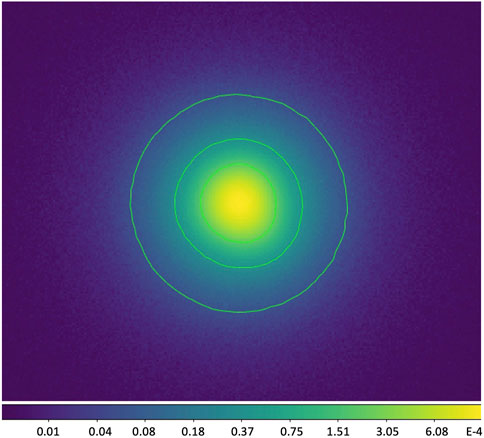
Figure 2. Normalized PSF convolution kernel at the HST resolution, generated by PhoSim and displayed in the log-scale.

To ensure that the final simulation image at the LSST resolution has a smooth and realistic PSF, the PSF image we generate at the HST resolution has a size of $1024\times 1024$ pixels, so it is computationally impractical to convolve straight from the double-sum two-dimensional discrete convolution. At a small loss of precision, it is more efficient to utilize the convolution theorem. A strip with a width of 1024 pixels is added to each image so that no information is lost. Using the FFTW3 library, each image is Fourier transformed, multiplied with the transform of the PSF, and transformed back. The image is then trimmed by 1024 pixels to recover the original dimension. Because this image is still at HST resolution (0.03 arcsec per pixel), it is resampled to the LSST resolution of 0.2 arcsec per pixel by block averaging.

In this process of generating PSF, the size of seeing is set at 0.7 arcsec based on the observational condition of LSST (LSST Science Collaboration, 2009). The PSF ellipticity is $e_1=-0.0020$ and $e_2=-0.0050$ (measured by SExtractor). In a later step, we simulate stars based on this PSF kernel.

In addition, we add Poisson noise to each pixel. To acquire an empirical estimate of the noise level, we measure the variance of background noise from random samples of the sky area in the Dark Energy Camera (DECam) r-band images of Abell 3128 with 1-year depth (McCleary et al., 2015). By calculating the average value, we use this variance $\lambda$ as the parameter in our simulation images with 1-year depth and downscale the parameter for images with 10-year depth accordingly. The size of the sampled sky area is varied according to the local distribution of detectable objects to make sure that no distinguishable galaxy or star is included and is not significantly contaminated by undetected objects.

For validation, the simulations have an average number density of $\sim 39.8$ ${\mathrm{a}\mathrm{r}\mathrm{c}\mathrm{m}\mathrm{i}\mathrm{n}}^{-2}$ for detectable background sources in 10-year coadded depth as measured by the LSST Science Pipelines, which is consistent with our expected value for LSST. More measurement parameters are described in Section 4.3.

3.4 Cluster simulations

On the basis of NFW-profile galaxy clusters, as discussed in Section 3.2, we generate four groups of cluster simulations with a size of $12.2\times 12.2$ ${\mathrm{a}\mathrm{r}\mathrm{c}\mathrm{m}\mathrm{i}\mathrm{n}}^2$ ($24576\times 24576$ pixels at the HST resolution). The foreground cluster in each group has a virial mass of $\mathrm{5,10,15,20}\times 10^{14}{M}_{\odot }$, respectively. The concentration of all clusters is set to 4.0.

The clusters are placed at $z=0.3$ with only dark matter halo such that no extra bias is introduced due to foreground–background blending. The background galaxies are sampled from our HST ACS F606W postage stamp database. The background source plane is set at $z=1.5$ with 30,000 galaxies as raw input, whose r-band magnitudes range from 22 to 28. The galaxy number count is extrapolated from ACS observations by Benitez et al. (2004), where 799,663 galaxies per square degree are detected in the F606W filter with a magnitude up to 27.29.

After lensing, the output is down-scaled from HST resolution to LSST resolution by interpolation. All images are convolved with the LSST PSF kernel and have background noise added, as introduced in Section 3.3. For each simulation, images for both 1-year and 10-year survey depths are generated. An example is shown in Figure 3 with cluster virial mass $M_{200}=20\times 10^{14}{M}_{\odot }$.

Figure 3

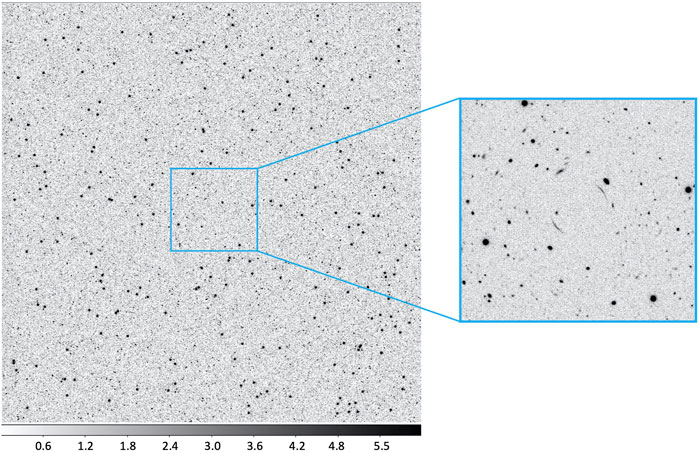
Figure 3. One cluster simulation with $M_{200}=20\times 10^{14}{M}_{\odot }$ in 10-year depth. Left: the full $12.2^{\prime }\times 12.2^{\prime }$ field of view of the cluster $(z=0.3)$ and background galaxies $(z=1.5)$ at an LSST resolution ($0.2^{″}/$pixel). Right: zoomed-in view of the central $2.3^{\prime }\times 2.3^{\prime }$ area, which shows strong lensing arcs. The image is displayed in the z-scale.

To diminish the intrinsic shape bias of the background galaxy sample and increase computational efficiency, we generate variant simulations where each selected background galaxy is rotated by 90° before lensing and assemble a separate simulated image with other parameters unchanged.

3.5 Grid simulations

The cluster simulations described in Section 3.4 are capable of simulating lensing distortion from weak to strong lensing regimes. However, similar to realistic cluster fields, there are blendings between background galaxies in these simulations. Hence, we also generate simulated images in a grid layout in addition to the cluster simulations to study the mapping between measured tangential ellipticity and true reduced shear.

In the grid-layout simulations, every single galaxy is assigned a known true reduced shear $g^{\text{true}}$. To achieve this, each background galaxy is generated via the same ray-tracing simulation pipeline, as introduced in Section 3.4. Then, postage stamps of the lensed galaxies are cut out and assembled into a grid layout. The range of $g^{\text{true}}$ is designed from 0.02 to 0.60, which covers from weak lensing to strong lensing regime. After lensing, the distorted galaxies are rescaled to the LSST resolution and arranged in a grid layout with the size of $1900\times 1900$ pixels. Similarly, the images are convolved with the LSST PSF kernel. For a higher signal-to-noise ratio in detection, we only add sky noise at the level of the 10-year survey depth. An example is illustrated in Figure 4.

Figure 4

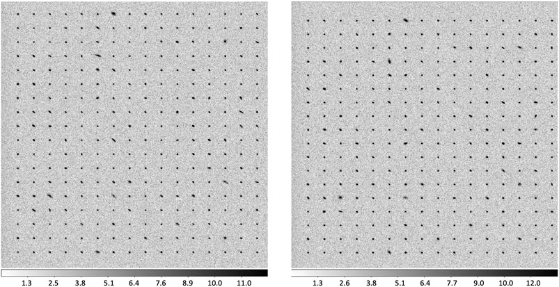
Figure 4. Grid simulation generated with $g=0.4$ in 10-year depth. Left: the full $\mathrm{1,900}\times 1900$ pixel image at an LSST resolution ($0.2^{″}/$pixel). Right: the corresponding parallel image with each galaxy rotated by $90°$ before lensing. In both images, the individual galaxies are placed at an azimuthal angle of $60°$ relative to the cluster center. Because the given reduced shear is relatively strong, it is noticeable that the lensed galaxies share the same trend of distortion. Images are displayed in the z-scale.

As discussed in Section 3.4, a parallel set of grid simulations is produced with each galaxy postage stamp rotated by $90°$ before lensing to suppress intrinsic shape noise. Furthermore, to reduce bias in the intrinsic orientation of the galaxy sample, postage stamps are placed at different azimuthal angles (i.e., $0°$, $60°$, $120°$, $180°$, $240°$, and $300°$) with respect to the cluster center. A total of 410 grid simulations in the F606W band are generated, including 60 sets of simulations per azimuthal angle plus 50 sets for null tests. Each simulated image contains 300 to 1,000 individual galaxies, depending on their actual sizes and separations. To make it possible to be processed by the analysis pipeline, normalized PSF stars are added in the gaps between separate galaxies, such that they can be detected and measured by the LSST Science Pipelines. We will demonstrate in the next section how to measure the calibration biases from the simulations.

4 Methods of analysis

To analyze the simulations, we process the images using the LSST Science Pipelines with appropriate configurations. By processing the images through LSP, we obtain shape measurement outputs, which enable us to conduct a series of analyses. These analyses allow us to estimate the reduced shear and derive the mass of the galaxy clusters.

4.1 LSST Science Pipelines

The LSST Science Pipelines are developed to satisfy the rapid cadence and scale of the LSST observing program for image and data processing. A prototype of the LSST Science Pipelines is also used as the fundamental codebase of the HSC Pipeline to reduce HSC Subaru Strategic Program (SSP) data. Details about the software architecture, algorithms, and processing tasks are described by Jurić et al. (2015) and Bosch et al. (2017).

In the analysis of our simulations, we use an LSP installation of the v17.0 release, together with the obs_file⁷ package as an interface to ingest and process the simulation images. The obs_file package was developed explicitly for the work presented in this paper. Because we have perfect knowledge of the PSF kernel and background noise, several tasks in the LSST Science Pipelines can be simplified. Specifically, the CCD processing step consists of instrumental signal removal (ISR), source detection, PSF measurement, aperture correction, deblending, and source measurement.

In the context of the LSST Science Pipelines, a sky area with all pixels above the detection threshold is defined as a footprint. One footprint can include one or multiple peaks. Although foreground–background blending situations are eliminated in our cluster simulations, blending instances between background galaxies still occur. In this case, a footprint with multiple peaks is considered a “parent” source, while the deblended sources and single-peak footprints are “children” sources.

The images are generated to simulate the coadded exposures in 1-year and 10-year depths, so they do not require joint calibration through the pipeline. Therefore, the tasks invoked in this pipeline are equivalent to single-frame processing subtasks, followed by coaddition detection and measurement. In the simulation images, each FITS file only includes the image extension but not the mask or variance extensions. Hence, the primary parameter as an input is the estimated background noise given in analog-to-digital unit (ADU), which is an estimate of the background field required by ISR such that some isolated noise pixels are not detected as cosmic rays. According to the original average noise used to generate the simulations and the measured background variance in the simulated images, we set this input sky noise level as $\mathtt{i}\mathtt{s}\mathtt{r}.\mathtt{n}\mathtt{o}\mathtt{i}\mathtt{s}\mathtt{e}=5.0$ for 10-year depth and $\mathtt{i}\mathtt{s}\mathtt{r}.\mathtt{n}\mathtt{o}\mathtt{i}\mathtt{s}\mathtt{e}=15.0$ for 1-year depth. Since these noise values are used as initial estimates that the pipeline can update afterward, there is a slight tolerance in them, but the estimates still should be made reasonably. Theoretically, there is no cosmic ray added when generating the simulated images. As a result, the pipeline identifies 0 cosmic rays in CCD processing as expected.

4.2 Astrometry and PSF modeling

The simulations are originally produced with no World Coordinate System (WCS) coordinates because, with the obs_file package, images are processed and measured at pixel level without R.A./Dec. information. Accordingly, the measured x/y positions and second-order moments are in pixel coordinates.

However, in the later steps of mass estimation, the pipeline requires WCS information in R.A. and Dec. Given the relatively small dimensions of the simulated images, we add flat WCS coordinates to the image headers with a pixel scale of $0.2^{″}$.

In addition, the LSST Science Pipelines require a PSF model for shape measurement. We add 200 PSF stars randomly into the $12.2^{\prime }\times 12.2^{\prime }$ field of view of cluster simulations. The stars are generated, as described in Section 3.3. For the PSF measurement, a maximum-likelihood detection algorithm is adopted with a $50\sigma$ threshold and $1^{″}$ full width at half maximum (FWHM) Gaussian as the smoothing filter (Bosch et al., 2017). Two iterations of the PSF star selector are implemented with updated median background values to determine the sources used as PSF. Consequently, only enough bright stars are selected for PSF modeling and fed into PSFEx based on analysis of the measured sizes (Bertin, 2013). To confirm the accuracy of the PSF measurement, we compare the positions and the size of the detected PSF stars with their ground truth inputs.

4.3 Image processing

Once the data are ingested appropriately, each CCD is processed independently, producing a calibrated image and its corresponding source catalog. A long series of semi-iterative subtasks are included in this task. To process the simulations, we invoke ISR, source detection, aperture correction, background subtraction, deblending, and source measurement. Due to a relatively simple instrument signature, no brighter-fatter or crosstalk corrections are employed in ISR. A $5\sigma$ threshold is applied for detected positive sources, which are recorded as footprints.

The deblender algorithm is applied if a footprint contains more than one peak. The flux of the footprint is apportioned such that one “child” image is created for each peak as a distinct source. Both “parent” and “children” sources are measured and stored: each “parent” together with its “children” sources is assigned a unique parent ID, while the number of “children” sources in each deblended “parent” source is recorded as deblend_nChild. Some important parameters and features of the LSST Science Pipelines are listed in Table 1.

Table 1

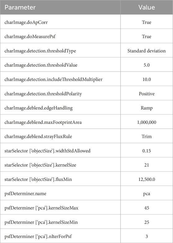
Table 1. Parameters in process CCD.

The primary data outputs of CCD processing are calexp (calibrated exposures) and src (source catalogs). The calexp files are the output FITS images with multi-extensions after CCD processing. They contain calibration and correction information, as well as objects for PSF modeling. The src files are in the format of the FITS table, where each source is stored as one entry. The columns in the catalogs represent characterizations and measurements of the objects. The catalogs also contain an array of flags, in which a flag of calib_psfCandidate indicates whether the source is selected as a PSF candidate. To obtain a clean catalog that has only distinct galaxy sources, we apply a filter with criteria $\mathtt{d}\mathtt{e}\mathtt{b}\mathtt{l}\mathtt{e}\mathtt{n}\mathtt{d}\text{\_}\mathtt{n}\mathtt{C}\mathtt{h}\mathtt{i}\mathtt{l}\mathtt{d}=0$ and $\mathtt{c}\mathtt{a}\mathtt{l}\mathtt{i}\mathtt{b}\text{\_}\mathtt{p}\mathtt{s}\mathtt{f}\mathtt{C}\mathtt{a}\mathtt{n}\mathtt{d}\mathtt{i}\mathtt{d}\mathtt{a}\mathtt{t}\mathtt{e}=\mathtt{F}\mathtt{a}\mathtt{l}\mathtt{s}\mathtt{e}$ on the src catalogs.

4.4 Shape measurements

This version of the LSST Science Pipelines employs the shapeHSM algorithm (HsmMoments) to measure the adaptive Gaussian moments, where the Gaussian elliptical weight functions are iteratively calculated and matched to the measured moments (Bosch et al., 2017). The adaptive moments $\mathbb{M}$ are calculated with the least-squares deviation from the image pixels. Hence, the ellipticity tensor $(e_{+},e_{\times })$ can be determined by the second moments as shown in Eqs 26–28.

$e_{+}=\frac{M_{xx}-M_{yy}}{T},(26)$

$e_{\times }=\frac{2M_{xy}}{T},(27)$

where $T$ is the trace,

$T=\left(M_{xx}+M_{yy}\right),(28)$

and ellipticity $e$ used in this paper is the same as $\chi$ in Schneider (2006).

The HsmMoments output is implemented from the HSM measurement in GalSim (Rowe et al., 2015). In this algorithm, the PSF-corrected ellipticities are estimated in addition to adaptive moments so that the PSF-corrected shears can be calculated as output. Explicitly, ext_shapeHSM_HsmShapeRegauss_e1 and ext_shapeHSM_HsmShapeRegauss_e2 are the results using the re-Gaussianization method, as described in Hirata and Seljak (2003).

The HSM measurement has the following advantages:

• Robustness and validation: The HSM measurement has been rigorously tested and validated across various datasets and surveys (Miller et al., 2013; Mandelbaum et al., 2018). Its performance and reliability are well-documented, making it a dependable choice for shear measurement in our study.

• Simplicity and efficiency: Compared to forward modeling and machine learning methods, re-Gaussianization is computationally less intensive and easier to implement, allowing for efficient processing of large datasets.

• Baseline comparability: Using a well-established method like HSM measurement provides a baseline for comparison with other studies in the field, facilitating the validation and interpretation of our results within the broader context of weak lensing research.

We realize and consider other shape measurement methods. Forward modeling techniques involve generating model images of galaxies and fitting these models to the observed data to extract shear estimates. This method is advantageous as it allows for the direct incorporation of complex PSF models and galaxy morphologies, potentially leading to more accurate shear measurements (Bernstein and Jarvis, 2002a; Miller et al., 2007; Voigt and Bridle, 2010). Machine learning approaches, such as convolutional neural networks (CNNs), have been increasingly explored for shear measurement. These methods can learn complex, non-linear relationships between observed galaxy images and shear, potentially outperforming traditional methods, especially in cases with significant noise and PSF distortions (Ribli et al., 2019; Tewes et al., 2019; Zhang et al., 2024). MetaCalibration is a recent method that calibrates shear measurements by applying artificial shear to the galaxy images and measuring the response. This technique corrects for multiplicative bias without requiring simulations, making it highly efficient and accurate for shear calibration (Huff and Mandelbaum, 2017; Sheldon and Huff, 2017; Sheldon et al., 2023).

Although we chose HSM measurement for the reasons mentioned above, we recognize the potential advantages of other methodologies. In future work, we plan to explore these advanced methods to assess their performance and potential benefits for shear measurement in galaxy cluster studies. Incorporating these techniques could provide additional insights and improve the accuracy and robustness of our shear calibration.

4.5 Mass estimate

Based on the shear measurements, we also utilize the LSST Science Pipelines src catalogs obtained from the cluster simulations to reconstruct and estimate the cluster mass. This is accomplished using the pzmassfitter code⁸ specifically developed to perform the various stages of individual cluster mass reconstruction, starting with the LSST Science Pipelines outputs. This code includes magnitude correction from Galactic extinction, estimation of the photometric redshifts (photo-z), and corresponding probability density function $P(z)$ of each galaxy, background galaxy selection, and finally, mass map and cluster mass reconstruction. Given that this work involves simulations where all galaxies are background galaxies located at known redshifts, most of these steps are bypassed. A detailed description of software will be given elsewhere, but for the purpose of this work, it is only relevant to mention the following:

• For the cluster simulations, we plot the convergence map as a quality and validation test. It could also be useful to study the bias in the shear estimate due to the presence of detailed substructures.

• The mass estimate relies on the pzmassfitter code developed for the Weighing the Giants project (e.g., Applegate et al., 2014). The algorithm is based on a Bayesian statistical model using a likelihood function built from individual galaxy shapes (output by the LSST Science Pipelines), a photometric redshift $P(z)$, and a shear scatter parameterized by a Voigt profile (refer to Applegate et al., 2014 for a detailed description). The posterior distributions of the model parameters (cluster mass, concentration, and shear scatter parameters) are sampled using a Markov Chain Monte Carlo (MCMC) algorithm.

• This method has been demonstrated to accurately recover the mass of the cluster sample given good photo-z posterior probability distributions, as shown by Applegate et al. (2014). In our simulations, the redshift information is already known. Therefore, the pzmassfitter code can provide excellent performance on cluster mass estimation.

The pzmassfitter code requires WCS information inherited from the original image to process the datasets. To simplify this process, we add flat WCS coordinates in the headers with the LSST pixel scale, as described in Section 4.2.

5 Grid simulation results

The grid-layout simulations yield shear calibration measurements across weak to moderately strong lensing regimes, free from systematics such as deblending. We utilize these simulations to establish the relationship between the measured and true reduced shear of field galaxies.

5.1 Shape measurements in grid simulations

Throughout one grid simulation, all the galaxies share the same reduced shear $g$, which is a known value. When generated, the projected distance (i.e., grid_radius) and azimuthal angle (i.e., grid_angle) between the background galaxy and cluster center are already determined. Hence, it is straightforward to calculate the tangential ellipticity $e_{\text{tan}}$ from the measured $(e_1,e_2)$, similar to the case in cluster simulations. Again, to eliminate some irregular measurements, we apply a filter of |ext_shapeHSM_HsmShapeRegauss_e1| $<1.5$ and |ext_shapeHSM_HsmShapeRegauss_e2| $<1.5$.

Analogously, PSF stars are required for CCD processing in grid simulations. Given the size of each single simulation ($1900\times 1900$ pixels), we add 50 PSF stars on the background and avoid any blending with galaxies such that no extra measurement bias is introduced by the deblender.

To diminish statistical uncertainties, multiple simulations with the same reduced shear are measured and combined at the catalog level. In addition, each galaxy is rotated by $90°$ to form a parallel simulation such that the intrinsic shape uncertainty can be reduced (Massey et al., 2007).

For each set of the grid simulations generated with the same $g$, we plot the measured reduced shear against the corresponding true reduced shear and analyze the trend as shear increases. Furthermore, we can compare the plot with the empirical equations derived from the shape measurement challenges mentioned in Section 1.

5.2 Shear calibration

A key assumption in weak lensing is that the distortions of the galaxies caused by the mass distributions are small. In this limit, the information on the lensing is entirely encoded in the ellipticity-shaped moments of the galaxies. This approach is effective for measuring large-scale shear correlations, where the typical distortions are less than $12\%$, as demonstrated by the STEP (Massey et al., 2007) and the GREAT (Mandelbaum et al., 2015) simulations. However, the assumption becomes invalid as the dark matter surface density increases toward the center of galaxy clusters, where the images are more distorted. In individual cluster studies, this is managed by including higher-order shape moments, such as octopole moments, or separately fitting the strong lensing signal. However, recalculating higher-order moments for billions of galaxies is computationally infeasible for surveys like LSST. Instead, we investigate the calibration of the elliptical shear signal beyond the low-shear regime to derive a nonlinear normalization of the shear signal as an alternative.

To understand how the measured shear varies from a weak to a strong lensing regime and evaluate the performance of shear measurement in the LSST Science Pipelines, we measure and calculate tangential shear signals in the grid simulations. Given the absence of blending phenomena in these simulation images, we can eliminate biases due to the deblender. As mentioned in Section 4.4, 410 simulations (with 300–1000 galaxies in each) are included to constrain the error bars and reduce the “shape noise.” Each simulation has a known true tangential reduced shear when generated as well as a measured tangential reduced shear that is derived from the shear measurements. Therefore, the comparison between the measured tangential reduced shear $g_{\text{tan}}^{\text{meas}}$ and the true tangential reduced shear $g_{\text{tan}}^{\text{true}}$ is shown in Figure 5.

Figure 5

Figure 5. Left: measured tangential reduced shear plot against the true tangential reduced shear with data points from 410 grid simulations with no deblending. The value of $g_{\text{tan}}^{\text{true}}$ ranges from 0.02 to 0.60 as input of the simulations. The dashed line shows the empirical results of multiplicative and additive biases using the HSM algorithm in STEP2. The solid curve is the quadratic fitting up to $g_{\text{tan}}^{\text{true}}=0.40$. Right: close-up view of the fitting within $g_{\text{tan}}^{\text{true}}<0.10$.

The true tangential reduced shear values are set as 30 discrete values between 0.02 and 0.60, and the measured reduced shear is expected to accord with $g_{\text{tan}}^{\text{true}}$ in the weak lensing regime. As the shear increases, the shear measurement is impacted by the strong lensing signals, and there is evident bias in $g_{\text{tan}}^{\text{meas}}$. Shear calibration biases are measured as two components: a multiplicative calibration bias $m_i$ and an additive residual shear offset $c_i$, such that the function relating ${\gamma }^{\text{meas}}$ to ${\gamma }^{\text{true}}$ is expressed as Eq. 29

$⟨{\gamma }^{\text{meas}}⟩=\left(1+m_i\right){\gamma }^{\text{true}}+c_i.(29)$

In Shear Testing Program 2 (STEP2), the HSM algorithm is implemented as an approach to shear measurement. It has the results of multiplicative and additive biases as $m_i=-0.019\pm 0.01$ and $c_i=0.002\pm 0.0$ (Massey et al., 2007). Therefore, we can plot $g_{\text{tan}}^{\text{meas}}$ as a linear function of $g_{\text{tan}}^{\text{true}}$ (represented by the dashed line in Figure 5, with a linear extrapolation to cover larger shear) denoted by Eq. 30:

$g_{\text{tan},HSM}^{\text{meas}}=\left(1-0.019\pm 0.010\right)g_{\text{tan}}^{\text{true}}+0.002,(30)$

as a reference for our shear measurements. As indicated in the figure, the true value of $g$ is within the error bar of our normalization up to $g_{\text{tan}}^{\text{true}}\lesssim 0.05$, which means that the shear measurement in the LSST Science Pipelines shows high fidelity on sources with reduced shear smaller than 0.05.

For small shears, we recover a linear relationship between the input distortion and measured shear, which is expected because the non-linear effects are minimized at low shears. Because the reduced shear values included in STEP2 are typically smaller than 0.05 and the results of multiplicative and additive biases are derived from these data, it can explain the phenomenon that our normalization behaves differently with the STEP2 HSM implementation in the range where $g_{\text{tan}}\gtrsim 0.05$. However, even at $g_{\text{tan}}^{\text{true}}=0.1$, there is a noticeable deviation from linearity. However, there exists a monotonic relationship between the distortion and the measured shear that can be characterized up to relatively high shear values. If the tangential reduced shear increases to 0.2, it is possible to have a measurement error up to $\sim 25\%$ and even more significant for a higher shear.

We fit the values of $g_{\text{tan}}^{\text{meas}}$ up to $g_{\text{tan}}^{\text{true}}=0.4$ with a second-order polynomial given by Eq. 31

$g_{\text{tan}}^{\text{meas}}=-1.046{\left(g_{\text{tan}}^{\text{true}}\right)}^2+0.9474g_{\text{tan}}^{\text{true}}+0.0008445,(31)$

and a third-order polynomial

$g_{\text{tan}}^{\text{meas}}=0.007023{\left(g_{\text{tan}}^{\text{true}}\right)}^3-1.089{\left(g_{\text{tan}}^{\text{true}}\right)}^2+0.9548g_{\text{tan}}^{\text{true}}+0.0005537.(32)$

To evaluate the goodness of fitting, we calculate the chi-square per degree of freedom ${\chi }^2$ in both cases. The quadratic fitting has ${\chi }^2=1.365$, and the cubic fitting has ${\chi }^2=0.913$.

The normalization of the shear measurements allows us to obtain calibrated mass estimates for the innermost region of a cluster. These results demonstrate that the LSST Science Pipelines can be used to probe the lensing signal in clusters into $r\sim 200$kpc from the center, increasing the sample of clusters for which individual lensing signals can be measured dramatically.

6 Cluster simulation results

While the grid simulations are utilized to determine the normalization of shear measurements, we also generate more realistic cluster simulations. These cluster simulations demonstrate how applying this normalization enhances shape measurements in the complex environment of galaxy clusters, thereby improving the accuracy of mass estimates.

6.1 Shape measurements in cluster simulations

The strongest cosmological constraint on dark energy that will emerge from LSST’s study of galaxy clusters comes from the evolution of the cluster mass function. To investigate the mass dependence of the mass bias in the reconstruction, we use our cluster simulations to measure the mass and mass profile of the simulated galaxy clusters.

As discussed in Section 3.4 and Section 4.1, the cluster simulations can be considered deeply coadded r-band images of LSST. To retain only the background galaxies with reasonable measurements, we apply a filter with criteria |ext_shapeHSM_HsmShapeRegauss_e1| $<1.5$ and |ext_shapeHSM_HsmShapeRegauss_e2| $<1.5$. In a cluster simulation, the center of the foreground cluster is located at the center of the output image $(x_c,y_c)$. As introduced in Section 2.1, from Eq. 8, we can calculate the tangential ellipticity for each galaxy as Eqs 33, 34

$e_{\text{tan}}=-e_1\cos \left(2\varphi \right)-e_2\sin \left(2\varphi \right)(33)$

$=-e_1\cos \left(2{\tan }^{-1}\left(\frac{y-y_c}{x-x_c}\right)\right)-e_2\sin \left(2{\tan }^{-1}\left(\frac{y-y_c}{x-x_c}\right)\right),(34)$

where $(x,y)$ is the HSM centroid position of each galaxy in pixel coordinates (i.e., ext_shapeHSM_HsmSourceMoments_x and ext_shapeHSM_HsmSourceMoments_y). The notation of ellipticity tensor $(e_1,e_2)$ is equivalent to $({\chi }_{+},{\chi }_{\times })$ or $(e_{+},e_{\times })$ in coordinates with object pairs.

With the calculated tangential ellipticities, the shear profile is plotted for each cluster simulation. Furthermore, we consider a fixed aperture in each simulation image with different cluster mass values and check the proportionality of mean tangential ellipticity $⟨e_{\text{tan}}⟩$.

The final image of each cluster simulation has the size of $\mathrm{3,542}\times 3542$ pixels at the LSST resolution, which corresponds to $3.25\times 3.25$ ${\mathrm{M}\mathrm{p}\mathrm{c}}^2$ on the lens plane. The cluster mass values are $M_{200}=\mathrm{5,10,15},and20\times 10^{14}{M}_{\odot }$, respectively. We calculate the azimuthally averaged tangential shear values for background galaxies in eight annular bins around the center of the cluster and plot against the radii of annulus up to 1.0 Mpc, as shown in Figure 6. For a randomly oriented population of background galaxies, an estimate of reduced shear can be related to the average ellipticity $⟨e⟩$ denoted by Eq. 35:

$⟨g⟩\simeq \frac{⟨\chi ⟩}{2}=\frac{⟨e⟩}{2},(35)$

and further details on shear and ellipticity can be found in Schneider (2006) and Bernstein and Jarvis (2002b). Therefore, in the analysis of the cluster simulations, we convert the measured tangential ellipticities to tangential shears by $⟨g_{\text{tan}}⟩\simeq ⟨e_{\text{tan}}⟩/2$, if not specified. We expect to observe a distribution of $g_{\text{tan}}$ in a similar shape as the shear plot from the corresponding NFW profile. The figure confirms a general descending trend as the radius increases and a larger $⟨g_{\text{tan}}⟩$ value for a higher virial mass.

Figure 6

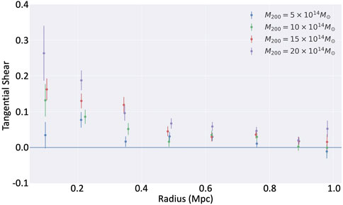
Figure 6. Azimuthally averaged tangential shear in different annular bins (eight bins ranging from 0 to 1.0 Mpc). Shear is descending following the corresponding NFW profile. At a given radius of the annulus, a higher cluster virial mass produces a larger tangential shear.

If we take the average tangential ellipticity within a fixed aperture, the value of $⟨e_{\text{tan}}⟩$ is expected to be approximately proportional to the cluster virial mass at the weak lensing limit. Hence, we plot $⟨e_{\text{tan}}⟩$ measured within apertures of 0.25 Mpc, 0.5 Mpc, and 1.0 Mpc for different cluster mass values, as shown in Figure 7. The 1.0-Mpc aperture plot presents a linear relation between $⟨e_{\text{tan}}⟩$ and all four mass values, while for 0.25 and 0.5 Mpc apertures the linearity breaks for larger $M_{200}$ $(15\hspace{0.17em}\hspace{0.17em}and\hspace{0.17em}\hspace{0.17em}20\times 10^{14}{M}_{\odot })$. The figure is consistent with the expectation that the shape measurement is biased by strong lensing signals at a small aperture that covers the central sky area of the foreground galaxy cluster. In a realistic host dark matter halo, a larger mass can cause more distorted arcs due to strong lensing around the cluster center, which is also a factor affecting shear measurements. In the shear calibration using grid simulations, this factor contributes to the non-linearity and needs to be taken into account when calibrating the measured tangential reduced shear.

Figure 7

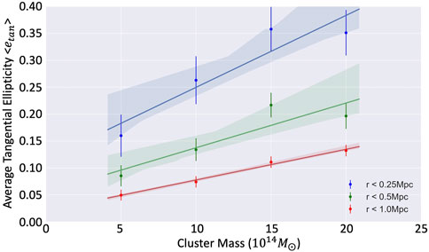
Figure 7. Average tangential ellipticities measured within given apertures (0.25, 0.5, and 1.0 Mpc) for different cluster masses. The linearity between $⟨e_{\text{tan}}⟩$ and $M_{200}$ is true for the largest aperture but unavailable in smaller apertures with larger cluster mass. The solid lines are linearly fitting for data points corresponding to each aperture. The shaded bands represent the uncertainties.

The shear at the innermost radius shows the characteristic saturation of the ellipticity demonstrated in Figure 5, whereas at larger radii, the average shear scales linearly with mass. This suggests a strategy in which cluster masses are calibrated using the signal outside of 250 kpc, corresponding to reduced shear $g_{\text{tan}}=0.3$, which is very similar to the conclusion from the grid simulations.

From the cluster simulations, the shear measurement in the LSST Science Pipelines provides a promising trend in the weak lensing regime, taking deblending and PSF modeling into account. On the other hand, if the sky area being used for measurement contains strong lensing signals, the measured shear can be biased because the strong lensed galaxies can be measured as a more circular source with a much lower tangential ellipticity than the true values. Other possible uncertainty sources in processing and analyzing procedures are discussed in Section 7.

6.2 Mass estimates

Using the pzmassfitter code, we reconstruct the convergence map and estimate the mass for the cluster, as introduced in Section 4.5. Figure 8 displays the reconstructed convergence maps of the cluster simulation shown in Figure 3. No a priori fiducial position of the foreground cluster is required. In the E-mode signal-to-noise (S/N) map shown in the left panel, the primary peak saturates at $(x,y)=(\mathrm{1786,1786})$. Given that the full field of view has $\mathrm{3,542}\times \mathrm{3,542}$ pixels, the primary peak is in good agreement with the actual cluster center, which is located at $(x,y)=(\mathrm{1771,1771})$. Because the weak lensing distortion is always in the tangential direction with respect to the galaxy cluster center, theoretically, it creates no net B-mode signal in the environment setup of our simulations. The B-mode map, shown in the right panel, may therefore be used as a null test to track potential systematic errors. Some minor clumps present in the northeast and southwest corners are likely due to measurement fluctuations and random noise. In practice, these signals are too far from the cluster center to affect the measurements.

Figure 8

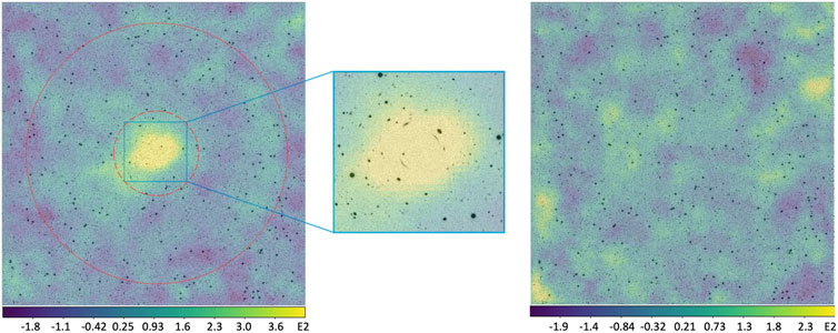
Figure 8. Reconstructed gravitational lensing convergence maps for one cluster simulation with $M_{200}=20\times 10^{14}{M}_{\odot }$ in 10-year depth. Left: E-mode S/N map of the full $12.2^{\prime }\times 12.2^{\prime }$ field of view, with a zoomed-in $2.3^{\prime }\times 2.3^{\prime }$ area. The map peaks at the center of the image, which is consistent with the actual cluster center. The red dashed and dotted circles represent the inner and outer radii of the effective region for choosing galaxies, respectively. Right: B-mode S/N map of the same sky area.

In the design of the cluster simulations, foreground galaxy clusters are placed at $z=0.3$, and all the background galaxies share the same redshift at $z=1.5$. To estimate the cluster mass, we first generate a Dirac-like $P(z)$ for each galaxy in the catalog. Coupled with the individual shapes measured by the LSST Science Pipelines and the known location and redshift of the cluster, the output measurement data are processed by pzmassfitter. To reduce the shape noise, the galaxy postage stamps are rotated by $90°$ individually at the beginning of the simulation to generate a parallel set of images. The measurements of the “original images” and “90-degree images” are combined at the level of src catalog as a separate input sample. For each group of an input $M_{200}$ value, we generate 10 cluster simulations together with their 90-degree pairs. We take the average of the mass estimates from the simulations in each group.

To illustrate the improvements from our shear calibration results, as shown in Section 5, we apply the third-order calibration (Eq. 32) to the shape measurement results and compare mass estimates with and without shear calibration.

Results are summarized in Table 2 and shown in Figure 9, for $5\times 10^{14}{\mathrm{M}}_{\odot }$ (first row), $10\times 10^{14}{\mathrm{M}}_{\odot }$ (second row), $15\times 10^{14}{\mathrm{M}}_{\odot }$ (third row), and $20\times 10^{14}{\mathrm{M}}_{\odot }$ (last row) cluster simulations. Histograms correspond to the dispersion of the posterior distribution of the reconstructed cluster mass $M_{200}$. The ground truth of cluster mass is represented by the gray vertical line, while the red vertical line gives the average of the maximum-likelihood mass estimates over the 10 simulations. The left column shows mass estimates in the absence of shear calibration, while the right column indicates results with calibrated shape measurements.

Table 2

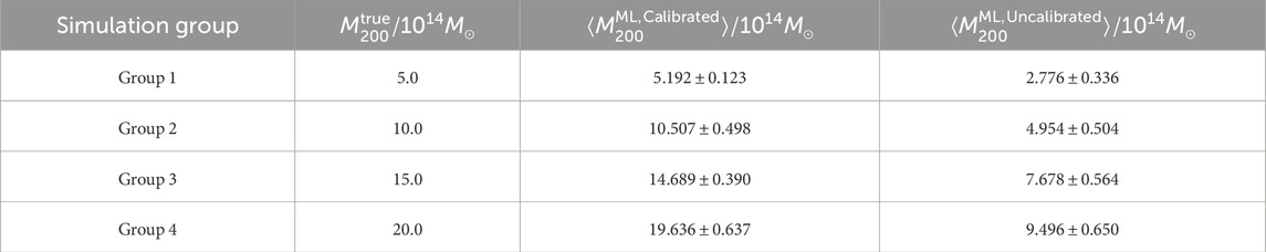
Table 2. Comparison between true virial masses of cluster simulations and average mass estimates with maximum-likelihood. The third column is the mass estimate after applying calibration on the shape measurement, while the fourth column is before calibration.

Figure 9

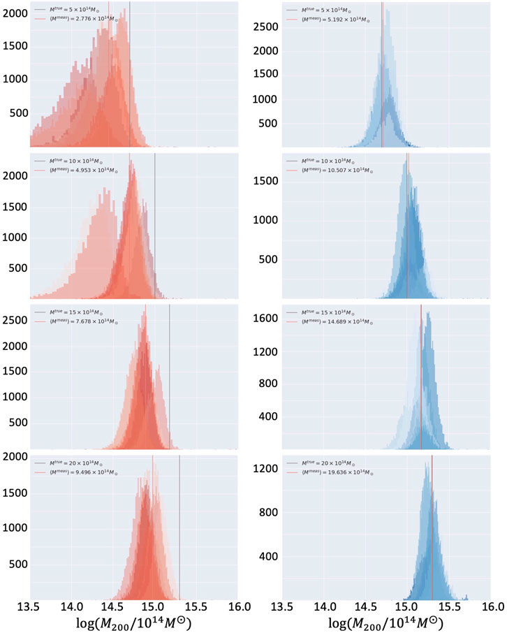
Figure 9. Likelihood distributions of mass estimates for cluster simulations, whose true virial mass values are $\mathrm{5,10,15},and20\times 10^{14}{M}_{\odot }$, respectively. These true mass values are indicated by the gray vertical solid lines. Each histogram (with a y-axis unit of counts) shows the dispersion of the maximum-likelihood over samples of $90°$ pair combined at the catalog level. The red vertical solid lines are the average of maximum-likelihood mass estimates of all samples within each panel. The left column shows results without shear calibration. The right column indicates the mass estimates after shear calibration.

Since the fitted calibration relation covers up to $g=0.4$, which approximately corresponds to a radius of 200 to 1000 kpc in our simulations, a radial cutoff of 250 kpc is applied to all mass estimations. Discussions regarding the radial cut can be found in Section 7 and Applegate et al. (2014).

As shown in Table 2 and the right four panels of Figure 9, the true mass values after calibration in all cases are close to the average maximum-likelihood mass estimates. The probability distributions also show good concentration for the true mass values. Given the fact that each cluster simulation has a finite number of background galaxies, it is possible to observe some outliers in the mass distributions. Hence, there may be some fluctuations in the peaks of the probability distributions, which is acceptable and reasonable.

The results in the left four panels of Figure 9 have significant underestimates in cluster mass. As a reference, the average maximum-likelihood mass estimate from 10 simulation realizations is compared with the corresponding true mass value in each panel. We notice that the difference between these two values increases with the true mass. The explanation is that, given a radial cutoff of 250 kpc, a stronger gravitational lensing signal is included as the cluster mass goes up to $20\times 10^{14}{\mathrm{M}}_{\odot }$. Therefore, the measured shear is underestimated in the simulations with a more massive cluster, as shown in Figure 5. These probability distributions show good agreement with our results from Section 5, and the underestimates are remarkably improved by shear calibration.

Based on these comparisons of results before and after shear calibration, we claim that the third-order calibration proves the expected improvements in the mass estimate results. More discussion regarding the uncertainties is included in Section 7.

7 Discussions on systematics

During the process of generating simulations and measuring shapes, we aim to recover factors close to realistic situations (e.g., galaxy postage stamps, lensing algorithm, PSF, and sky noise). However, there are different types of systematics introduced that we expect to understand:

• Sample size: In jedisim, for now, we have 738 galaxy postage stamps as the input database. We select these galaxies from HST UDF and CANDELS by visual inspection to ensure a variety of shapes. In the simulation procedure, the galaxy postage stamps are assigned different parameters. In addition, the shape noise is suppressed by incorporating the $90°$-rotated pairs. However, it is still necessary and helpful to add more galaxy postage stamps to the database.

• PSF: The simulated images are convolved with a uniform PSF kernel which is produced by PhoSim and characterized with parameters of LSST. In this way, the measurement biases due to PSF anisotropy and varying seeing are artificially removed. Ideally, the LSST Science Pipelines can conduct PSF correction accurately so that the shape measurements are effectively similar to our simulations. It is practical to make the PSF more realistic by feeding the simulated images into PhoSim directly instead of convolution.

• Deblending: The procedure of deblending is also simplified, given the fact that an NFW halo of pure dark matter is employed as the foreground cluster. On one hand, the absence of blending in grid simulations eliminates the systematics caused by the deblender in the LSST Science Pipelines. On the other hand, although the shape measurement in cluster simulations shows the expected trend, it is not realistic to exclude foreground–background blendings. We are making efforts to interpret the bias due to blending on lensed background sources.

• Sample characteristics: The simulations place the lens and source planes at fixed redshifts of $z=0.3\mathrm{a}\mathrm{n}\mathrm{d}1.5$, respectively. In practice, jedisim is capable of assigning and producing planes at different redshifts, which enables us to evaluate the same pipeline with a more realistic galaxy redshift distribution. In addition, the images are in a single band for now such that the LSST Science Pipelines is not able to determine the photometric redshift for each source. An improvement can be implemented in the near future by generating multi-band simulations.

In our simulations, the magnitude obeys a single power-law function for simplification, which is not the most accurate description of the magnitude according to the shear calibration results from the Kilo-Degree Survey (KiDS) (Conti et al., 2016). Although this factor does not have a dramatic impact on the shape measurement, it is reasonable to adopt more accurate functions to describe the magnitude distribution in the future.

The accuracy of the concentration parameter in the NFW profile is crucial for precise modeling of the mass distribution in galaxy clusters. The concentration parameter in this work is simplified when constructing the simulations. Systematic errors, such as PSF distortions, noise, and intrinsic shape noise, can propagate into shear calibration and subsequently affect the accuracy of the concentration parameter. We acknowledge that inaccuracies in shape measurements can introduce biases in the estimation of the concentration parameter. To mitigate these effects, more advanced shape measurement algorithms and rigorous shear calibration should be studied and employed in the future.

• Single-lens-plane assumption: In this work, we adopt the single-lens-plane assumption for our lensing simulations. This simplification allows us to focus on the lensing effects of the primary galaxy cluster while maintaining computational efficiency. However, it is important to acknowledge that this assumption does not account for the impact of additional structures along the line of sight, where these line-of-sight structures can boost the lensing cross-section (Li et al., 2019, 2021). Consequently, our results may underestimate the true lensing effects, particularly in scenarios where significant mass is distributed along the line of sight. This limitation should be considered when interpreting the results presented in this paper.

In future work, we plan to address the limitations of the single-lens-plane assumption by incorporating the effects of line-of-sight structures into our lensing simulations. This will involve the development of multi-plane lensing models that account for additional mass distributions along the line of sight. By doing so, we aim to achieve a more accurate representation of the lensing cross-section and improve the precision of our shear calibration and shape measurement results. These efforts will enhance our understanding of the mass distribution in galaxy clusters and the contribution of line-of-sight structures to the overall lensing signal.

• Mass estimate: Parameters in the pzmassfitter code are set to default, where an inner radial cut is applied on the catalogs to exclude strong lensing signals around the cluster center. We set the radial cutoff to 250 kpc, and more discussions can be found in the Weighing the Giants project (Applegate et al., 2014). It is necessary to adjust and optimize these configurations as the next step. Meanwhile, the convergence map in Figure 8 shows fluctuations in the simulated images, which are unavoidable. As the virial mass drops to $5\times 10^{14}{M}_{\odot }$, the signal-to-noise can be lower and rendered by the noise level. Given the fact that each sub-panel in Figure 9 is based on one pair of cluster simulations, it is logical to observe a skewness to low mass for the smallest cluster and high accuracy for the most massive cluster. A promising solution is to stack measurement catalogs for multiple simulations with the same cluster mass so that a larger sample can be analyzed by the MCMC algorithm to obtain more concentrated mass estimate distributions.

8 Conclusion and future work

We introduce the image simulation pipeline jedisim and generate simulation images of gravitational lensing at the scale of galaxy clusters. jedisim uses galaxy postage stamps extracted and cleaned from HDF/UDF and GOODS in CANDELS. The postage stamps are scaled to the assigned magnitude and half-light radius of each one, matching observations in HDF/GOODS, and rotated randomly before being traced through a mass distribution to construct full distortion, including both weak and strong lensing instances. Then, the lensed galaxies are convolved with a PSF kernel characterized by LSST parameters generated by PhoSim.

Cluster simulations with a size of $12.2^{\prime }\times 12.2^{\prime }$ ($\mathrm{3,542}\times \mathrm{3,542}$ pixels at the LSST resolution) are created and rendered with noise in both 1-year and 10-year survey depths. The virial mass of each cluster is $\mathrm{5,10,15},and20\times 10^{14}{M}_{\odot }$, respectively, and the concentration is 4.0. In addition, 410 grid-layout simulations are generated, each of which has a given reduced shear $g$ throughout all galaxies in it. The value of $g$ ranges from 0.02 to 0.60.

Both the cluster and grid simulations are processed and measured using LSP software stack with the obs_file package. After processing the images, the adaptive moments and ellipticities are measured for background sources using the HSM algorithm. Given the fiducial position of the cluster center, the tangential reduced shear can be calculated for background galaxies.

In the grid simulations, biases due to PSF correction and deblender of the LSST Science Pipelines are artificially constrained so that shape measurements are relatively purified. We compare and plot the measured reduced shear $g_{\text{tan}}^{\text{meas}}$ against the true reduced shear $g_{\text{tan}}^{\text{true}}$ in Figure 5. Therefore, we derive the shear calibration from the second-order and third-order polynomial fitting. The multiplicative and additive shear calibration biases of the HSM algorithm in STEP2 are adopted to construct an empirical formula as a reference. The results are consistent with the empirical formula up to $g_{\text{tan}}^{\text{true}}\lesssim 0.06$, followed by an increasing discrepancy as shear ascends. This phenomenon can be explained by the biased shape measurement for strong lensed galaxies. Meanwhile, the LSST Science Pipelines provide expected performance on shape measurement for weak lensing signals.

In the cluster simulations, by choosing different $M_{200}$ values and varying measurement apertures, the measured reduced shear shows proportionality with $M_{200}$ for an aperture dominated by the weak lensing signal. The linearity breaks as the aperture shrinks to the strong lensing regime as expected.

We plot convergence maps for the cluster simulations. The E-mode convergence map shows a reasonable mass distribution and locates the primary peak in agreement with the actual cluster center. The B-mode map plots more randomly distributed voids in the same sky area, as expected.

The output source catalogs from the LSST Science Pipelines are processed by the pzmassfitter code to estimate the maximum-likelihood cluster mass. The distributions of mass estimates from the MCMC realizations of the shear field for our simulated galaxy clusters demonstrate how the LSST Science Pipelines measurements can reliably recover cluster masses. The comparison between mass estimates before and after applying the shear calibration results from the grid simulations proves the improvement. It demonstrates that the LSST Science Pipelines can be used to probe the lensing signal in a cluster at 250 kpc from the center, increasing the sample of clusters for which individual lensing signals can be measured dramatically.

In general, to produce more realistic cluster simulations, we plan to build a larger repository of galaxy postage stamps, which is in accordance with the morphology and magnitude distribution of observations. Meanwhile, multi-band images are necessary for evaluating photometric redshift calibration and forced photometry components in the LSST Science Pipelines. In the near future, we plan to double the current sample size of galaxy postage stamps in the F450W, F606W, and F814W bands. The source galaxies are supposed to be placed at different redshifts, and a more sophisticated PSF model can be constructed by feeding the simulated images at HST resolution directly into PhoSim instead of the current convolution algorithm.

The cluster galaxies are also to be added so that the corresponding effects due to deblending can be studied. As described by Fu et al. (2019), we adopt a semi-analytic halo model to distribute foreground galaxies. As the next step, we plan to construct a more realistic lensing plane from the smoothed particle hydrodynamics simulations (Aardwolf et al., 2019) and simulate the cluster galaxies according to the CosmoDC2 extra-galactic catalogs (Korytov et al., 2019).

We hope that this work will be helpful in the shear calibration of cluster gravitational lensing and provide feedback on relevant component developments in the LSST Science Pipelines. The upcoming LSST will measure strong and weak lensing signals in the largest and most uniform sample to date of thousands of galaxy clusters. Given the requirement of high accuracy on shear measurements, it is important to determine a feasible scope and calibrate the shear measurement. Furthermore, these measurements are combined to constrain mass profiles and mass distribution in galaxy clusters and also provide a powerful probe of cosmology.

Data availability statement

The datasets presented in this study can be found in online repositories. The names of the repository/repositories and accession number(s) can be found in the article/Supplementary Material.

Author contributions

BL: writing–original draft, writing–review and editing, conceptualization, data curation, formal analysis, methodology, software, validation, and visualization. ID: writing–original draft, writing–review and editing, conceptualization, data curation, formal analysis, funding acquisition, investigation, methodology, project administration, resources, software, and supervision. NC: validation, writing–review and editing, software, methodology, and writing–original draft. DC: methodology, supervision, project administration, conceptualization, investigation, resources, writing–original draft, and writing–review and editing.

Funding

The author(s) declare that financial support was received for the research, authorship, and/or publication of this article. This work was supported by the DOE grant DE-AC02-76SF00515. This research was conducted using computational resources and services at the Center for Computation and Visualization, Brown University. This work is based on observations taken by the CANDELS Multi-Cycle Treasury Program with the NASA/ESA HST, which is operated by the Association of Universities for Research in Astronomy, Inc., under NASA contract NAS5-26555.

Acknowledgments

The authors thank the referees for their comments on this paper. They thank Daniel Parker for his fundamental contribution to the development of the first version of jedisim and Céline Combet for her substantial guidance in the usage of pzmassfitter. They express their gratitude to the LSST Data Management team for their guidance in utilizing software. BL expresses gratitude to Simon Krughoff, Dominique Boutigny, James Bosch, and Robert Lupton for their helpful comments and discussions. BL expresses gratitude to the members of the Observational Cosmology, Gravitational Lensing, and Astrophysics Research Group at Brown University for their support.

Conflict of interest

The authors declare that the research was conducted in the absence of any commercial or financial relationships that could be construed as a potential conflict of interest.

Publisher’s note

All claims expressed in this article are solely those of the authors and do not necessarily represent those of their affiliated organizations, or those of the publisher, the editors, and the reviewers. Any product that may be evaluated in this article, or claim that may be made by its manufacturer, is not guaranteed or endorsed by the publisher.

Supplementary Material

The Supplementary Material for this article can be found online at: https://www.frontiersin.org/articles/10.3389/fspas.2024.1411810/full#supplementary-material

Footnotes

¹https://www.lsst.org

²http://hsc.mtk.nao.ac.jp

³http://dm.lsst.org

⁴https://github.com/rbliu/jedisim

⁵http://www.het.brown.edu/people/ian/ClustersChallenge

⁶https://www.lsst.org/scientists/simulations/phosim

⁷https://github.com/SimonKrughoff/obs_file

⁸https://github.com/nicolaschotard/Clusters

References

Aardwolf, A., Boutigny, D., Daniel, S., Heitmann, K., Kovacs, E., Mao, Y., et al. (2019). The lsst desc dc2 simulated sky survey. Astrophysical J. Suppl. doi:10.3847/1538-4365/abd62c

CrossRef Full Text | Google Scholar

Albrecht, A., Bernstein, G., Cahn, R., Freedman, W. L., Hewitt, J., Hu, W., et al. (2006). Report of the dark energy task force. arXiv:astro-ph/0609591 ArXiv: astro-ph/0609591.

Google Scholar

Applegate, D. E., von der Linden, A., Kelly, P. L., Allen, M. T., Allen, S. W., Burchat, P. R., et al. (2014). Weighing the giants - iii. methods and measurements of accurate galaxy cluster weak-lensing masses. Mon. Notices R. Astronomical Soc. 439, 48–72. doi:10.1093/mnras/stt2129

CrossRef Full Text | Google Scholar

Beckwith, S. V. W., Stiavelli, M., Koekemoer, A. M., Caldwell, J. A. R., Ferguson, H. C., Hook, R., et al. (2006). The hubble ultra deep field. Astronomical J. 132, 1729–1755. doi:10.1086/507302

CrossRef Full Text | Google Scholar

Benitez, N., Ford, H., Bouwens, R., Menanteau, F., Blakeslee, J., Gronwall, C., et al. (2004). Faint galaxies in deep advanced Camera for surveys observations. Astrophysical J. Suppl. Ser. 150, 1–18. doi:10.1086/380120

CrossRef Full Text | Google Scholar

Bernstein, G. M., and Jarvis, M. (2002a). Shapes and shears, stars and smears: optimal measurements for weak lensing. Astronomical J. 123, 583–618. doi:10.1086/338085

CrossRef Full Text | Google Scholar

Bernstein, G. M., and Jarvis, M. (2002b). Shapes and shears, stars and smears: optimal measurements for weak lensing. Astronomical J. 123, 583–618. doi:10.1086/338085

CrossRef Full Text | Google Scholar

Bertin, E. (2013). Psfex: point spread function extractor. Astrophys. Source Code Libr. , ascl 1301, 001.

Google Scholar

Bosch, J., Armstrong, R., Bickerton, S., Furusawa, H., Ikeda, H., Koike, M., et al. (2017). The hyper suprime-cam software pipeline. arXiv:1705.06766 [astro-ph] ArXiv: 1705.06766.

Google Scholar

Bridle, S., Balan, S. T., Bethge, M., Gentile, M., Harmeling, S., Heymans, C., et al. (2010). Results of the great08 challenge: an image analysis competition for cosmological lensing. Mon. Notices R. Astronomical Soc. 405, 2044–2061. doi:10.1111/j.1365-2966.2010.16598.x

CrossRef Full Text | Google Scholar

Bridle, S., Shawe-Taylor, J., Amara, A., Applegate, D., Balan, S. T., Berge, J., et al. (2009). Handbook for the great08 challenge: an image analysis competition for cosmological lensing. Ann. Appl. Statistics 3, 6–37. doi:10.1214/08-aoas222

CrossRef Full Text | Google Scholar

Coe, D., Benitez, N., Sanchez, S. F., Jee, M., Bouwens, R., and Ford, H. (2006). Galaxies in the hubble ultra deep field: I. detection, multiband photometry, photometric redshifts, and morphology. Astronomical J. 132, 926–959. doi:10.1086/505530

CrossRef Full Text | Google Scholar

Collaboration, P., Aghanim, N., Akrami, Y., Alves, M., Ashdown, M., Aumont, J., et al. (2020). Planck 2018 results. A&A 641, A7. doi:10.1051/0004-6361/201935201

CrossRef Full Text | Google Scholar

Conti, I. F., Herbonnet, R., Hoekstra, H., Merten, J., Miller, L., and Viola, M. (2016). Calibration of weak-lensing shear in the kilo-degree survey. Mon. Notices R. Astronomical Soc., stx200. doi:10.1093/mnras/stx200

CrossRef Full Text | Google Scholar

Fahlman, G. G., Kaiser, N., Squires, G., and Woods, D. (1994). Dark matter in ms1224 from distortion of background galaxies. Astrophysical J. 437, 56. doi:10.1086/174974

CrossRef Full Text | Google Scholar

Fischer, P., and Tyson, J. A. (1997). The mass distribution of the most luminous x-ray cluster rxj1347.5-1145 from gravitational lensing. Astronomical J. 114, 14. doi:10.1086/118447

CrossRef Full Text | Google Scholar

Fu, S., Liu, B., Parker, D., and Dell’Antonio, I. (2019). Effects of blending on cluster shear profiles. Review.

Google Scholar

Grogin, N. A., Kocevski, D. D., Faber, S. M., Ferguson, H. C., Koekemoer, A. M., Riess, A. G., et al. (2011). enCandels: the cosmic assembly near-infrared deep extragalactic legacy survey. Astrophysical J. Suppl. Ser. 197, 35. doi:10.1088/0067-0049/197/2/35

CrossRef Full Text | Google Scholar

Heymans, C., Van Waerbeke, L., Bacon, D., Berge, J., Bernstein, G., Bertin, E., et al. (2006). The shear testing programme - i. weak lensing analysis of simulated ground-based observations. Mon. Notices R. Astronomical Soc. 368, 1323–1339. doi:10.1111/j.1365-2966.2006.10198.x

CrossRef Full Text | Google Scholar

Hirata, C., and Seljak, U. (2003). Shear calibration biases in weak-lensing surveys. Mon. Notices R. Astronomical Soc. 343, 459–480. doi:10.1046/j.1365-8711.2003.06683.x

CrossRef Full Text | Google Scholar

Huff, E., and Mandelbaum, R. (2017). Metacalibration: direct self-calibration of biases in shear measurement. arXiv:1702.02600 [astro-ph] ArXiv: 1702.02600.

Google Scholar

Iovino, A., Cucciati, O., Scodeggio, M., Knobel, C., Kovač, K., Lilly, S., et al. (2010). The zcosmos redshift survey: how group environment alters global downsizing trends. Astronomy Astrophysics 509, A40. doi:10.1051/0004-6361/200912558

CrossRef Full Text | Google Scholar

Jarvis, M., Bernstein, G. M., Fischer, P., Smith, D., Jain, B., Tyson, J. A., et al. (2003). Weak-lensing results from the 75 square degree cerro tololo inter-american observatory survey. Astronomical J. 125, 1014–1032. doi:10.1086/367799

CrossRef Full Text | Google Scholar

Joudaki, S., Cooray, A., and Holz, D. E. (2009). Weak lensing and dark energy: the impact of dark energy on nonlinear dark matter clustering. Phys. Rev. D. 80, 023003. doi:10.1103/physrevd.80.023003

CrossRef Full Text | Google Scholar

Jurić, M., Kantor, J., Lim, K.-T., Lupton, R. H., Dubois-Felsmann, G., Jenness, T., et al. (2015). The lsst data management system. arXiv:1512.07914 [astro-ph] ArXiv: 1512.07914.

Google Scholar

Kaiser, N., and Squires, G. (1993). Mapping the dark matter with weak gravitational lensing. Astrophysical J. 404, 441–450. doi:10.1086/172297

CrossRef Full Text | Google Scholar

Kaiser, N., Squires, G., and Broadhurst, T. (1995). A method for weak lensing observations. Astrophysical J. 449, 460. doi:10.1086/176071

CrossRef Full Text | Google Scholar

Koekemoer, A. M., Faber, S. M., Ferguson, H. C., Grogin, N. A., Kocevski, D. D., Koo, D. C., et al. (2011). Candels: the cosmic assembly near-infrared deep extragalactic legacy survey—the hubble space telescope observations, imaging data products, and mosaics. Astrophysical J. Suppl. Ser. 197, 36. doi:10.1088/0067-0049/197/2/36

CrossRef Full Text | Google Scholar

Korytov, D., Hearin, A., Kovacs, E., Larsen, P., Rangel, E., Hollowed, J., et al. (2019). Cosmodc2: a synthetic sky catalog for dark energy science with lsst. Astrophysical J. Suppl. Ser. 245, 26. ArXiv:1907.06530 [astro-ph]. doi:10.3847/1538-4365/ab510c

CrossRef Full Text | Google Scholar

Kubo, J. M., and Dell’Antonio, I. P. (2008). A method to search for strong galaxy-galaxy lenses in optical imaging surveys. Mon. Notices R. Astronomical Soc. 385, 918–928. doi:10.1111/j.1365-2966.2008.12880.x

CrossRef Full Text | Google Scholar

Laureijs, R., Amiaux, J., Arduini, S., Augueres, J.-L., Brinchmann, J., Cole, R., et al. (2011). Euclid definition study report. arXiv preprint arXiv:1110.3193.

Google Scholar

Li, N., Gladders, M. D., Rangel, E. M., Florian, M. K., Bleem, L. E., Heitmann, K., et al. (2016). Pics: simulations of strong gravitational lensing in galaxy clusters. Astrophysical J. 828, 54. doi:10.3847/0004-637x/828/1/54

CrossRef Full Text | Google Scholar

Li, N., Gladders, M. D., Heitmann, K., Rangel, E. M., Child, H. L., Florian, M. K., et al. (2019). The importance of secondary halos for strong lensing in massive galaxy clusters across redshift. Astrophysical J. 828, 122. doi:10.3847/1538-4357/ab1f74

CrossRef Full Text | Google Scholar

Li, N., Becker, C., and Dye, S. (2021). The impact of line-of-sight structures on measuring H₀ with strong lensing time delays. MNRAS 504, 2224–2234. doi:10.1093/mnras/stab984

CrossRef Full Text | Google Scholar

LSST Science Collaboration (2009). Lsst science book, version 2.0. arXiv:0912.0201 [astro-ph] ArXiv: 0912.0201.

Google Scholar

Mandelbaum, R., Lanusse, F., Leauthaud, A., Armstrong, R., Simet, M., Miyatake, H., et al. (2017). Weak lensing shear calibration with simulations of the hsc survey. arXiv:1710.00885 [astro-ph] ArXiv: 1710.00885.

Google Scholar

Mandelbaum, R., Miyatake, H., Hamana, T., Oguri, M., Simet, M., Armstrong, R., et al. (2018). The first-year shear catalog of the subaru hyper suprime-cam subaru strategic program survey. Publ. Astronomical Soc. Jpn. 70, S25. doi:10.1093/pasj/psx130

CrossRef Full Text | Google Scholar

Mandelbaum, R., Rowe, B., Armstrong, R., Bard, D., Bertin, E., Bosch, J., et al. (2015). Great3 results i: systematic errors in shear estimation and the impact of real galaxy morphology. Mon. Notices R. Astronomical Soc. 450, 2963–3007. doi:10.1093/mnras/stv781

CrossRef Full Text | Google Scholar

Massey, R., Heymans, C., Bergé, J., Bernstein, G., Bridle, S., Clowe, D., et al. (2007). The shear testing programme 2: factors affecting high-precision weak-lensing analyses. Mon. Notices R. Astronomical Soc. 376, 13–38. doi:10.1111/j.1365-2966.2006.11315.x

CrossRef Full Text | Google Scholar

McCleary, J., dell’Antonio, I., and Huwe, P. (2015). Mass substructure in abell 3128. Astrophysical J. 805, 40. doi:10.1088/0004-637x/805/1/40

CrossRef Full Text | Google Scholar

Meneghetti, M., Natarajan, P., Coe, D., Contini, E., De Lucia, G., Giocoli, C., et al. (2016). The Frontier Fields lens modelling comparison project. Mon. Notices R. Astronomical Soc. 472, 3177–3216. doi:10.1093/mnras/stx2064

CrossRef Full Text | Google Scholar

Miller, L., Heymans, C., Kitching, T. D., van Waerbeke, L., Erben, T., Hildebrandt, H., et al. (2013). Bayesian galaxy shape measurement for weak lensing surveys - iii. application to the Canada-france-Hawaii telescope lensing survey. Mon. Notices R. Astronomical Soc. 429, 2858–2880. doi:10.1093/mnras/sts454

CrossRef Full Text | Google Scholar

Miller, L., Kitching, T. D., Heymans, C., Heavens, A. F., and van Waerbeke, L. (2007). Bayesian galaxy shape measurement for weak lensing surveys - i. methodology and a fast-fitting algorithm. Mon. Notices R. Astronomical Soc. 382, 315–324. doi:10.1111/j.1365-2966.2007.12363.x

CrossRef Full Text | Google Scholar

Narayan, R., and Bartelmann, M. (1996). Lectures on gravitational lensing. arXiv preprint astro-ph/9606001.

Google Scholar

Navarro, J. F., Frenk, C. S., and White, S. D. M. (1996). The structure of cold dark matter halos. Astrophysical J. 462, 563. doi:10.1086/177173

CrossRef Full Text | Google Scholar

Navarro, J. F., Frenk, C. S., and White, S. D. M. (1997). A universal density profile from hierarchical clustering. Astrophysical J. 490, 493–508. doi:10.1086/304888

CrossRef Full Text | Google Scholar

Peterson, J. R., Jernigan, J. G., Kahn, S. M., Rasmussen, A. P., Peng, E., Ahmad, Z., et al. (2015). Simulation of astronomical images from optical survey telescopes using a comprehensive photon Monte Carlo approach. Astrophysical J. Suppl. Ser. 218, 14. doi:10.1088/0067-0049/218/1/14

CrossRef Full Text | Google Scholar

Plazas, A. A., Meneghetti, M., Maturi, M., and Rhodes, J. (2019). Image simulations for gravitational lensing with skylens. Mon. Notices R. Astronomical Soc. 482, 2823–2832. doi:10.1093/mnras/sty2737

CrossRef Full Text | Google Scholar

Ribli, D., Dobos, L., and Csabai, I. (2019). Galaxy shape measurement with convolutional neural networks. Mon. Notices R. Astronomical Soc. 489, 4847–4859. doi:10.1093/mnras/stz2374

CrossRef Full Text | Google Scholar

Rowe, B. T., Jarvis, M., Mandelbaum, R., Bernstein, G. M., Bosch, J., Simet, M., et al. (2015). Galsim: the modular galaxy image simulation toolkit. Astronomy Comput. 10, 121–150. doi:10.1016/j.ascom.2015.02.002

CrossRef Full Text | Google Scholar

Schneider, P. (2006). Weak gravitational lensing. , arXiv:astro-ph/0509252 33, 269–451. doi:10.1007/978-3-540-30310-7_3

CrossRef Full Text | Google Scholar

Schneider, P., King, L., and Erben, T. (2000). Cluster mass profiles from weak lensing: constraints from shear and magnification information. Astronomy Astrophysics 353, 41–56.

Google Scholar

Sheldon, E. S., Becker, M. R., Jarvis, M., Armstrong, R., and Collaboration, T. L. D. E. S. (2023). Metadetection weak lensing for the vera c. rubin Obs. ArXiv:2303.03947 [astro-ph]. doi:10.48550/arXiv.2303.03947

CrossRef Full Text | Google Scholar

Sheldon, E. S., and Huff, E. M. (2017). Practical weak-lensing shear measurement with metacalibration. Astrophysical J. 841, 24. doi:10.3847/1538-4357/aa704b

CrossRef Full Text | Google Scholar

Spergel, D., Gehrels, N., Baltay, C., Bennett, D., Breckinridge, J., Donahue, M., et al. (2015). Wide-field infrarred survey telescope-astrophysics focused telescope assets wfirst-afta 2015 report. arXiv e-prints , arXiv–1503.

Google Scholar

Tewes, M., Kuntzer, T., Nakajima, R., Courbin, F., Hildebrandt, H., and Schrabback, T. (2019). enWeak-lensing shear measurement with machine learning: teaching artificial neural networks about feature noise. Astronomy Astrophysics 621, A36. ArXiv:1807.02120 [astro-ph, stat]. doi:10.1051/0004-6361/201833775

CrossRef Full Text | Google Scholar

Van Waerbeke, L., and Mellier, Y. (2003). Gravitational lensing by large scale structures: a review. arXiv:astro-ph/0305089 ArXiv: astro-ph/0305089.

Google Scholar

Voigt, L. M., and Bridle, S. L. (2010). Limitations of model-fitting methods for lensing shear estimation. Mon. Notices R. Astronomical Soc. 404, 458–467. doi:10.1111/j.1365-2966.2010.16300.x

CrossRef Full Text | Google Scholar

Wright, C. O., and Brainerd, T. G. (2000). Gravitational lensing by nfw halos. Astrophysical J. 534, 34–40. doi:10.1086/308744

CrossRef Full Text | Google Scholar

Zhang, Z., Shan, H., Li, N., Wei, C., Yao, J., Ban, Z., et al. (2024). FORKLENS: accurate weak-lensing shear measurement with deep learning. Astronomy Astrophysics 683, A209. ArXiv:2301.02986 [astro-ph]. doi:10.1051/0004-6361/202345903

CrossRef Full Text | Google Scholar