Simulated gravity field estimation for Deimos based on spacecraft tracking data

An accurate gravity field model of Deimos can provide constraints for its internal structure modeling, and offer evidence for explaining scientific issues such as the origin of Mars and its moons, and the evolution of the Solar System. The Japanese Martian Moon Exploration (MMX) mission will be launched in the coming years, with a plan to reach Martian orbit after 1 year. However, there is a lack of executed missions targeting Deimos and research on high-precision gravity field of Deimos at this stage. In this study, a 20th-degree gravity field model of Deimos was constructed by scaling the gravity field coefficients of Phobos and combining them with an existing low-degree gravity field model of Deimos. Using simulated ground tracking data generated by three stations of the Chinese Deep Space Network, we simulate precise tracking of a spacecraft in both flyby and orbiting scenarios around Deimos, and the gravity field coefficients of Deimos have been concurrently computed. Comparative experiments have been conducted to explore factors affecting the solution, indicating that the spacecraft’s orbital altitude, the noise level of observation data, and the ephemeris error of Deimos have a significant impact on the solution results. The results of this study can provide references for planning and implementation of missions targeting Martian moons.

1 Introduction

Among the two natural satellites of Mars, Deimos is the smaller one and is further from Mars than Phobos. Traces of the formation and evolution processes on the surface of Mars are not obvious, while the surfaces of the Martian satellites are relatively primitive. Studying the mass, shape, gravity field model, rotation parameters, and internal structure of Deimos can provide a foundation for deducing the formation and evolution of both Deimos and Mars. Furthermore, this may serve as an effective approach to addressing scientific questions such as the formation and evolution of the Earth and the Solar System (Gao et al., 2021b). Additionally, Deimos, with its favorable position and weak gravitational field, allows spacecraft to orbit at relatively low altitudes (Sagdeev and Zakharov, 1989). In the future, it could serve as a bridge and supply station for human exploration into deep space (Guo et al., 2020).

Since Asaph Hall’s discovery of Deimos in 1877, humanity has engaged in exploration activities using various methods such as ground observations, the Hubble Telescope, and deep space spacecrafts (Tieying et al., 2021). Especially after the 1970s, various Mars and deep space spacecrafts have been launched, conducting more in-depth investigations of Deimos (Yang et al., 2019). However, there are currently no confirmed exploration missions solely focused on Deimos. Most studies and observations of Deimos have relied on data obtained by spacecrafts during Mars missions. NASA’s Mariner nine spacecraft captured images of Deimos, with the closest distance being 1,200 km and achieving a resolution of 30 m (Cutts, 1974). The Viking 2 orbiter conducted five flyby observations of Deimos, with the closest observation distance being 33 km (Williams and Friedlander, 2015). The European Space Agency’s Mars Express mission (MEX) utilized a high-resolution stereo camera and an imaging spectrometer to reevaluate the volume and density of Deimos and study its surface composition based on observation data (Witasse et al., 2014). NASA’s Mars Reconnaissance Orbiter (MRO) captured the first color high-resolution images of Deimos using the High-Resolution Imaging Science Experiment (HiRISE) camera (Dunbar, 2009). Table 1 summarizes the current knowledge of the orbital parameters and physical properties of Deimos (Tieying et al., 2021) used for our simulation.

Table 1

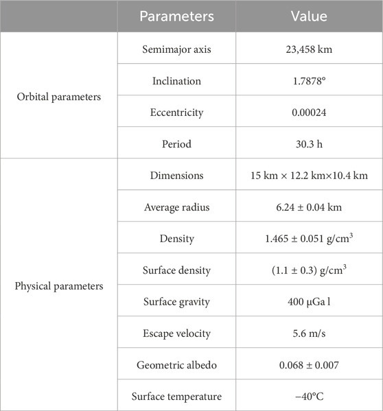
Table 1. The orbital and physical parameters of Deimos.

As one of the two natural satellites of the Earth-like planets in the Solar System, Deimos is attracting more and more attention in the field of deep space exploration. NASA has organized three international conferences on the exploration of Phobos and Deimos (Lee, 2016). Chinese Tianwen-1 spacecraft will conduct further exploration, with potential targets being Phobos and Deimos (Liu et al., 2023). The MMX mission by the Japan Aerospace Exploration Agency (JAXA) was originally scheduled to launch in 2024 and arrive in Martian orbit in 2025 (Kuramoto et al., 2018). It is expected to conduct close-range exploration to the Martian moons, with one of the mission objectives being to calculate the high-degree gravity field of Deimos (Nakamura et al., 2021).

The ephemeris and gravity field of planetary satellites serve as crucial references for the orbit design and planning of planetary satellite exploration missions. The high-precision ephemeris and gravity field of Deimos can ensure the precise entry of the spacecraft into the gravitational influence area of Deimos, thus enabling the implementation of challenging maneuvers such as flyby and orbit insertion (Guo et al., 2020). Currently, there are mainly two methods for calculating the gravity field models of celestial bodies in deep space exploration. The first method is to forward generate the gravity field model of the celestial body based on its precise shape model and a certain density assumption. The second method utilizes close-range orbit tracking data from the spacecraft to extract perturbation information and inversely derive the gravity field model of the celestial body. Method one was employed in Yamamoto et al. (2023) and Guo et al. (2020) for modeling the gravity field of Phobos, while method two was used in Yang et al. (2019) for modeling the gravity field of Phobos. Rubincam et al. (1995) used method one to compute the 4th-degree gravity field of Deimos. However, due to the lack of completed exploration missions specifically targeting Deimos, existing studies and literature on Martian moons predominantly focus on Phobos. Deimos is only briefly mentioned in most Mars satellite research and literature, as seen in the papers of Yamamoto et al. (2023), Witasse et al. (2014), and Nakamura et al. (2021). Moreover, there is scarce research employing method two for modeling the gravity field of Deimos.

In response to the needs of future exploration missions and the shortcomings in current research, this study primarily conducted the following research tasks using ground station simulated radio tracking data. By scaling the gravity field coefficients of Phobos and combining them with existing low-degree gravity field model of Deimos, we constructed a 20th-degree gravity field model of Deimos, which was then tested and corrected based on Kaula criterion (Kaula and Street, 1967). We simulated precise orbit determination for the spacecraft in the flyby and orbiting scenarios. The gravity field coefficients of Deimos were inferred and evaluated for accuracy using simulated orbital data of the spacecraft. Furthermore, comparative experiments were conducted to investigate and analyze the factors affecting the gravity field determination.

2 Model and method

This paper presents our simulation based on scenarios involving the spacecraft’s flyby and orbiting around Deimos, aiming to better adapt to potential changes in the subsequent exploration plan. Based on Wuhan University’s SPOT software system (Gao et al., 2023), we developed precision orbit determination and gravity field parameter estimation software for Deimos.

Since the gravity field of Deimos is weak, the other force models acting on the spacecraft need to be accurately modeled. The inertial motion equation for the spacecraft is shown in Eq. 1:

$m\ddot{r}=f_{Mars}+f_{Deimos}+f_{NB}+f_{SRP}+f_{REL}(1)$

The model parameters for the simulation calculations are shown in Table 2.

Table 2

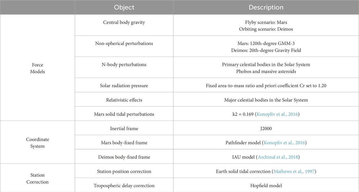
Table 2. Simulation configuration.

As shown in Table 2, in the flyby and orbiting scenarios, the forces acting on the spacecraft mainly come from Mars and Deimos. For the calculations, the recent 120th degree and order Gravity Model of Mars (GMM-3) (Genova et al., 2016) was chosen as the model for the gravitational field of Mars. In the experimental scenarios, the GM values and positions of major celestial bodies in the Solar System were obtained from the planetary ephemeris DE440 provided by the Jet Propulsion Laboratory (JPL). The state of Mars’ satellites relative to Mars and the GM value for Deimos were obtained from the JPL’s MAR097 ephemeris, with an initial GM value for Deimos set at 9.61556965e-5 km³·s^-2. The positions and GM values for large mass asteroids were provided by the sb441-n16 ephemeris from JPL’s Small-Body Database. The Chinese Deep Space Network consists of the Kashgar, Jiamusi and China-Argentina Deep Space Station, with station coordinates provided by design documents. Additionally, the average radius of Mars is considered to be 3,396 km (Genova et al., 2016). The 4th-degree gravity field of Deimos, calculated by Rubincam et al. (1995), serves as starting point for the simulation, and detailed numerical values are presented in Table A1.

This paper primarily evaluates the effectiveness and precision of gravity field recovery through spectral analysis of the gravity field. The expression for the gravitational potential function based on the spherical harmonic expansion is provided (Heiskanen and Moritz, 1976) in Eq. 2:

$V=\frac{GM}{r}{\displaystyle \sum _{n=0}^{\infty }}{\left(\frac{R}{r}\right)}^n{\displaystyle \sum _{m=0}^n}\left({\overline{C}}_{nm}\cos m\lambda +{\overline{S}}_{nm}\sin m\lambda \right){\overline{P}}_{nm}\left(\sin \phi \right)(2)$

where $G$ is the gravitational constant, $M$ is the mass of the central body, $R$ is the reference radius of the central body, $\left(r,\lambda ,\phi \right)$ are the spherical coordinates representing the radial distance, longitude, and latitude. ${\overline{C}}_{nm}$ and ${\overline{S}}_{nm}$ are the normalized spherical harmonic coefficients, where $n$ and $m$ represent the degree and order. ${\overline{P}}_{nm}\left(\sin \phi \right)$ is the normalized associated Legendre function.

For a further analysis of the gravity field determination, the accuracy of the calculated gravity field can be assessed through the power spectra, which include the rms coefficient sigma degree variances, ${\sigma }_n$ and the rms coefficient error degree variances, ${\delta }_n$ and ${\Delta }_n$. We choose the same criterion for our study. The equations for calculating these values are shown in Eqs 3–5:

${\sigma }_n=\sqrt{\frac{{\displaystyle \sum _{m=0}^n}\left({\overline{C}}_{nm}^2+{\overline{S}}_{nm}^2\right)}{2n+1}}(3)$

${\delta }_n=\sqrt{\frac{{\displaystyle \sum _{m=0}^n}\left({\sigma }_{{\overline{C}}_{nm}}^2+{\sigma }_{{\overline{S}}_{nm}}^2\right)}{2n+1}}(4)$

${\Delta }_n=\sqrt{\frac{{\displaystyle \sum _{m=0}^n}\left({\Delta }_{{\overline{C}}_{nm}}^2+{\Delta }_{{\overline{S}}_{nm}}^2\right)}{2n+1}}(5)$

Where ${\sigma }_{{\overline{C}}_{nm}}$ and ${\sigma }_{{\overline{S}}_{nm}}$ are error variances of the gravity field coefficients ${\overline{C}}_{nm}$ and ${\overline{S}}_{nm}$, respectively. ${\sigma }_n$ reflect the magnitude of each degree’s coefficients, ${\delta }_n$ and ${\Delta }_n$ serve as precision assessment indicators. Typically, the formal errors ${\delta }_n$ are retrieved from the posterior covariance matrix of the model, and will stabilize with an increasing number of observations. The true errors ${\Delta }_n$, which reflects the deviation of the calculated results from the reference/true results, are more effective in evaluating the accuracy and reliability of the calculation results.

The Kaula criterion is a statistical model used to describe the expected behavior of the coefficients in a spherical harmonic expansion of the gravity field. In simple terms, the normalized spherical harmonic coefficients exhibit a zero mean property. It states that the degree variance of these coefficients decreases inversely with the α-th power of the degree $n$. This means that higher-degree coefficients, which correspond to smaller spatial scales, are generally smaller in magnitude. The equation representing this relationship is shown in Eq. 6:

${\sigma }_n\sim 0\pm \frac{k}{n^{\alpha }}(6)$

where $k$ is the constant coefficient of the Kaula criterion curve. The introduction of the Kaula criterion in the determination of the Deimos gravity field model serves as a regularization factor to overcome the instability of solving the gravity field while providing a smoothing effect on the calculation of high-order coefficients.

Constrained by the accumulation of historical data on Deimos, the progress of Martian moon exploration missions like MMX, and the depth of related research, there is currently lack of a priori information on the high-degree and high-precision gravity field of Deimos. Considering the small mass and volume of Deimos, we constructed a 20th-degree gravity field for Deimos as the initial model for the solution. Desprats et al. (2021) constructed the 100th-degree gravity field of Callisto, the fourth moon of Jupiter, whose 3rd to 100th degree coefficients were based on the scaled Moon’s gravity field. In this study, following his approach, we obtained Deimos’ gravity field coefficients from 5th to 20th degree by scaling the coefficients of Phobos provided in Guo et al. (2020). These scaled coefficients, combined with the 4th-degree coefficients provided by Rubincam et al. (1995), formed the 20th-degree gravity field of Deimos, which would be involved in the subsequent gravity field solution for Deimos. The scaling factors were calculated based on the GM values and average radii of Phobos and Deimos, and were validated and adjusted according to Kaula criterion. Figure 1 shows the power spectra of the Deimos 20th-degree gravity field generated by scaling.

Figure 1

Figure 1. Power spectra for the 20th-degree gravity field of Deimos.

As shown in Figure 1, ${\sigma }_n$ represents the degree variances of the 20th-degree the Deimos gravity field coefficients. “Kaula4” and “Kaula20” respectively represent the Kaula curves fitted with 4th and 20th degree Deimos gravity field coefficients. The closeness of the two curves in Figure 1 indicates that the scaled initial values of the Deimos 20th-degree gravity field coefficients are reliable and could serve as a reference for subsequent simulation experiments.

After establishing a comprehensive perturbation model for the spacecraft orbit, based on the observation plan set in this study, simulations were conducted to obtain Doppler data through radio tracking observations with an elevation angle of 10° or higher. Simulated observed data, including appropriate noise, were then generated and used to construct a simulated observational dataset. The fitting and iterative refinement process aimed to minimize the sum of squared residuals (Montenbruck and Gill, 2012). Weighted least squares estimation was employed during the solution process, and the calculation equation is shown in Eq. 7:

${\mathit{x}}_{\mathbf{0}}={\left(H^{T}WH\right)}^{-1}\left(H^{T}Wy\right)(7)$

where ${\mathit{x}}_{\mathbf{0}}$ represents the estimated values of the corrections for the batch processing, $H$ is the Jacobian matrix of the parameters to be estimated, $W$ is the weight matrix of the observed values, $y$ is the residual.

The optimal estimate at the initial moment ${\widehat{\mathit{X}}}_{\mathbf{0}}$, which is also the corrected initial orbit state, can be calculated by the following equation in Eq. 8:

${\widehat{\mathit{X}}}_{\mathbf{0}}={\mathit{X}}_{\mathbf{0}}+{\mathit{x}}_{\mathbf{0}}(8)$

where ${\mathit{X}}_{\mathbf{0}}$ is the initial orbit state.

The simulated observations used in this study are two-way Doppler measurements with a sample rate of 60 s, and the default measurement noise for the observational data was set to Gaussian white noise with a standard deviation of 0.1 mm/s, which represents the precision level of current conventional X-band tracking (Sun et al., 2023). The transformation from the body-fixed coordinate system of Deimos to the inertial coordinate system followed the method recommended by IAU 2015 (Archinal et al., 2018), determined by the right ascension angle $\alpha$, declination angle $\delta$, and initial prime meridian angle $W$. For simplicity, errors in angle $\alpha$, $\delta$, and $W$ were assumed to be ±0.01° based on testing (Yang, 2023). Additionally, this study assumed an error in the time of the periapsis passage of one of Deimos’ orbital elements, as it can only be determined imprecisely through astronomical observations. Assuming an error of 0.01 s in the periapsis time at the initial epoch, this error is equivalent to magnitudes of 10 m for the initial position and 0.001 m/s for the initial velocity in Cartesian coordinates. In our computations, we added the above-mentioned errors to the initial orbit state. Following the approach in Liu et al. (2023) and assuming uniform density for the Deimos, each coefficient of the Deimos gravity field was initially perturbed by adding 0.001 times its own value, serving as the initial model for iterative computation. The uncertainties of estimated parameters were set to three times the formal errors of the solved-for parameters, and the weight matrix was determined by the formal errors.

Table 3 lists different cases considered in the orbiting Scenario to explore the impact of various factors on the determination of the spacecraft’s orbit and the solution of Deimos’ gravity field. In the comparative experiments, only the parameters in Table 3 were changed, while the remaining parameters were kept constant. To simplify calculations, the orbital altitude of the spacecraft in this paper is directly obtained by subtracting the average radius of Deimos (6.24 km) from the distance between the spacecraft and the center of Deimos.

Table 3

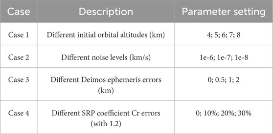
Table 3. Study cases considered in the simulation.

3 Results

3.1 Spacecraft orbit perturbation analysis

This section provides a rough estimate of the magnitudes of various perturbations, aiming to facilitate the planning of subsequent simulation exploration and observation scenarios. Figure 2 illustrates the magnitudes of accelerations provided by various perturbative forces on a spacecraft with orbital altitudes ranging from 4 to 100 km at the orbit insertion moment.

Figure 2

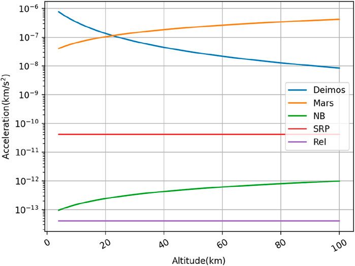
Figure 2. Acceleration magnitude with orbital altitudes ranging from 4 to 100 km.

As shown in Figure 2, during the close-range exploration of Deimos, the perturbation accelerations provided by Deimos and Mars are predominant. As the spacecraft’s orbital altitude increases from 4 to 100 km, the perturbation acceleration provided by Deimos decreases, while that provided by Mars gradually increases. Starting from an orbital altitude of about 24 km, the perturbation acceleration provided by Mars surpasses that of Deimos. Moreover, the perturbation accelerations provided by solar radiation pressure (“SRP”) and relativistic effects (“Rel”) remain almost unchanged, while those provided by natural celestial bodies (“NB”) slightly increase (mainly from Phobos).

Then, we explored the orbital characteristics of the spacecraft in such a perturbation environment. Figure 3 illustrates the magnitudes of accelerations experienced by the spacecraft in the initial orbits with altitudes of 4 km, 8 km, 12 km, and 30 km during a forward integration of 24 h in the orbiting scenario.

Figure 3

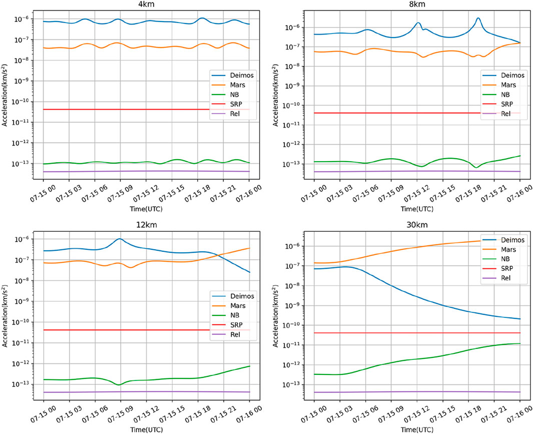
Figure 3. Acceleration magnitude of the spacecraft’s 24-h orbit in different initial orbital altitudes.

As shown in Figure 3, the accelerations caused by solar radiation pressure and general relativistic effects for orbits at different altitudes are relatively stable. However, the perturbation acceleration caused by natural celestial bodies undergoes some variations over time. When the initial orbit height is 4 km, the spacecraft can stably orbit Deimos during this period. As the orbit altitude increases, the spacecraft gradually fails to stably orbit Deimos, and it may escape from the orbit after some time of natural motion, transitioning to a state of accompanying or flyby around Deimos. Besides, orbits may also exhibit an accompanying state when the spacecraft makes a very close flyby.

After comprehensive analysis, we adopted a simulation approach based on multi-arc joint adjustment. Different arc lengths were used in the flyby and orbital scenarios to simulate and predict spacecraft’s close-distance exploration of Deimos with maximum fidelity and anticipate data quality. Additionally, in the simulation experiments, prior constraints need to be imposed on several parameters. Table 4 provides the prior constraint configurations for the estimated parameters used in this study.

Table 4

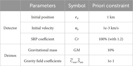
Table 4. Priori constraint settings for parameters.

As shown in Table 4, we assume that these prior constraints can be achieved before the exploration mission phase. After experimental validation, it was found that the numerical values of these prior constraints were relatively loose, with minimal impact on the theoretically calculable results and experimental conclusions. The purpose of setting prior constraints is to ensure the success rate of experimental calculations, improve computational efficiency, especially in comparative experiments.

3.2 Results in the flyby scenario

In the flyby scenario, considering Deimos’ average radius of 6.24 km and the minimum flyby distance of 33 km achieved in historical exploration missions like Viking 2, many simulations were conducted to select instances where the distance from the spacecraft to the center of Deimos falls between 32 km and 48 km. These selected moments served as the initial times for each flyby segment, with the orbital state of Deimos at these initial times being used as the initial orbit state for each segment, resulting in six simulated flyby segments.

The subsatellite point refers to the projection of a spacecraft on the surface of Deimos at a given moment. These points are directly situated along the line connecting the spacecraft and the center of Deimos. The location of the subsatellite points to some extent reflects the coverage of the spacecraft’s orbit over Deimos, which affects the precision of the solution results and the order of the gravitational field that can be solved. In Figure 4, we have depicted the distribution of the subsatellite points of the spacecraft’s orbit in the flyby scenario. We set the longitude range of the Deimos-fixed frame to be from −180° to 180°, and the latitude range to be from −90° to 90°.

Figure 4

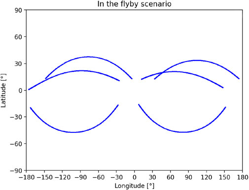
Figure 4. Distribution of spacecraft’ subsatellite points in the flyby scenario.

As shown in Figure 4, subsatellite points with an orbit altitude less than 100 km are plotted in the flyby scenario, and only their corresponding orbital data are involved in subsequent calculations. It is observed that in the flyby scenario, the subsatellite points cover a longitude range of approximately ±180°, while ±45° in latitude.

Parameters such as the initial orbit state of each segment, solar radiation pressure coefficient (Cr), etc., were considered as local parameters, while Deimos’ GM and gravity field coefficients were treated as global parameters for computation. A combined approach similar to the method described in Liu. (2022) was used for solving the normal equations, leading to the determination of Deimos gravity field through a joint adjustment. Table 5 presents partial results in the flyby scenario.

Table 5

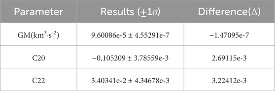
Table 5. Partial results in the flyby scenario.

As shown in Table 5, the precision of the orbit determination results, denoted by “Formal error”, and their deviation “True error” from reference values demonstrate that the calculation outcomes are favorable. This underpins the premise of the reliability in the gravitational field coefficient computation by this method. The calculation results of Deimos’ GM value and some gravitational field coefficients in this paper are consistent with those in the paper of Rubincam et al. (1995), and there was an improvement in the calculation precision. Figure 5 illustrates the power spectra of the gravity field solution for Deimos in the flyby scenario.

Figure 5

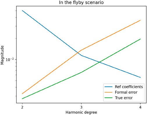
Figure 5. Power spectra of the gravity field solution in the flyby scenario.

The “Ref coefficients” in Figure 5 is equivalent to “ ${\sigma }_n$” in Figure 1, which represents the variance of the gravity field coefficients of Deimos. The trend of the power spectrum lines and their intersections indicate that only up to the 3rd-degree coefficients of the gravitational field of Deimos can be solvable and reliably estimated in the flyby scenario. In this paper, we set the maximum degree on the x-axis of the power spectra figure to the solvable degree plus 1 or 2 to highlight the solution results.

The results in Figure 5 show that, even under relatively ideal experimental conditions and with efforts to maximize the span of closer flyby data, the two-way Doppler data between ground stations and the spacecraft provided constraints only on the lower-degree coefficients of Deimos’ gravity field. The higher-degree coefficients are largely unconstrained. We speculate that this is primarily related to both spacecraft altitude and to a very sparse spatial coverage of the surface, which does not allow for highly-resolved probing of the gravity field in the flyby scenario.

3.3 Results in the orbiting scenario

If more accurate gravity field data of Deimos is required through spacecraft orbit inversion, it is necessary to consider scenarios where the spacecraft orbits around Deimos. When conducting simulation experiments in the orbiting scenario, it is considered that the spacecraft may not be able to orbit Deimos continuously and stably for a long time as the orbital altitude increases. Therefore, the adopted scheme for obtaining simulation segments was as follows. From the simulation period, 30 simulation moments spaced 12 h apart were selected. And at these moments, initial orbit state at specified orbital altitudes were generated by our design functions. We performed orbit integration separately for each set of initial orbit state for 12 h, resulting in 30 orbiting segments. Figure 6 depicts the distribution of subsatellite points in the orbiting scenario.

Figure 6

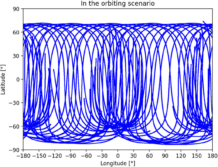
Figure 6. Distribution of spacecraft’ subsatellite points in the flyby scenario.

As shown in Figure 6, in the orbiting scenario, the subsatellite points cover a latitude range of approximately −80°–70°, while achieving full coverage in longitude. Compared to in the flyby scenario, the distribution of orbiting subsatellite points is more uniform. This indicates that the orbital data in the orbiting scenario is more effective and reliable.

Similar to in the flyby scenario, the parameters of each segment in the orbiting scenario were divided into local and global parameters for computation. The least squares method was employed to solve the gravity field of Deimos by combining the normal equations of multiple segments. Table 6 presents partial results of the gravity field of Deimos obtained in the orbiting scenario, with the spacecraft’s initial orbit altitude approximately 4 km.

Table 6

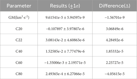
Table 6. Partial results in the orbiting scenario.

As shown in Table 6, Deimos’ calculated GM is 9.61541e-5 ± 5.94597e-9 km³·s-2, C20 is −0.107897 ± 3.97807e-6, C22 is 3.08143e-2 ± 4.60863e-6, et al. Using accuracy metrics as the evaluation criterion, the computational results in the orbiting scenario are superior to those in the flyby scenario. Figure 7 shows the corresponding results’ power spectra.

Figure 7

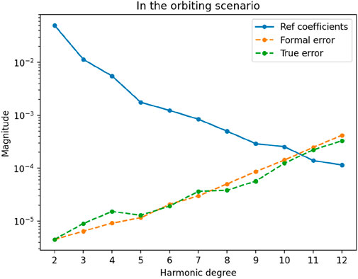
Figure 7. Power spectra of the gravity field solution in the orbiting scenario.

As shown in Figure 7, the orbit state with an initial orbit altitude of 4 km can calculate up to the 10th degree. Figures 5, 7 indicate that the accuracy of the Deimos gravity field coefficient calculation in the orbiting scenario is generally better and more stable compared to in the flyby scenario. The improvement in accuracy is particularly noticeable in the calculation of lower-degree coefficients, and can make it easier to confirm the effective degrees of the gravity model.

Additionally, Table 7 summarizes the Deimos GM calculation results from this study and selected literature. As shown in Table 7, the Deimos GM calculation results from this study are consistent with previously published findings, with significantly improved accuracy.

Table 7

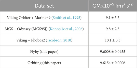
Table 7. Solutions for the gravitational constants (GM) of Deimos.

3.4 Analysis of influential factors

We adjusted the parameters outlined in Table 3 for comparative experiments and the influence of various factors on the experimental outcomes was explored. Considering that in the orbiting scenario, the precision of the calculated results significantly surpassed which in the flyby scenario, and the former demonstrated greater sensitivity to changes in influencing factors than the latter, only comparative experimental outcomes in the orbiting scenario were presented. As the formal error ${\delta }_n$ is simultaneously influenced by a substantial accumulation of observations, the coefficient error variance ${\Delta }_n$ was prioritized as the evaluation criterion.

Initially, the impact of the initial orbit altitude on the calculation outcomes was investigated. Typically, in the orbiting scenario, the spacecraft’s initial orbit altitude largely determined the range of integrated orbit altitudes. Meanwhile the integrated orbit altitudes may fall below the initial orbit altitude. Based on safety considerations and experimental validation, this study ultimately selected 4 km as the minimum simulated orbit altitude. Figure 6 illustrates the power spectra under different initial orbit altitudes.

As shown in Figure 8, it is worth noting that with the increase in the initial orbit altitude within a certain range, the perturbation force provided by Deimos decreased, while the perturbation effect from Mars gradually became more significant, leading to a gradual reduction in the accuracy of gravity field and the solvable degree of calculation. In our experiments, as the spacecraft’s initial orbit increased from 4 km to 8 km, the maximum degree of Deimos’ gravity field that could be calculated decreased by approximately 2–3°. Furthermore, due to the extremely weak gravity field of Deimos, the spacecraft may gradually fail to sustain long-term orbiting in its natural state, and may even escape Deimos’ orbit, transitioning to a state of flyby or accompanying. In fact, it can also be roughly inferred that the enhancement in calculation accuracy from the flyby scenario to the orbiting scenario primarily stemmed from the reduction in orbit altitude. Taking these factors into consideration, attention should be paid to the orbital altitude threshold when designing orbiting trajectories, with altitudes of 4–8 km above Deimos’ surface being deemed more appropriate.

Figure 8

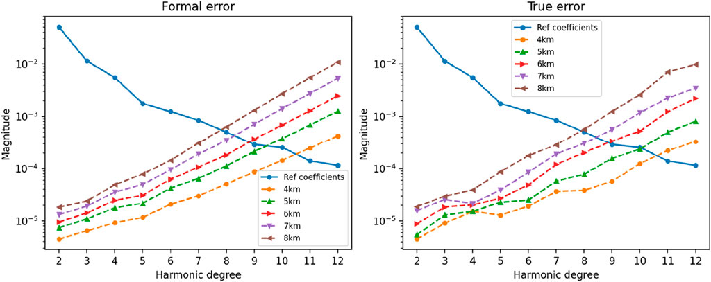
Figure 8. Power spectra in case 1 listed in Table 3 (Different initial orbital altitudes).

The observation noise determines the quality of the observation data, thereby affecting the precision of gravity field calculation results. Therefore, it was necessary to investigate the influence of observation data noise level on the calculation. In this comparative experiment, we set the observation noise level to three levels: 1e-6, 1e-7, and 1e-8 km/s Figure 7 depicted the power spectra of the calculation results obtained using observation data with different noise levels.

As shown in Figure 9, when the observation noise level decreased from 1e-6 km/s to 1e-8 km/s, the calculation precision improved by approximately five orders of magnitude. Gaussian white noise of 1e-7 km/s represented the current conventional X-band tracking precision level and was also the default level added in all other experiments. Filtering can reduce the noise level of observation data with large noise, but the ability to reduce noise level is limited by the current level of miniaturization and physical characteristics of onboard electronic devices. Therefore, the settings of 1e-6 and 1e-8 km/s noise levels were only indicative.

Figure 9

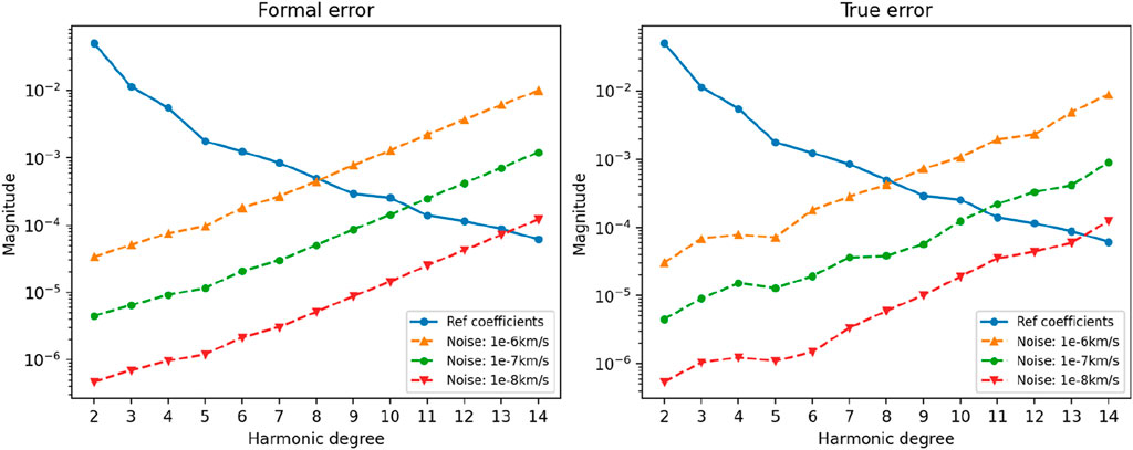
Figure 9. Power spectra in case 2 listed in Table 3 (Different noise levels).

In the simulations described above, the state of Deimos relative to Mars was directly obtained from JPL’s MAR097 ephemeris, assuming that there were no errors in the Deimos ephemeris. However, estimating the effect of ephemeris errors on parameter estimation is a crucial consideration. In the simulation experiments, following the approach of Gao et al. (2021a) and Sun et al. (2023), experiments were conducted by introducing different levels of errors along the trajectory direction of Deimos to investigate the impact of ephemeris errors. In this study, errors were introduced into the Deimos ephemerides at magnitudes of 0, 0.5, 1, and 2 km, respectively. Figure 8 illustrates the power spectra of the calculation results using Deimos ephemerides with different error magnitudes.

As shown in Figure 10, in cases where the ephemeris error is less than 0.5 km, the differences in the power spectra of gravity field coefficients are relatively small. However, in cases with ephemeris error of 1 km, deviations in the high-degree gravity field can be observed. While ephemeris error rises to 2 km, even the calculation of the low-degree coefficients shows obvious deviation. The results indicate that Deimos ephemeris errors of more than 0.5 km could affect the solution of higher degree coefficients, while ephemeris errors of more than 1 km will significantly deteriorate the precision of gravity field estimation. Therefore, it is important to ensure that the ephemeris error of Deimos is less than 0.5 km in practical measurements. We need to ensure that the ephemeris error is less than 1 km, which is realistic and feasible indicated in the work of Gao et al. (2021a).

Figure 10

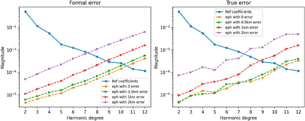
Figure 10. Power spectra in Case 3 listed in Table 3 (Different Deimos ephemeris errors).

The sunlight radiation impinging on the surface of the spacecraft exerts pressure, thereby influencing its orbit. In this study, a simplified approach was employed, treating the spacecraft as spherical and assuming that the sunlight rays are always perpendicular to the spacecraft surface for modeling solar radiation pressure. The simplified equation for calculating solar radiation pressure is shown in Eq. 9:

$a_{SRP}=-C_r{P}_s\frac{A}{m}\frac{r}{\left|r^3\right|}a{u}^2(9)$

where $C_r$ is the SRP coefficient, primarily determined by the spacecraft’s surface material, typically treated as an estimated parameter in precise orbit determination, $r$ represents the position vector of the Sun relative to the spacecraft, $P_s$ denotes the solar radiation pressure per unit area at a distance $\left|r\right|$, typically taken as 4.56 × 10⁻⁶ N m⁻², $A$ and $m$ are the surface area and mass of the spacecraft.

It is necessary to note that the spacecraft is not always fully exposed to solar radiation, and shadowing due to celestial bodies needs to be considered. In such cases, Formula 7 should be multiplied by a shadowing coefficient $v$.

In this study, the numerical value of Cr was set to 1.2. In comparative experiments, errors of 0%, 10%, 20%, and 30% were respectively added to the Cr values to investigate the impact of Cr errors on the calculation results. Figure 11 illustrates the power spectra of the calculation results with the aforementioned errors added to Cr.

Figure 11

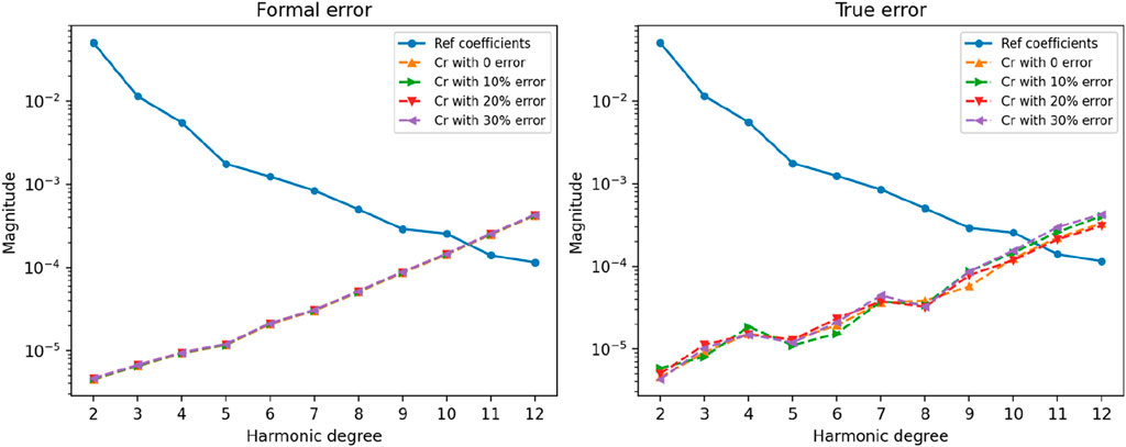
Figure 11. Power spectra in Case 4 listed in Table 3 (Different Cr errors).

As shown in Figure 11, the addition of Cr errors has a relatively small impact on the variance of the true error of the gravitational field coefficients, and it hardly affects the formal error. In the orbiting scenario, the perturbation force provided by solar radiation pressure is much smaller and relatively stable compared to that provided by Mars and Deimos.

4 Discussion and conclusion

This paper addresses gravity field recovery at Deimos under multiple exploration scenarios, with a focus on Martian moon exploration missions. Based on simulated ground tracking data, the paper conducts precise orbit determination of spacecraft with close orbit around Deimos and inversely estimates the gravity field model of Deimos. The main work and innovations of this paper are summarized as follows.

Based on the available low-order gravity field coefficients of Deimos and rescaled gravity field coefficients of Phobos, we constructed of a 20th-degree gravity field model of Deimos, and the Kaula criterion was applied for validation and adjustment. Simulated analyses were conducted separately in the flyby and orbiting scenarios around Deimos, establishing force models and observation models for spacecraft. Then we analyzed and evaluated the calculated results to determine the effective degrees for inversion of the Deimos gravity field. Factors affecting the accuracy of the calculation and their respective influences were studied and analyzed through comparative experiments. From the experiment results of this study, it is evident that, based on the current technological capabilities, the altitude of the spacecraft relative to Deimos has the greatest impact on the accuracy of the calculations. Under the influence of Martian perturbations, increasing the spacecraft’s altitude leads to a sharp decrease in the accuracy of the calculations and the feasible degree of gravity field coefficients. Then, the level of noise in the observation data and the errors in Deimos’ ephemeris play significant roles, but the former can be addressed through improvements in observation methods and equipment, while the latter can be constrained by precise orbit determination of Deimos. Conversely, errors in the solar radiation pressure coefficient have a relatively minor impact on the calculation results. Furthermore, this paper compared the calculated GM with existing findings, indicating that a targeted mission would significantly reduce error bars of GM. Additionally, various parameter evaluation criteria were employed to demonstrate the reliability of the results obtained in this study.

This study utilized simulated data, and the orbit state around Deimos were conducted at relatively close distances. Moreover, in the processing of actual radio tracking data, besides minor effects from modeling factors like solar radiation pressure, there are significant long-term impacts from errors in rotation models and celestial ephemerides (Liu et al., 2023). Due to the simplifications made during the simulation, the results of the study may be somewhat idealized. However, the experimental process and data processing methods still hold relevant reference value. In future real data processing endeavors, finer adjustments or modeling efforts will be planned to achieve high precision outcomes.

The gravity field of Deimos is of significant importance for scientific research and deep space exploration within the Martian system. The computational results presented in this paper can serve as a priori gravity field models for Martian moon exploration missions, providing theoretical foundations for spacecraft navigation and landing orbit determination. Additionally, they offer valuable insights for the planning and implementation of future exploration missions to Mars and its satellites by various countries.

Data availability statement

The raw data supporting the conclusions of this article will be made available by the authors, without undue reservation.

Author contributions

WS: Data curation, Formal Analysis, Software, Writing–original draft. JY: Conceptualization, Funding acquisition, Supervision, Writing–review and editing. SS: Software, Writing–review and editing. YY: Validation, Writing–review and editing. SL: Validation, Writing–review and editing. ZW: Supervision, Visualization, Writing–review and editing. J-PB: Supervision, Writing–review and editing.

Funding

The author(s) declare that financial support was received for the research, authorship, and/or publication of this article. This work is supported by the National Key Research and Development Program of China (No. 2022YFF0503202) and the National Natural Science Foundation of China (42241116). JY is supported by the Macau Science and Technology Development Fund [No. SKL-LPS(MUST)-2021-2023] and the 2022 Project of Xinjiang Uygur Autonomous Region of China for Heaven Lake Talent Program; ZW is supported by the Chinese Academy of Sciences Foundation of the young scholars of western (2020-XBQNXZ-019) and the open project of the Key Laboratory in Xinjiang Uygur Autonomous Region of China (2023D04058); and J-PB is supported by a DAR grant in planetology from the French Space Agency (CNES).

Acknowledgments

We sincerely appreciate the reviewers and the editor for their constructive comments, which greatly improved our submission manuscript.

Conflict of interest

The authors declare that the research was conducted in the absence of any commercial or financial relationships that could be construed as a potential conflict of interest.

Publisher’s note

All claims expressed in this article are solely those of the authors and do not necessarily represent those of their affiliated organizations, or those of the publisher, the editors and the reviewers. Any product that may be evaluated in this article, or claim that may be made by its manufacturer, is not guaranteed or endorsed by the publisher.

References

Archinal, B. A., Acton, C. H., A’Hearn, M. F., Conrad, A., Consolmagno, G. J., Duxbury, T., et al. (2018). Report of the IAU working group on cartographic coordinates and rotational elements: 2015. Celest. Mech. Dyn. Astr. 130, 22. doi:10.1007/s10569-017-9805-5

CrossRef Full Text | Google Scholar

Cutts, J. A. (1974). Mariner Mars 1971 television picture catalog. volume1: experiment design and picture data, NASA-CR-140700 [R]. Pasadena: NASA.

Google Scholar

Desprats, W., Arnold, D., Blanc, M., Jäggi, A., Li, M., Li, L., et al. (2021). Recoverability of Callisto gravity field influenced by orbiter mission characteristics. EGU General Assem., EGU21–9959. online, 19–30 Apr 2021. doi:10.5194/egusphere-egu21-9959

CrossRef Full Text | Google Scholar

Dunbar, B. (2009). Mars' moon Deimos [OL]. NASA. 2017-08-07)[2021-6-1]. Available at: https://www.nasa.gov/multimedia/imagegallery/image_feature_1302.html.

Google Scholar

Gao, W., Yan, J., Jin, W., Yang, X., Yang, C., Ye, M., et al. (2021a). A simulation experiment on the GM estimation for Comet 133P/Elst-Pizarro. Res. Astronomy Astrophysics 21 (1), 016. doi:10.1088/1674-4527/21/1/16

CrossRef Full Text | Google Scholar

Gao, W., Yan, J., Wang, B., Xi, G., Ye, M., Jin, W., et al. (2021b). A lander radio science experiment for the estimation of the gravity field and rotation of comet 133P/Elst-Pizarro. Mon. Notices R. Astronomical Soc. 505 (1), 103–115. doi:10.1093/mnras/stab1297

CrossRef Full Text | Google Scholar

Gao, W., Yan, J., Wang, B., Yang, W., Li, F., and Jean-Pierre, B. (2023). A three-degree and ordered gravity model of the comet67P/Churyumov-Gerasimenko based on an improvedcomet ephemeris. Sci. Sinica Phys. Mech. Astronomica 53, 259513. doi:10.1360/sspma-2022-0420

CrossRef Full Text | Google Scholar

Genova, A., Goossens, S., Lemoine, F. G., Mazarico, E., Neumann, G. A., Smith, D. E., et al. (2016). Seasonal and static gravity field of Mars from MGS, Mars odyssey and MRO radio science. Icarus 272, 228–245. doi:10.1016/j.icarus.2016.02.050

CrossRef Full Text | Google Scholar

Guo, X., Yan, J., Yang, X., and Jean-Pierre, B. (2020). High degree phobos gravity field modeling based on shape model. Geomatics Inf. Sci. Wuhan Univ. 45 (4), 604–611. doi:10.13203/j.whugis20190104

CrossRef Full Text | Google Scholar

Heiskanen, W. A., and Moritz, H. (1976). Physical geodesy. Bull. Géodésique 86 (1), 491–492. (1946-1975). doi:10.1007/bf02525647

CrossRef Full Text | Google Scholar

Jacobson, R. A. (2010). The orbits and masses of the Martian satellites and the libration of Phobos. Astronomical J. 139 (2), 668–679. doi:10.1088/0004-6256/139/2/668

CrossRef Full Text | Google Scholar

Kaula, W. M., and Street, R. E. (1967). Theory of satellite geodesy: applications of satellites to geodesy. Phys. Today 20 (10), 101. doi:10.1063/1.3033941

CrossRef Full Text | Google Scholar

Konopliv, A. S., Park, R. S., and Folkner, W. M. (2016). An improved JPL Mars gravity field and orientation from Mars orbiter and lander tracking data. Icarus 274, 253–260. doi:10.1016/j.icarus.2016.02.052

CrossRef Full Text | Google Scholar

Konopliv, A. S., Yoder, C. F., Standish, E. M., Yuan, D., and Sjogren, W. L. (2006). A global solution for the Mars static and seasonal gravity, Mars orientation, Phobos and Deimos masses, and Mars ephemeris. Icarus 182, 23–50. doi:10.1016/j.icarus.2005.12.025

CrossRef Full Text | Google Scholar

Kuramoto, K., Kawakatsu, Y., Fujimoto, M., Genda, H., Imamura, T., Kameda, S., et al. (2018). Martian moons exploration(MMX) conceptual study update[C]. 49th lunar and planetary science conference. Woodlands, 214.

Google Scholar

Lee, P. (2016). Third international conference on the exploration of Phobos and Deimos [OL]. Moffet field. NASA Ames Research Center. Available at: https://phobos-deimos.arc.nasa.gov/.

Google Scholar

Liu, S. (2022). Scientific applications of radio tracking data from deep space probes. Geomatics Inf. Sci. Wuhan Univ. (002), 047. doi:10.13203/j.whugis20210685

CrossRef Full Text | Google Scholar

Liu, S., Yan, J., Yang, X., Ye, M., Guo, X., Wang, B., et al. (2023). Potential contribution of tianwen-1 extended mission to Mars low-order gravity field. Geomatics Inf. Sci. Wuhan Univ. 48 (1), 58–64. doi:10.13203/j.whugis20210035

CrossRef Full Text | Google Scholar

Mathews, P. M., Dehant, V., and Gipson, J. M. (1997). Tidal station displacements. J. Geophys. Res. Solid Earth 102 (B9), 20469–20477. doi:10.1029/97jb01515

CrossRef Full Text | Google Scholar

Montenbruck, O., and Gill, E. (2012). Satellite orbits: models, methods and applications. Berlin: Springer Science & Business Media.

Google Scholar

Nakamura, T., Ikeda, H., Kouyama, T., Nakagawa, H., Kusano, H., Senshu, H., et al. (2021). Science operation plan of Phobos and Deimos from the MMX spacecraft. Earth Planets Space 73, 227. doi:10.1186/s40623-021-01546-6

CrossRef Full Text | Google Scholar

Rubincam, D. P., Benjamin, F. C., and Thomas, P. C. (1995). The gravitational field of Deimos. Icarus 114 (1), 63–67. ISSN 0019-1035. doi:10.1006/icar.1995.1043

CrossRef Full Text | Google Scholar

Sagdeev, R. Z., and Zakharov, A. V. (1989). Brief history of the phobos mission. Nature 341, 581–585. doi:10.1038/341581a0

CrossRef Full Text | Google Scholar

Smith, D. E., LeMoine, F., and Zuber, M. T. (1995). Simultaneous estimation of the masses of Mars, Phobos, and Deimos using spacecraft distant encounters. Geophys. Res. Lett. 22, 2171–2174. doi:10.1029/95gl01801

CrossRef Full Text | Google Scholar

Sun, S., Yan, J., Gao, W.-T., Wang, B., Wang, Z., Ye, M., et al. (2023). Simulated gravity field estimation for the main belt comet 133P/Elst-Pizarro based on a satellite-to-satellite tracking mode. Res. Astronomy Astrophysics 23 (9), 095012. doi:10.1088/1674-4527/acdc89

CrossRef Full Text | Google Scholar

Tieying, Li, Zheng, G., and Xiao, Z. (2021). Survey of space observations and research on topography and geomorphology of Deimos. Chin. Space Sci. Technol. 41 (05), 1–9. doi:10.16708/j.cnki.1000-758X.2021.0061

CrossRef Full Text | Google Scholar

Williams, D., and Friedlander, J. (2015). Deimos-Viking2 orbiter (30km)[OL]. NASA, 2015(2015-09-24)[2024-03-01]. Available at: https://nssdc.gsfc.nasa.gov/imgcat/html/object_page/vo2_423b63.html.

Google Scholar

Witasse, O., Duxbury, T., Chicarro, A., Altobelli, N., Andert, T., Aronica, A., et al. (2014). Mars express investigations of phobos and Deimos. Planet. Space Sci. 102 (11), 18–34. doi:10.1016/j.pss.2013.08.002

CrossRef Full Text | Google Scholar

Yang, X., Yan, J., Liu, S., Ye, M., Jin, W., Li, F., et al. (2019). Low-degree gravity field recovery of Phobos based on MEX flyby data. Sci. Sinica Phys. Mech. Astronomica 49 (05), 105–114.

CrossRef Full Text | Google Scholar

Yamamoto, K., Matsumoto, K., Ikeda, H., Senshu, H., Willner, K., Ziese, R., et al. (2023). Simulation of gravity field estimation of Phobos for Martian Moon eXploration (MMX). Res. Square. doi:10.1186/s40623-024-02017-4

CrossRef Full Text | Google Scholar

Yang, X. (2023). Mars spacecraft precise orbit determination and phobos gravity field recovery. Acta Geod. Cartogr. Sinica 52 (06), 1043. doi:10.11947/j.AGCS.2023.20210692

CrossRef Full Text | Google Scholar

Appendix

As shown in Table A1, in the Appendix, we give the reference gravity field model of Deimos that is generated from the shape model. The gravity field model of Deimos is given up to degree and order of 4.

TABLE A1

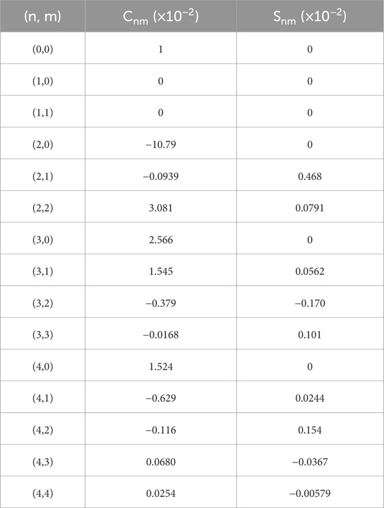
TABLE A1. The reference gravity field model of Deimos.