- 1Astrophysics Department, Argelander Institut für Astronomie, University of Bonn, Bonn, Germany
- 2Space Weather Laboratory, NASA Goddard Space Flight Center, Greenbelt, MD, United States
- 3Department of Physics, Catholic University of America, Washington DC, United States
- 4Department of Electrical and Computer Engineering, University of Illinois at Urbana-Champaign, Urbana, IL, United States
Remote sensing observations of far-ultraviolet (FUV) emissions have been used to estimate 3D neutral hydrogen (H) density models of the terrestrial exosphere under solar minimum (2008) and solar maximum (2013 and 2015) conditions. Specifically, we used Lyman-alpha (Lyman-
1 Introduction
The exosphere is the uppermost layer of the terrestrial atmosphere that extends from ∼500 km (its inner boundary, known as the exobase) up to Earth radii of ∼60 (Re; 1 Re = 6,371 km) (Baliukin et al., 2019). This region is mainly populated with atomic neutral hydrogen (H), which resonantly scatters solar Lyman-alpha (Lyman-
Several efforts to estimate H density from far-ultraviolet (FUV) observations have been thoroughly conducted in the last four decades. For example, Rairden et al. (1986) generated an H-density profile utilizing Lyman-
Since June 2008, NASA’s Two Wide-angle Imaging Neutral-atom Spectrometers (TWINS) mission, which includes two satellites TWINS1 and TWINS2, has been acquiring routine measurements of geocoronal H Lyman-
TWINS/LAD radiance data have been used to estimate 3D H-density models using more sophisticated inversion methods. Zoennchen et al. (2015) used a parametric fitting approach to a spherical harmonics function of order 2 to estimate a set of exospheric density models. Data acquired in June 2008 and June 2010 during quiet geomagnetic conditions were used to generate a solar minimum model. Similarly, data acquired from October to December 2012 were used to generate a model for solar maximum conditions. This study reported, for the first time, the response of the exospheric density and structure to the solar cycle. More recently, Cucho-Padin and Waldrop (2018) implemented a high degree-of-freedom (DOF) tomography approach, which allows the estimation of density distributions without the dependence on ad hoc functions, allowing the identification of intricate spatial structures. Data for a single day in 2008 (solar minimum) were used to demonstrate the feasibility of this technique. Radial H-density profiles of the outer exosphere, in particular close to the subsolar point (SSP) derived from Lyman-α observations, are discussed by Cucho-Padin et al. (2022) and Zoennchen et al. (2022). Furthermore, H-density values at 10 Re near the subsolar point derived from different observations from Lyman-α are also discussed [i.e., with XMM-Newton X-ray by Connor and Carter (2019) or with IBEX-ENA/MMS by Fuselier et al. (2020)].
In this article, we implement three models of the H exosphere using TWINS LAD data acquired during solar minimum (2008) and solar maximum conditions (2013 and 2015) to investigate the response of the density distributions to a solar cycle. Each dataset is formed using several days of data to provide an appropriate coverage of the exospheric region. We process data from each year independently and introduce a self-consistent handling of two different Lyman-
2 Materials and methods
2.1 Approach and LOS corrections
Under the assumption of single scattering in the optically thin regime, the local exospheric density
with
where 1,050 K is an exospheric reference temperature derived by Rairden et al. (1986).
The solar Lyman-α line-center flux can be calculated from the total solar Lyman-α flux (which is provided by SEE/TIMED) using the relation given by Emerich et al. (2005).
In addition to the exospheric contribution, every measurement contains a background from the Lyman-α glow of the interplanetary H atoms (IPH background), which needs to be subtracted. Here, we used a hot model of the interplanetary H-density distribution (Fahr, 1971; Thomas, 1978). Based on that model, we calculated daily all-sky maps of the Lyman-α flux from the IPH background. The model parameters and assumptions used are widely described by Zoennchen et al. (2015).
The Earth albedo correction term
First is the backscattered Lyman-α re-emission from lower (optically thick) exospheric shells with high H densities at the dayside (acts as a secondary source of Lyman-α). This secondary dayside Lyman-α radiation was modeled using a Monte Carlo (MC) model based on the solar minimum 3D H-density distribution proposed by Zoennchen et al. (2015). The largest enhancement of the local g-factor due to this effect is located at the dayside (near the subsolar point) at low distances. At our lower model boundary at 3.75 Re, the local g-factor is enhanced by ∼15%. The dayside enhancement decreases rapidly with increasing radial distance. The influence of H-density variations during the solar cycle on the local g-factor enhancement is expected to be very small. One reason is the expected low variance of the H-density level with the solar cycle at low distances near the exobase (Chamberlain, 1963), where most of Earth’s albedo Lyman-α emissions originate from. Therefore, in this work, we used the same modeled local g-factor enhancement due to albedo emission for all inversions.
Second is the self-absorption term of the solar Lyman-α flux when it enters the exosphere at the dayside (i.e., at 10 Re) and transits toward the nightside (see blue arrow in Figure 1). This correction term was implemented self-consistently in the model fitting process by considering the optical depth
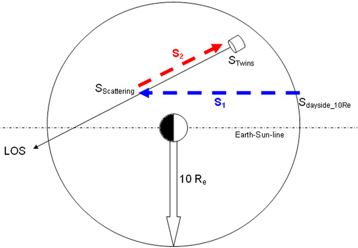
Figure 1. Two corrections (blue and red arrows) for geocoronal Lyman-α absorption at an integration LOS-position SScattering: (1) blue arrow: absorption due to the optical depth between SScattering and Sdayside_10Re (dimming of solar Lyman-α flux penetrating the exosphere); (2) red arrow: loss of scattered exospheric Lyman-α photons to the detector due to the optical depth between SScattering and STwins.
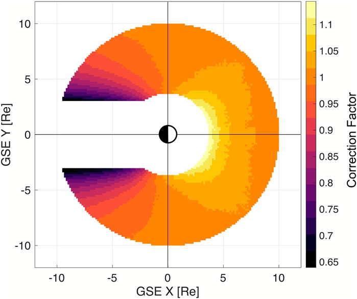
Figure 2. Ecliptic map (in GSE coordinates) of the combined effect of secondary Lyman-α from Earth re-emission (mostly at the Earth dayside) and exospheric self-absorption of solar Lyman-α radiation (mostly on the Earth nightside). This map is based on the H-density distribution from the solar minimum SHR model inversion (2008).
Additionally, our emission model includes a third correction term,
The local cross section σ needed for the calculation of optical depths τ1 and τ2 is a function of the local exospheric temperature Texo (see Equation 2). As an approximation of the local Texo, we used a relation from COSPAR. Working Group IV (1965), where it is a function of the solar activity level (solar F10.7 cm radio flux) and the Geocentric Solar Ecliptic (GSE) longitude. Note that there is a relation between solar F10.7 cm radio flux and total solar Lyman-α flux (Vidal-Madjar, 1975). Figure 3 shows the GSE-longitudinal Texo values used in this work for our data selections of solar minimum and maximum to calculate the local cross section σ.
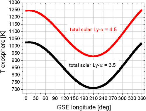
Figure 3. Longitudinal variation in the exospheric temperature [K] for the total solar Lyman-α fluxes 3.5 (black—solar minimum) and 4.5 (red—solar maximum) based on temperature profiles from COSPAR. Working Group IV (1965).
2.2 Reconstruction of the exospheric 3D H-density distribution
For the reconstruction of the exospheric 3D H-density distribution, we applied two independent tomographic inversion methods as described in the following subsections. The expression “tomographic inversion” refers to a method that retrieves a local 3D distribution from a sample of (intersecting) multipositional and multidirectional line-of-sight integrated observations.
2.2.1 Method A: 3D inversion based on an SHR model
SHRs are widely used as a functional base to reconstruct the exospheric H-density distribution [(Hodges, 1994) with a polynomial number L = 3 (Nass et al., 2006; Zoennchen et al., 2015; Bailey and Gruntman, 2011) and L = 2].
To calculate the modeled LOS column brightness, we used the exospheric H-density model proposed by Zoennchen et al. (2015) with improvements in two aspects.
First, the radial power law function was enhanced by an additional term since it better fits the radial behavior of the column brightness data compared to a pure power law. Second, the polynomial number of the SHR was increased from L = 2 to 3 in order to capture spatial variations having higher angular frequencies.
Here,
To take into account that the maximal impact distance (at the Earth tangent point) of the available LOSs is approximately 6 Re, we limited the radial variation of
With a least squares fit procedure, the difference between observed and modeled LOS column brightness can be minimized:
Since the observational global coverage of the exosphere by TWINS LAD is incomplete, this fit function is expanded by a regularization term c, described below, to enforce a solution with optimal angular smoothness:
An inversion of TWINS Lyman-α data with the additional use of 3D regularization was first introduced by Cucho-Padin and Waldrop (2018). Since our inversion is based on a parametric density model with an r-dependence constraint in terms of an approximate power law, we only need to regularize the two angular dimensions (2D). The regularization term
Factor λ scales the strength of the angular smoothness against the
For the “training” subset, we used TWINS1 LAD1 and TWINS2 LAD2 data of 12 June 2008. The “testing” subset contained TWINS1 LAD2 and TWINS2 LAD1 data of the same day. Using these subsets, we found the optimal model predictability with λ = 2.01. This value for λ was also used for the density inversion from the data of 2013 and 2015 (for the description of the LAD data selections, see Section 2.3).
2.2.2 Method B: 3D inversion based on the “high-DOF” method
In order to validate the parametric estimations of 3D H-density distributions, we also utilized a parametric-free approach to reconstruct exospheric density from TWINS radiance data. In contrast to parametric estimation, this possesses a high DOF to reproduce intricate spatial structures in the H density. This method is thoroughly described by Cucho-Padin et al. (2022) and is briefly summarized here. First, we adopted a spherical solution domain that includes only the optically thin region (valid zone for Equation 1). This sphere has an inner and outer radius equal to 3 and 25 Re, respectively. Second, we discretized the solution domain into uniform spherical voxels with dimensions ∆r = 0.25 Re and ∆ϕ = ∆θ =
In this study, we generated
where
To generate the covariance matrix of measurements,
To generate the “precision matrix”
In this methodology, we also included the correction for geocoronal Lyman-α absorption, as well as the correction for Earth’s albedo. To do so, we first estimated the H-density distributions with no corrections and used the new
2.3 Selections of TWINS LAD data
As a representation of the solar minimum near the summer solstice, our first selection contains LAD observations of TWINS1 and 2 from 12 June 2008. This day corresponds to quiet solar conditions, 3 days before a geomagnetic storm onset. On this day, the apogees of TWINS1 and 2 are situated longitudinally (GSE) on the dawn and dusk side at an angle of ∼20° from the noon–midnight meridian. This viewing geometry enables stereoscopic coverage of the dayside H-geocorona. For the solar maximum dataset, we used near-summer solstice TWINS1 LAD observations from 2013 to 2015. We created two separate selections with quiet-time data (with Dst-indexes near 0) from 2013 (23 July and 12 August) and 2015 (04 June, 03 July, and 19 July). These selections involve LAD data from multiple days in order to obtain a stereoscopic view, which is comparable to the viewing geometry in the 2008 data selection described above. As a result, the solar minimum and maximum data selections are very comparable in terms of angular viewing geometry, season, and geomagnetic activity.
We restricted the data to LOSs having geocentric impact distances ≥3.75 Re. Beyond this distance, the relevant scattering processes correspond to an optically thin regime. All observations with LOS-Sun angles ≤90° are omitted from the data because they are contaminated by scattered sunlight. LOSs with tangent point radial distances ≤3 Re are also excluded from the negative GSE x-axis (nightside) to avoid LOSs that cross regions near the shadow of Earth’s penumbra. Lastly, all LOSs crossing the 8° angular region around one of the tracked UV-bright stars [list of stars taken from the study by Snow et al. (2013)] are removed.
2.4 Solar and geomagnetic conditions
The data selection of 12 June 2008 represents the H-geocorona on a quiet day near the summer solstice in solar minimum. The solar total Lyman-α flux is very low at 3.54 [
The other two data selections used here, from mid-2013 and mid-2015, represent the H-geocorona in the same season but during solar maximum conditions. The selected days can also be considered geomagnetic quiet with daily averaged Dst indexes near 0 [nT], which rules out the direct onset of a geomagnetic storm. Nevertheless, the total solar Lyman-α flux is significantly higher, with averaged values of 4.47 (2013) and 4.53 (2015) [
2.5 LAD sensitivity calibration
The TWINS LAD detectors observed exospheric Lyman-α column brightness (in [counts/s]) along LOSs with a field of view of approximately 4°. The observed count rates were converted into the physical unit Rayleigh [R]. This was done using the LAD sensitivity factors
The calibration procedure presented here is customized for this study. To the best of our knowledge, no citable standard TWINS LAD calibration and no high data levels are available at this time. Nevertheless, the stellar peak levels, together with the related LAD sensitivity factors found in this work, might be useful for the community as standards of the analyzed periods.
The LAD sensitivity values from the data selections for 2013 and 2015 deviate significantly from their initial values in 2008, which motivates the recalibration conducted for this study. The TWINS LAD sensitivity
For the TWINS1 LAD2 data from 2015, we used the initial Lyman-α peak flux of June 2008 of the star Spica and compared it directly to the peak value measured from observations in mid-2015 (see Figure 4, upper row). A depletion in the TWINS1 LAD2 sensitivity by a factor of about 0.35 was derived. Regarding the TWINS1 LAD2 data from 2013, an additional cross-calibration step of Spica with the second star β Cen (galactic long/lat: 311.7°/1.25°) in mid-2010 was necessary since Spica was not observed by LAD2 on the days of our 2013 selection (see Figure 4, lower row). For validation, the stars α Cru and λ Sco were also used.
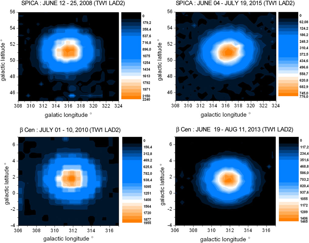
Figure 4. Cross-calibration of TWINS1 LAD2 for mid-2015 and 2013 (upper row: June 2008 versus June–July 2015 using observations of star Spica; lower row: July 2010 versus June–August 2013 using observations from star β Cen).
Furthermore, the sensitivities of both LADs of TWINS2 (as used in the 2008 data selection) are recalibrated against the LADs of TWINS1 (see Figure 5) using the stars σ Sgr and α Cru. All sensitivity factors used in this work are listed in Table 1.
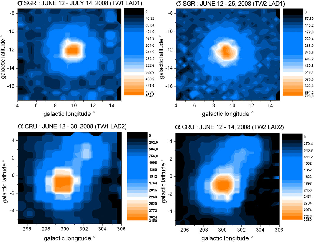
Figure 5. Lyman-α detector cross-calibration of TWINS2 against TWINS1 in 2008 (upper row: TWINS1 LAD1 versus TWINS2 LAD1 using LAD observations of star σ Sgr in June/July 2008; lower row: TWINS1 LAD2 versus TWINS2 LAD2 using LAD observations of star α Cru in June 2008).
An estimate of the calibration uncertainty is needed to evaluate the H-density variation between solar minimum (2008) and maximum (2013, 2015) found in this work. As shown in Table 1, for TWINS1 in 2015, the sensitivities of both LADs experienced a heavy decrease (LAD1 to ∼1/7 and LAD2 to ∼1/3) with respect to their initial values. In 2013, the decrease was not that strong but was also significant (LAD1 to ∼1/3 and LAD2 to ∼1/2). Besides the noise-to-peak ratio of the reconstructed stellar images, there is uncertainty due to the intrinsic stellar UV-flux variation over the considered time period. Both effects can be quantified (in sum) by analyzing the standard deviation of the individual peak-level decreases of multiple stars. As shown in Table 2, the values for the relative peak-level decrease derived from different stars for the same period/same LAD are quantitatively very close together. This speaks for a good noise-to-peak ratio in the images and for stable stellar UV-fluxes of the used stars. For TWINS1, it was found that the LAD2 calibration based on α Cru and λ Sco has 4.6% (2013) and 4.2% (2015) uncertainty with respect to the Spica-based value, respectively. The LAD1 calibration uncertainties are 3.2% (2013) and 6.2% (2015). From these values, we assume an averaged calibration uncertainty of ∼5% for both LADs and both solar max years.
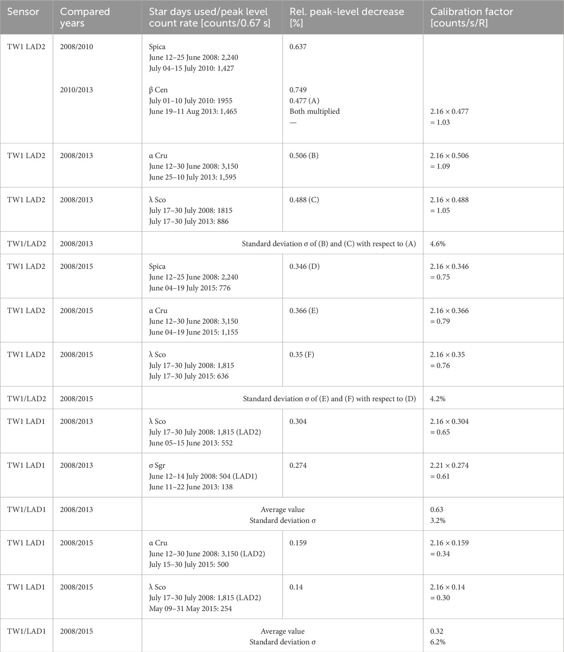
Table 2. Lyman-α peak-level count rates of different UV-bright stars measured with the two LADs of TWINS1 near summer 2008, 2013, and 2015. The reduction in the LAD-sensitivity between 2 years is equivalent to the reduction in the peak-level count rates of a given star during the same time. By comparing the peak-level reductions of multiple stars over a period (observed by the same LAD), the uncertainty of this calibration method was found to be 3%–6% (on average, ∼5%).
3 Results
3.1 Normalized radial Lyman-α profiles at solar minimum and maximum
Figure 6 shows the normalized radial profiles of the measured exospheric Lyman-α column brightness between 3.75 and 6.0 Re (LOS impact distance) for solar minimum and maximum (IPH background and the effect of the scattering phase function are removed). Here, normalized means that the effect of a brighter solar Lyman-α illumination at solar maximum than at solar minimum is removed by normalizing the solar maximum profiles to the lower scattering rate of the total solar Lyman-α flux at solar minimum. As shown in Figure 6, the solar maximum profiles (2013 and 2015) both show significantly higher Lyman-α column brightness values than the solar minimum profile. Since the effect of a brighter solar illumination is removed, the remaining higher values at solar maximum reflect larger hydrogen column densities than those at solar minimum. This result is evident directly from the column brightness profiles shown in Figure 6.
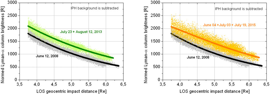
Figure 6. TWINS LAD Lyman-α column brightness profiles observed at spacecraft distances ≥6.5 Re (LOSs impacting the bright dayside nose within an angular distance <75° from the subsolar point are excluded from these plots).
A correct calibration of the LAD sensitivity between the years of solar minimum (2008) and maximum (2013 and 2015) is essential when comparing exospheric H-density levels. The relative uncertainty of the calibration method used in this work, which, based on the peak values of multiple UV-bright stars, was found to be, on average, ∼5%. This is significantly smaller than the enhancement of the Lyman-α column brightness profile at solar maximum compared to minimum (as shown in Figure 6).
3.2 Comparison of the 3D H-density distributions
Figure 7 shows the 3D H-density distributions for solar minimum (2008) and maximum (2013 and 2015) derived from the two independent 3D inversion techniques described in Section 2.2.1 (with the SHR formulation) and Section 2.2.2 (“high degree-of-freedom” method). The results from both inversion techniques are very similar in terms of angular distribution and total exospheric H density at the lower and upper boundary of 3.75 and 6.0 Re, respectively. Since the angular resolution of the SHR method is limited by its polynomial order (=3), the H-density distributions from the HDOF method show slightly more structures than the SHR results. The numerical values for the SHR model coefficients are listed in Table 3.
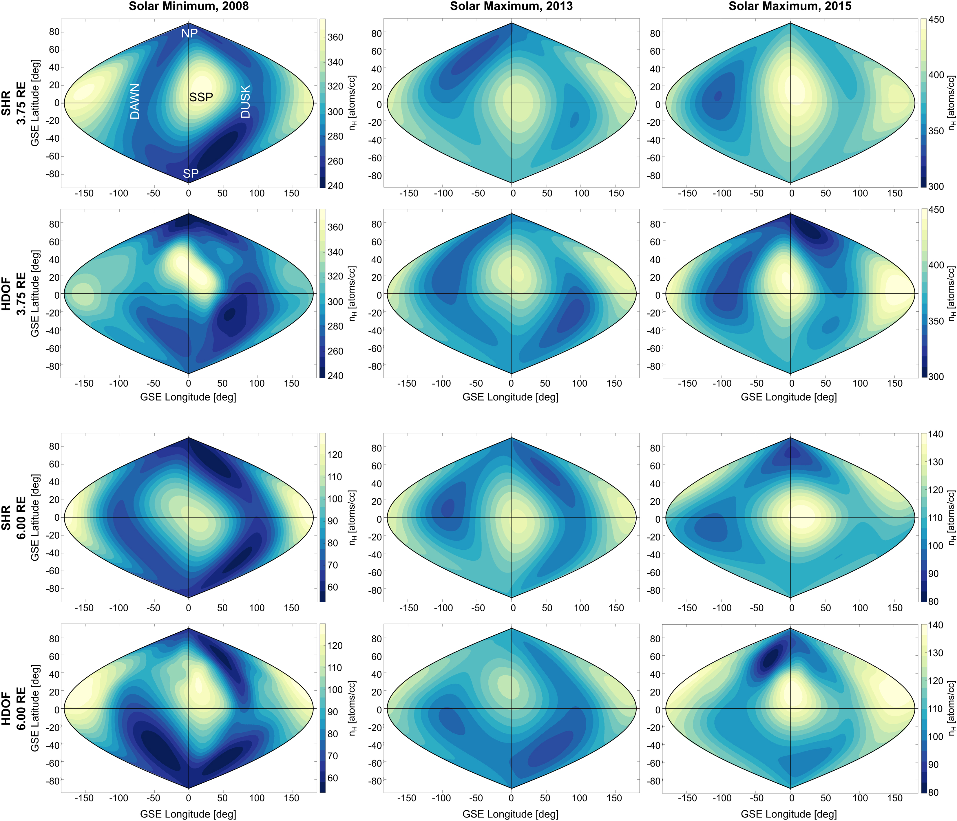
Figure 7. H-density distributions estimated from both inversion methods: SHR model (see section 2.2.1) and HDOF technique (see section 2.2.2). The first and second rows show estimated H-density distributions at a geocentric distance of 3.75 Re using the SHR model and HDOF technique, respectively. Tomographic estimations used data on near summer solstice for 2008 (left column), 2013 (middle column), and 2015 (right column). The third and fourth rows show H densities at 6.00 Re using the SHR model and HDOF technique, respectively. Most significant regions of enhanced H density are at the dayside (“nose”) near the subsolar point at GSE longitude/latitude ∼15°/10° and at the nightside (“tail”) near midnight. Density enhancements near the nose and tail are visible in the inversions for both solar minimum and maximum. Both the absolute H density and its angular distribution (nose and tail features) are very similar to the results found with the SHR model inversion. NP, North ecliptic pole; SP, South ecliptic pole.
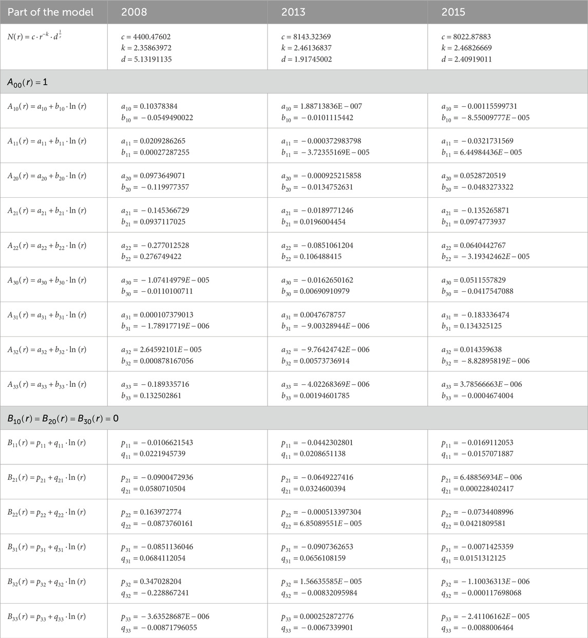
Table 3. Model fit coefficients for the spherical harmonic models of the 3D hydrogen density distribution at solar minimum (2008) and solar maximum (2013 and 2015).
The exosphere over this distance range clearly deviates from a radial symmetric distribution. Most significant is a strongly enhanced region on the dayside near the SSP. This dayside “nose” is visible in all inversions and provides an H-density peak value that is 20%–50% larger than the H densities of the surrounding “off-nose” angular regions on the same radial shell. A second region of enhanced H densities is present on the nightside near midnight. This “tail” structure also appears in all inversions with a varying level of significance.
The integrated (over 1° × 1° angular segments) number of H-atoms within 3.75–6.0 Re is shown in Figure 8 separately for both inversion methods. The described “nose” and “tail” regions of enhanced H densities appear in these images with their highest significance and contrast. To identify angular regions with the largest solar cycle-dependent H-density enhancement, the ratio of solar maximum to minimum of the integrated H-atom number density at every angular segment was calculated. The result is plotted for both inversion techniques in Figure 9 (left image: SHR model; right image: “high degree-of-freedom” method). The most significant relative H-density enhancements are at the dayside (mostly at mid-to-high latitudes), with a preference for the dusk side. It is noteworthy that the enhancement close to the dayside nose (near the SSP) appears to be relatively low.
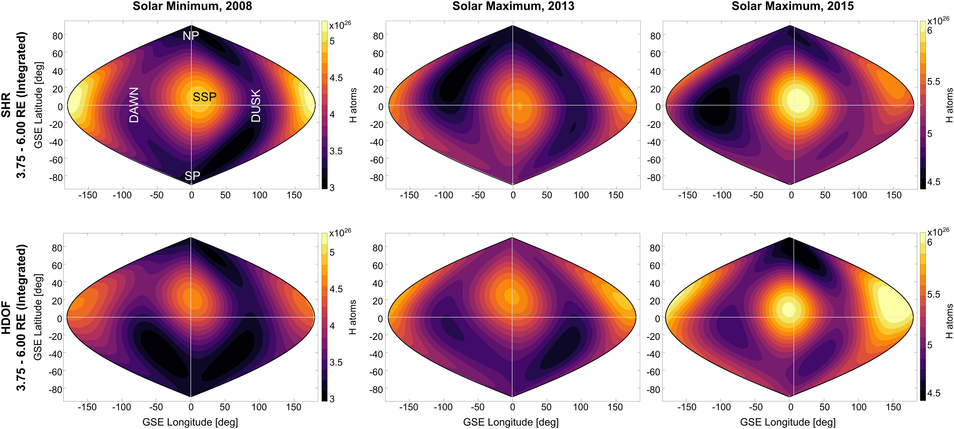
Figure 8. Total number of neutral exospheric H-atoms between 3.75 and 6.00 Re near the summer solstice for 2008 (left), 2013 (middle), and 2015 (right). The first row shows the total H content in the 3.75–6.00 Re region derived from the tomographic estimations using the SHR model. Similarly, the second row shows results using the HDOF technique. Dayside nose and nightside tail structures are present in all reconstructions during solar minimum and solar maximum conditions.

Figure 9. Angular view of the relative solar cycle enhancement of H density integrated between 3.75 and 6 Re (left: based on the SHR model; right: based on the “high degree-of-freedom” method). Plotted is the ratio of the H-atom number density (integrated from 3.75 to 6.0 Re near the summer solstice) at solar maximum (2013 and 2015 averaged) relative to solar minimum (2008). The most significant relative H-density enhancements are visible at mid-to-high latitudes with a preference for the dusk side. Surprisingly, the enhancement close around the dayside nose (near the SSP) appears to be relatively low.
The total number of H-atoms within 3.75–6.0 Re, calculated as the sum of H-atoms within all 1° × 1° angular segments, is approximately 35% larger at solar maximum than at solar minimum [based on the SHR model: 33% (2013) and 36% (2015); based on the “high degree-of-freedom” method: 35% (2013) and 37% (2015)].
A major result of this work is that within 3.75–6.0 Re, the solar maximum H density is larger than that of solar minimum at the same geocentric distance r0 and angular position. This finding can be interpreted as a more expanded exosphere during solar maximum. To quantify the amount of radial expansion, we calculated the geocentric distance, rexp, where the H density at solar maximum equals the solar minimum H density at r0. The amount of radial expansion can then be defined as
Furthermore, to analyze quantitatively the difference in exospheric H content between solar maximum and minimum conditions, we implemented histograms of integrated H-atoms from radial shells at 3.75–6 Re for both inversion techniques, which are shown in Figure 10 (note that the data have been taken from Figure 8). For solar minimum conditions, integrated H-atoms range from 3 to 5 × 1026, while during solar maximum conditions, they range from 4 to 6 × 1026. Both techniques display a similar trend for these results and clearly show the solar seasonal dependence of the H content. The peaks of each histogram are particularly defined by H-atoms located in both nose and tail regions, while the dispersion (or width of the histogram) can be interpreted as a qualitative measurement of the spherical symmetry of the exosphere. In this context, the solar maximum exosphere of 2013, with the smallest dispersion, exhibits higher spherical symmetry than the other two cases. Although the scope of this paper is mainly to report our data-based models, quantify global H densities, and specify particular features that depend on the solar cycle, the use of physics-based models is crucial to understanding the role of thermalization processes below the exobase and/or charge exchange with magnetospheric plasma in forming the 3D structure of the exosphere. The observational results suggest that future physics-based models need to consider radiation pressure (i.e., to be in accordance with the nose and tail features) and should include (new) physical processes, which account for the higher H densities at solar maximum in the analyzed distance range.
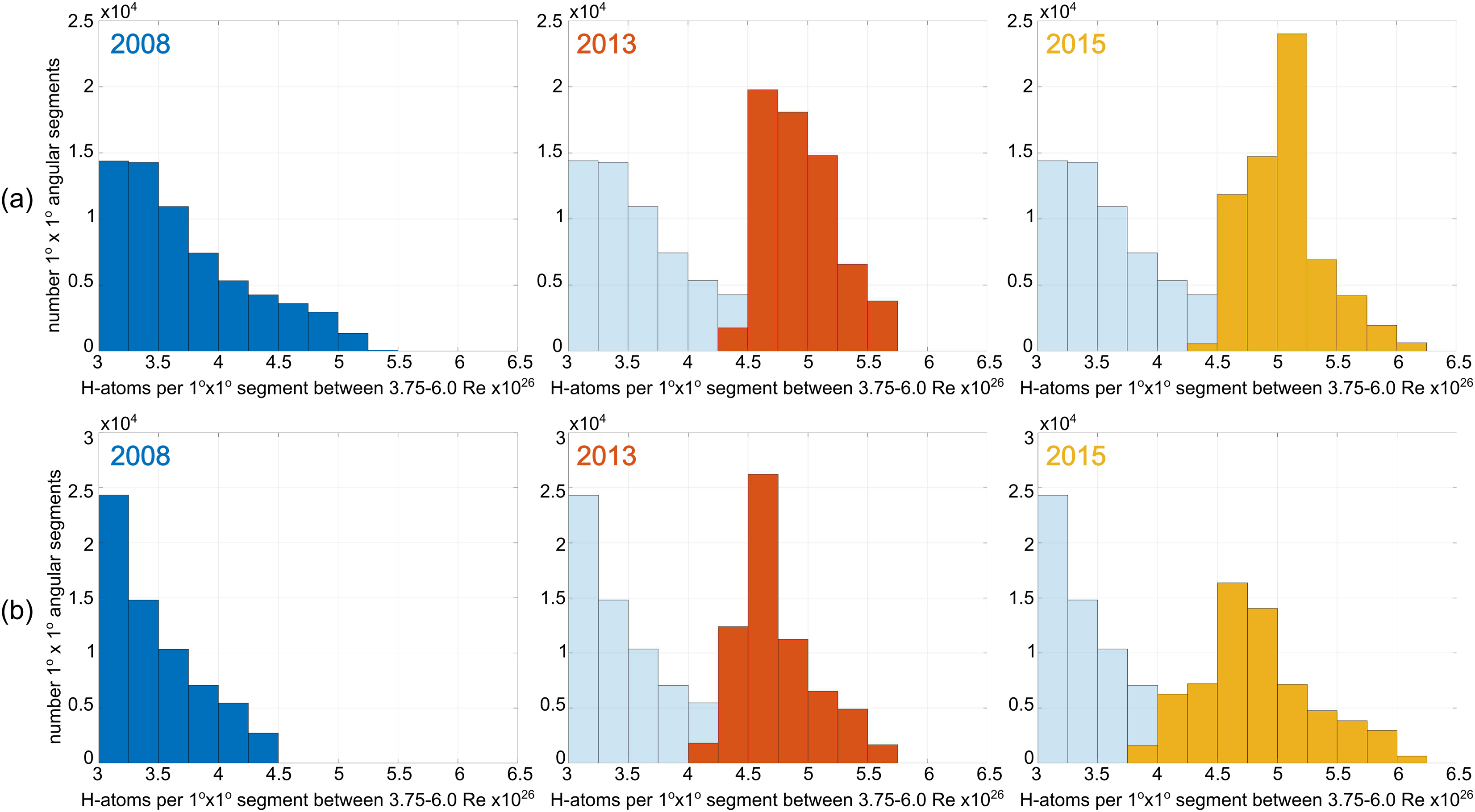
Figure 10. Histograms of the number of H-atoms (in 1 ° × 1 ° angular segments) between 3.75 and 6 Re for the inversions at solar minimum (2008) and maximum (2013 and 2015)—top row (A): based on the SHR model; bottom row (B): based on the “high degree-of-freedom” method.
In order to quantify the estimation error from both techniques (parametric fitting and “high degree-of-freedom” reconstruction), we calculate the relative inversion error or ratio of the observed to modeled LOS column brightness. Figure 11 shows histograms and the derived relative inversion errors (as the width of a Gauss fit) for each of the three datasets used in this study. A larger relative error in the 2015 dataset than that from the 2008 dataset is mainly due to the significant enhancement of instrumental noise as a result of the LAD sensitivity depletion. Since the count rates decrease similar to the decrease in sensitivity (in 2015 LAD1 by a factor of ∼7 and LAD2 by a factor of ∼3), the statistical error of the measurements increases accordingly. A second reason for the enhanced error in 2015 might be the large time span of the 2015 data selection, which covers 45 days (2008 = 1 day and 2013 = 20 days). Within these 45 days, the LADs can observe minor seasonal variations in the exosphere or variations due to the 27-day solar rotation cycle, which also increases the inversion error.
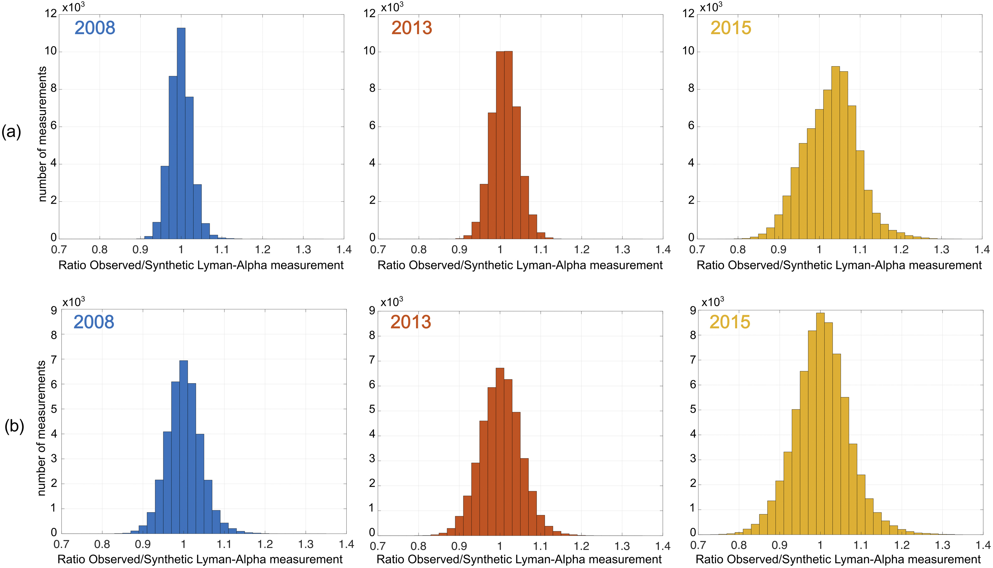
Figure 11. Histograms of the relative inversion error (ratio of the observed and modeled LOS column brightness) for the 3 years used—top row (A): based on the SHR model; bottom row (B): based on the “high degree-of-freedom” method. The relative errors are derived from Gauss curve fits of these histograms (top row: (A) 2008: 2.56%; 2013: 3.2%; and 2015: 6.4%; bottom row (B): 2008: 3.9%; 2013: 4.8%; and 2015: 6.0%). Larger relative errors in 2015 than in 2008 are mainly caused by the significant decrease in LAD sensitivity, which causes a higher statistical error in the observations due to accordingly reduced count rates. Furthermore, minor seasonal or solar rotation cycle-based exospheric H-density variations might contribute to the enhanced error in 2015, which has, with 45 days, the largest time span of all selections used (2008: 1 day; 2013: 20 days).
The uncertainty in the relative H-density enhancement at solar maximum (2013 or 2015) compared to solar minimum (2008) is calculated based on the following equation:
with the relative inversion errors of 2008
For the two inversion methods, the uncertainties in the H-density enhancements based on Equation 13 were found to be SHR 6.5% (2013) and 8.5% (2015) and HDOF 7.9% (2013) and 8.7% (2015). The average uncertainty for both methods and both solar max years is approximately 8%.
The SHR results for 12 June 2008 (solar minimum) can be compared to SHR results of the same day from an earlier analysis by Zoennchen et al. (2015), which was done with a lower angular resolution (L-order = 2) and a simple radial power law function. The solar minimum H-density distribution from this earlier work already shows both features, “nose” and “tail.” Nevertheless, the new results with the higher angular resolution, the better radial adaptation, and finally, the newly introduced regularization show deviations from the earlier results. The most obvious are a stronger “nose” feature and a significantly weaker “tail” in the presented results than those obtained by Zoennchen et al. (2015). Furthermore, the variation in the angular H density around the average value on a radial shell is generally lower in the new results.
The solar maximum results obtained by Zoennchen et al. (2015) are only partially comparable to those presented in this work. First, they are based on data from October to December 2012, meaning that they are from a different season and year (shortly before the solar maximum). Second, the data selection was not restricted to days with quiet geomagnetic conditions. However, the H-density enhancement of approximately +20% in 2012 found by Zoennchen et al. (2015) confirms the trend of higher H densities near the solar maximum.
4 Conclusion
The study of three independent datasets for solar minimum and maximum conditions enabled us to identify clear differences in the H density as a response to solar cycle 24. We summarize our scientific and technical findings as follows:
1. H-density distributions are, on average, ∼35 (±8)% higher during solar maximum than those under solar minimum conditions.
2. The presence of a nose/tail structure in all reconstructed models (see Figures 7, 8) is in good agreement with the radiation pressure theory, which establishes how the continuous scattering of Lyman-
3. Comparison between integrated H-atoms between solar minimum and solar maximum reconstructions reveals that the enhancement of the H population occurs from mid-to-high latitudes, with a preference for the dusk side (see Figure 9). Furthermore, only a ∼20% increase is seen near the SSP region, which has the highest H density and integrated H-atoms.
4. Analysis of the histograms of integrated H-atoms (see Figure 10) shows that the exosphere during solar maximum 2013 is more spherically symmetric than other reconstructions.
5. The use of two different and independent tomographic reconstruction techniques provides a high degree of confidence in the estimated H-density values.
6. Estimated errors in the tomographic reconstruction based on the comparison of observed and modeled column-integrated Lyman-alpha emission are ∼3–6% (see Figure 11). The average uncertainty in the LAD sensitivity decrease between 2008 and the solar maximum years 2013 and 2015 was found to be ∼5%
Our study provides important insights into the 3D structure of the exosphere. In this work, we included more sophisticated optical calibration and correction processes than in our previous studies (Zoennchen et al., 2015; Cucho-Padin and Waldrop, 2018). Furthermore, we compared two independent approaches for 3D reconstructions, and the results demonstrate excellent agreement, thereby providing confidence in the reported density values.
Structural differences between SHR and HDOF—caused by the different modeling techniques—can be summarized with a brighter nose and tail (particularly at the lower border) from the SHR inversion compared to the HDOF. However, regarding the principal validity of the main statements of this work (higher solar maximum H densities and similar angular features like nose, tail, or polar depletion), they are of minor significance. The continuously ongoing process of improving the model techniques will help minimize those structural differences.
Our results of higher H density during solar maximum than during solar minimum conditions contradict the findings from the physics-based model of the exosphere developed by Hodges (1994). Using an MC approach, this model includes an extensive number of reactions and interactions (e.g., between atomic H and several molecules and ions within the thermospheric and inner magnetospheric regions). Although the MC model exhibits spatial structures similar to our results, it has an evident opposite solar cycle dependence of the neutral H density at high altitudes (>2 Re) under similar solar conditions used in our study. On the other hand, the trend displayed by the density derived from the spherically symmetric Chamberlain model (Chamberlain, 1963) for both solar minimum and maximum is in better agreement with our results. Specifically, this model shows that at distances near the exobase (∼500 km), the H density is higher for solar minimum conditions than for solar maximum; however, this trend is reversed beyond ∼1.1 Re owing solely to the scale height effect for atomic H.
Nevertheless, we acknowledge that for a better interpretation of estimated H densities, data analysis may be assisted by physics-based modeling. Three drivers are crucial to define the exosphere structure: (a) the temperature and hydrogen density at the exobase region, which depend on the atmospheric (molecular and atomic) composition, winds in the thermosphere/mesosphere regions, and the solar radiation (Chamberlain, 1963); (b) the charge-exchange interaction with dense plasma regions such as the plasmasphere and magnetosheath (Kuwabara et al., 2017; Qin and Waldrop, 2016); and (c) solar radiation pressure, especially at high altitudes (Beth et al., 2016). A model that can account for these three mechanisms could be used to quantitatively identify the role of each of them in the exosphere formation. Furthermore, the identification of the energy partition of exospheric H-atoms is of great importance. Driver (a) defines the thermal population of atomic H that usually follows a Maxwellian distribution of 3D velocities with an average energy of ∼0.01 eV, while driver (b) produces the non-thermal H atoms with energies greater than 1 eV as plasma is usually hotter than neutrals. Investigation of the energization process will improve our understanding of the permanent upper-atmospheric escape to space.
Finally, this research work is timely and directly supports the upcoming NASA mission Carruthers Geocorona Observatory to be launched in 2025. This mission will image the terrestrial exosphere in Lyman-α with a wide field-of-view imager from the Sun–Earth L1 Lagrangian point (∼250 Re from Earth) and will be used to estimate the 3D global distributions of H densities, especially during solar maximum conditions. The description of our techniques in this paper may serve as guidance for software development, and the estimated H densities can be used as a first approximation ground-truth model to validate the estimation process.
Data availability statement
Publicly available datasets were analyzed in this study. These data can be found at: https://cdaweb.gsfc.nasa.gov/, https://lasp.colorado.edu/lisird/data/composite_lyman_alpha, http://omniweb.sci.gsfc.nasa.gov.
Author contributions
JZ: Conceptualization, writing–original draft and writing–review and editing. GC-P: Conceptualization, writing–original draft and writing–review and editing. LW: writing–review and editing. HF: writing–review and editing.
Funding
The author(s) declare that financial support was received for the research, authorship, and/or publication of this article. This research was supported by the Deutsche Forschungsgemeinschaft (grant no. 469043535) and the NASA Goddard Space Flight Center through Cooperative Agreement 80NSSC21M0180 to Catholic University, Partnership for Heliophysics and Space Environment Research (PHaSER).
Acknowledgments
The authors thank the TWINS team (PI Dave McComas) for making this work possible. Jochen Zoennchen acknowledges the funding by the Deutsche Forschungsgemeinschaft (DFG, German Research Foundation, grant no. 469043535) and the support of the Argelander Institut für Astronomie at the University of Bonn. Gonzalo Cucho-Padin thanks Drs. Dolon Bhattacharyya and John Clarke for important discussions on radiative transfer theory. The authors also acknowledge the International Space Science Institute on the ISSI team titled “The Earth’s Exosphere and its Response to Space Weather.” The authors thank the topical editor and the referees for the discussions for their extensive help in improving the paper.
Conflict of interest
The authors declare that the research was conducted in the absence of any commercial or financial relationships that could be construed as a potential conflict of interest.
The Editor DB is currently organizing a Research Topic with the author GC-P.
Publisher’s note
All claims expressed in this article are solely those of the authors and do not necessarily represent those of their affiliated organizations, or those of the publisher, the editors, and the reviewers. Any product that may be evaluated in this article, or claim that may be made by its manufacturer, is not guaranteed or endorsed by the publisher.
References
Bailey, J., and Gruntman, M. (2011). Experimental study of exospheric hydrogen atom distributions by Lyman-alpha detectors on the TWINS mission. J. Geophys. Res. Space Phys. 116 (19), 1–9. doi:10.1029/2011JA016531
Baliukin, I., Bertaux, J.-L., Quemerais, E., Izmodenov, V., and Schmidt, W. (2019). SWAN/SOHO Lyman-α mapping: the hydrogen geocorona extends well beyond the Moon. J. Geophys. Res.-Space 124, 861–885. doi:10.1029/2018JA026136
Beth, A., Garnier, P., Toublanc, D., Dandouras, I., and Mazelle, C. (2016). Theory for planetary exospheres: I. Radiation pressure effect on dynamical trajectories. Icarus 266, 410–422. doi:10.1016/j.icarus.2015.10.018
Bishop, J. (1999). Transport of resonant atomic hydrogen emissions in the thermosphere and geocorona: model description and applications. J. Quantitative Spectrosc. Radiat. Transf. 61, 473–491. doi:10.1016/S0022-4073(98)00031-4
Bishop, J., and Chamberlain, J. W. (1989). Radiation pressure dynamics in planetary exospheres: a “natural” framework. Icarus 81, 145–163. doi:10.1016/0019-1035(89)90131-0
Brandt, J. C., and Chamberlain, J. W. (1959). Interplanetary gas. I. Hydrogen radiation in the night sky. Astrophysical J. 130, 670–682. doi:10.1086/146756
Butala, M. D., Hewett, R. J., Frazin, R. A., and Kamalabadi, F. (2010). Dynamic three-dimensional tomography of the solar corona. Sol. Phys. 262, 495–509. doi:10.1007/s11207-010-9536-1
Chamberlain, J. W. (1963). Planetary coronae and atmospheric evaporation. Planet. Space Sci. 11, 901–960. doi:10.1016/0032-0633(63)90122-3
Connor, H. K., and Carter, J. A. (2019). Exospheric neutral hydrogen density at the nominal 10 RE subsolar point deduced from xmm-Newton X-ray observations. J. Geophys. Res.-Space 124, 1612–1624. doi:10.1029/2018JA026187
COSPAR. Working Group IV (1965). Cira 1965: COSPAR international reference atmosphere 1965, COSPAR series. North-Holland Publishing Company. doi:10.1038/2101305a0
Cucho-Padin, G., Connor, H., Jung, J., Walsh, B., and Sibeck, D. G. (2024). Finding the magnetopause location using soft x-ray observations and a statistical inverse method. Earth Planet. Phys. 8, 184–203. doi:10.26464/epp2023070
Cucho-Padin, G., Kameda, S., and Sibeck, D. G. (2022). The earth’s outer exospheric density distributions derived from procyon/laica uv observations. J. Geophys. Res. Space Phys. 127, e2021JA030211. doi:10.1029/2021JA030211
Cucho-Padin, G., and Waldrop, L. (2018). Tomographic estimation of exospheric hydrogen density distributions. J. Geophys. Res. Space Phys. 123 (Issue 6), 5119–5139. doi:10.1029/2018ja025323
Cucho-Padin, G., and Waldrop, L. (2019). Time-dependent response of the terrestrial exosphere to a geomagnetic storm. Geophys. Res. Lett. 46, 11661–11670. doi:10.1029/2019GL084327
Emerich, C., Lemaire, P., Vial, J.-C., Curdt, W., Schühle, U., and Wilhelm, K. (2005). A new relation between the central spectral solar HI Lyman-α irradiance and the line irradiance measured by SUMER/SOHO during the cycle 23. Icarus 178, 429–433. doi:10.1016/j.icarus.2005.05.002
Emmert, J. T., Drob, D. P., Picone, J. M., Siskind, D. E., Jones, M., Mlynczak, M. G., et al. (2021). NRLMSIS 2.0: a whole-atmosphere empirical model of temperature and neutral species densities. Earth Space Sci. 8, e2020EA001321. doi:10.1029/2020EA001321
Fahr, H. J. (1971). The interplanetary hydrogen cone and its solar cycle variations. Astron. Astrophys. 14, 263–274.
Fahr, H. J., Nass, U., Dutta-Roy, R., and Zoennchen, J. H. (2018). Neutralized solar wind ahead of the Earth’s magnetopause as contribution to non-thermal exospheric hydrogen. Ann. Geophys. 36, 445–457. doi:10.5194/angeo-36-445-2018
Feller, W. (1968). An introduction to probability theory and its applications. New York, USA: Wiley.
Fuselier, S. A., Dayeh, M. A., Galli, A., Funsten, H. O., Schwadron, N. A., Petrinec, S. M., et al. (2020). Neutral atom imaging of the solar wind-magnetosphere-exosphere interaction near the subsolar magnetopause. Geophys. Res. Lett. 47, e2020GL089362. doi:10.1029/2020GL089362
Hodges, R. R. (1994). Monte Carlo simulation of the terrestrial hydrogen exosphere. J. Geophys. Res. Space Phys. 99, 23229–23247. doi:10.1029/94JA02183
Joshi, P. P., Phal, Y. D., and Waldrop, L. S. (2019). Quantification of the vertical transport and escape of atomic hydrogen in the terrestrial upper atmosphere. J. Geophys. Res. Space Phys. 124, 10468–10481. doi:10.1029/2019JA027057
Krall, J., Glocer, A., Fok, M. C., Nossal, S. M., and Huba, J. D. (2018). The unknown hydrogen exosphere: Space weather implications. Space Weather. 16, 205–215. doi:10.1002/2017SW001780
Kuwabara, M., Yoshioka, K., Murakami, G., Tsuchiya, F., Kimura, T., Yamazaki, A., et al. (2017). The geocoronal responses to the geomagnetic disturbances. J. Geophys. Res. Space Phys. 122, 1269–1276. doi:10.1002/2016JA023247
McComas, D. J., Allegrini, F., Baldonado, J., Blake, B., Brandt, P. C., Burch, J., et al. (2009). The two wide-angle imaging neutral-atom Spectrometers (TWINS) NASA mission-of-opportunity. Space Sci. Rev. 142 (1–4), 157–231. doi:10.1007/s11214-008-9467-4
Nass, H. U., Zoennchen, J. H., Lay, G., and Fahr, H. J. (2006). The TWINS-LAD mission: observations of terrestrial Lyman-α fluxes. ASTRA Astrophysics Space Sci. Trans. 2, 27–31. doi:10.5194/astra-2-27-2006
Norberg, J., Käki, S., Roininen, L., Mielich, J., and Virtanen, I. I. (2023). Model-free approach for regional ionospheric multi-instrument imaging. J. Geophys. Res. Space Phys. 128, e2022JA030794. doi:10.1029/2022JA030794
Norberg, J., Vierinen, J., Roininen, L., Orispää, M., Kauristie, K., Rideout, W. C., et al. (2018). Gaussian markov random field priors in ionospheric 3-d multi-instrument tomography. IEEE Trans. Geoscience Remote Sens. 56, 7009–7021. doi:10.1109/tgrs.2018.2847026
Østgaard, N., Mende, S. B., Frey, H. U., Gladstone, G. R., and Lauche, H. (2003). Neutral hydrogen density profiles derived from geocoronal imaging. J. Geophys. Res. Space Phys. 108 (A7), 1–12. SMP 18. doi:10.1029/2002JA009749
Qin, J., and Waldrop, L. (2016). Non-thermal hydrogen atoms in the terrestrial upper thermosphere. Nat. Commun. 7, 13655. doi:10.1038/ncomms13655
Rairden, R. L., Frank, L. A., and Craven, J. D. (1986). Geocoronal imaging with dynamics explorer. J. Geophys. Res. Space Phys. 91, 13613–13630. doi:10.1029/ja091ia12p13613
Snow, M., Reberac, A., Quémerais, E., Clarke, J., McClintock, W. E., and Woods, T. N. (2013). A new catalog of ultraviolet stellar spectra for calibration. ISSI Sci. Rep. Ser. 13, 191–226. doi:10.1007/978-1-4614-6384-9_7
Thomas, G. E. (1978). The interstellar wind and its influence on the interplanetary environment. Annu. Rev. earth Planet. Sci. 6, 173–204. doi:10.1146/annurev.ea.06.050178.001133
Vidal-Madjar, A. (1975). Evolution of the solar Lyman alpha flux during four consecutive years. Sol. Phys. 40, 69–86. doi:10.1007/BF00183153
Waldrop, L., and Paxton, L. J. (2013). Lyman-α airglow emission: implications for atomic hydrogen geocorona variability with solar cycle. J. Geophys. Res. Space Phys. 118, 5874–5890. doi:10.1002/jgra.50496
Zoennchen, J. H., Connor, H. K., Jaewoong, J., Nass, U., and Fahr, H. J. (2022). Terrestrial exospheric dayside H-density profile at 3–15 Re from UVIS/HDAC and TWINS Lyman-α data combined. Ann. Geophys. 40, 271–279. doi:10.5194/angeo-40-271-2022
Zoennchen, J. H., Nass, U., and Fahr, H. J. (2015). Terrestrial exospheric hydrogen density distributions under solar minimum and solar maximum conditions observed by the TWINS stereo mission. Ann. Geophys. 33, 413–426. doi:10.5194/angeo-33-413-2015
Keywords: exosphere, solar cycle, atmospheric escape, parametric estimation, tomographic estimation
Citation: Zoennchen JH, Cucho-Padin G, Waldrop L and Fahr HJ (2024) Comparison of terrestrial exospheric hydrogen 3D distributions at solar minimum and maximum using TWINS Lyman-α observations. Front. Astron. Space Sci. 11:1409744. doi: 10.3389/fspas.2024.1409744
Received: 30 March 2024; Accepted: 24 September 2024;
Published: 16 October 2024.
Edited by:
Dolon Bhattacharyya, University of Colorado Boulder, United StatesReviewed by:
Nickolay Ivchenko, Royal Institute of Technology, SwedenVladimir A. Sreckovic, University of Belgrade, Serbia
Copyright © 2024 Zoennchen, Cucho-Padin, Waldrop and Fahr. This is an open-access article distributed under the terms of the Creative Commons Attribution License (CC BY). The use, distribution or reproduction in other forums is permitted, provided the original author(s) and the copyright owner(s) are credited and that the original publication in this journal is cited, in accordance with accepted academic practice. No use, distribution or reproduction is permitted which does not comply with these terms.
*Correspondence: Jochen H. Zoennchen, em9lbm5AYXN0cm8udW5pLWJvbm4uZGU=
 Jochen H. Zoennchen
 Gonzalo Cucho-Padin
 Lara Waldrop4
 Hans J. Fahr