 Rachel Frissell
 Hyomin Kim2
 Nathaniel Frissell
- 1University of Scranton, Scranton, PA, United States
- 2Department of Physics and Engineering, New Jersey Institute of Technology, Newark, NJ, United States
It has been shown that a proxy determination of the magnetospheric open–closed magnetic field line boundary (OCB) location can be made by examining the ultra-low-frequency (ULF) wave power in magnetometer data, with particular interest in the Pc5 ULF waves with periods of 3–10 min. In this study, we present a climatology of such Pc5 ULF waves using ground-based magnetometer data from the South Pole Station (SPA), McMurdo (MCM) station, and the Automatic Geophysical Observatories (AGOs) located across the Antarctic continent, to infer OCB behavior and variability during geomagnetically quiet times (i.e., Ap < 30 nT). For each season [i.e., austral fall (20 February 2017–20 April 2017), austral winter (20 May 2017–20 July 2017), austral spring (20 August 2017–20 October 2017), and austral summer (20 November 2017–20 January 2018)], north–south (i.e., H-component) magnetic field line residual power–spectral density (PSD) measurements taken during geomagnetically quiet periods within a 60-day window centered at the austral solstice/equinox are averaged in 10-min temporal bins to form the climatology at each station. These residual PSDs thus enable the analysis of Pc5 activity (and lower period “long-band” oscillations) and, thus, OCB location/variability as a function of season and magnetic latitude. The dawn and dusk transitions across the OCB are analyzed, with a discussion of dawn and dusk variability during nominally quiet geomagnetic periods. In addition, latitudinal dependencies of the OCB and peak Pc5 periods at each station are discussed, along with the empirical Tsyganenko model comparisons to our site measurements.
1 Introduction
The high-latitude region where the transition of an area of open magnetic field lines to closed magnetic field lines takes place is called the open–closed boundary (OCB). In this study, we define a closed magnetic field line as the one that leaves the Southern Hemisphere and terminates in the Northern Hemisphere, as shown in Figure 1A [with the field line traced from the Tsyganenko (1989) model, hereafter referred to as T89]. Conversely, we define an open field line as one that does not terminate in the opposite hemisphere, as shown in Figure 1B. When Earth’s magnetic field lines interact with the interplanetary magnetic field (IMF) dragged outward by the solar wind, closed field lines can open, and vice versa, in a process generally described as magnetic reconnection or field line merging. In addition, seemingly open field lines may actually be closed far down the magnetotail or in the magnetolobes (e.g., Cowley, 1981).
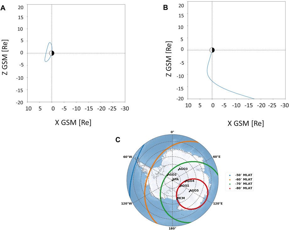
Figure 1. Magnetic field line traces from the T89 model for 12 UT on 3/20/17. (A) Closed magnetic field line trace as predicted by the T89 model at AGO3. Day and night are represented by white and black shading, respectively. (B) Open magnetic field line trace as predicted by the T89 model at AGO5. (C) Map representing the locations of AGO1, AGO2, AGO3, AGO5, McMurdo (MCM), and South Pole (SPA). The magnetic latitude lines, which are represented by various colored lines, are overlaid for reference. The red circle represents the highest magnetic latitude of −80°, followed by green, orange, and blue, which is the lowest magnetic latitude at −50°. The gray dotted lines represent the geographic latitude lines.
Substantial research has been conducted on magnetospheric OCB physics and dynamics and the OCB itself, and its changes in time/variability can be a proxy for a number of compelling space weather-related issues. For example, under unbalanced magnetic merging, the mean dayside merging lacks a fully compensating nightside merging (Siscoe and Huang, 1985). The amount of open magnetic flux then increases, and the polar cap, defined as the sum area of all open magnetic field lines, would inflate. Conversely, the polar cap would deflate when open field lines closed during tail merging. Thus, many studies of the OCB variability are tied to the underlying dynamics of field line reconnection/merging [e.g., Milan et al. (2003) and Lockwood et al. (2005) studied the relationship between the dayside polar cap boundary and substorm phase; Kamide et al. (1999) considered the effects of solar wind and IMF parameters on the polar cap area], and much work has been done using different techniques to infer or measure the OCB [e.g., Sotirelis et al. (1998) inferred the OCB using auroral crossings from four Defense Meteorological Satellite Program (DMSP) satellites; Wild et al. (2004) combined both space- and ground-based observations to infer the dawn-sector auroral zone and, thus, the OCB; Baker et al. (1995) used SuperDARN radars to relate the signatures of the cusp and low-latitude boundary layer with DMSP satellite OCB observations; Longden et al. (2010) developed an automated method from far ultraviolet images of the aurora to determine the location of the poleward auroral luminosity boundary and, thus, the OCB; Newell and Meng (1988) used particle measurements obtained by LEO satellites; and Gallardo-Lacourt et al. (2022) used redline optical data].
Regarding ground-based magnetometer data, studies of the propagation and resonance characteristics of observed ULF waves are a useful diagnostic tool for understanding the dynamic magnetosphere and its plasma from both a spatial and temporal perspective (Fraser, 2009). Regarding OCB detection methodologies, Lanzerotti et al. (1999) found that narrow spectral bands in north–south (i.e., H-component)-oriented magnetic field line PSDs with periods in the Pc5 ULF band (nominally between 2.5- and 10-min periods) can provide an insight into the location of the OCB. Lessard et al. (2009) used such magnetometer PSDs to determine the OCB, following a March 23 substorm. This dataset was compared to a numerical estimate of the OCB by the Block-Adaptive-Tree Solar wind Roe-type Upwind Scheme (BATSRUS) with good agreement. Urban et al. (2011) also found good agreement with the BATSRUS model and noted that the synoptic variability of the OCB morphology could be well-traced using an array of Antarctic magnetometers. Pilipenko et al. (2015) and Pilipenko et al. (2017) combined radar and optical data with latitudinal chains of magnetometers for the OCB identification and found that the latitudinal peak of broadband dayside Pc5 pulsation spectra is not under the proper cusp but several degrees southward from the equator-ward cusp boundary. Additionally, Kozyreva et al. (2019) suggested that the near-noon proxy of the OCB is related to the high-latitude transient Pc5 pulsations rather than long-lasting broadband pulsations. We note that the outcomes of these later studies indicate that the location of the OCB from ground-based magnetometer systems can have a latitudinal uncertainty of <5° and is not relevant to the outcomes of this study.
In this paper, we present a climatology of Pc5 ULF waves measured using an array of ground-based magnetometers from the South Pole Station (SPA), McMurdo (MCM) station, and the Automatic Geophysical Observatories (AGOs), located across the Antarctic continent, to infer OCB behavior and variability during geomagnetically quiet times. This is done for all four austral seasons in 2017, where sufficient data from all the stations existed for comparison. Section 2 discusses the instrumentation, datasets, data processing, and overall analysis methodology. Section 3 presents the residual PSD climatology for each station for the four solstice/equinoctial periods. Section 4 presents a comparison to the T89 model, a discussion on the dawn and dusk transitions, and a discussion of ULF wave characteristics with latitudinal variations. Section 5 provides the conclusion with key points and takeaways.
2 Instrumentation, datasets, data processing, and methodology
The Polar Engineering Development Center at the New Jersey Institute of Technology operates and manages geospace instruments at the SPA station, MCM station, Palmer Station, and at the AGOs, named AGO1, AGO2, etc. These sites are unique as they are located over an expansive region, are conjugate with the Northern Hemisphere, and contain sites deep into the polar cap. Their geographic and geomagnetic latitudes and longitudes are listed in Table 1, and Figure 1C shows their relative locations. AGO1, AGO4, and MCM station all are approximately along the red circle representing a magnetic latitude of −80°. SPA and AGO3 are both between the red and green circles (representing magnetic latitude of −70°). AGO2 is the lowest magnetic latitude, sitting on the green circle that represents a magnetic latitude of −70°. The Universal time (UT) to magnetic local time (MLT) conversion is provided for each of the stations, and all results herein are presented in MLT with the conversion done through aacgmV2 (Burrell et al., 2020; Shepherd, 2014). We note that although instrumentation operating at the manned stations can use that infrastructure for reliable data transmission, the remote AGO systems rely on remote solar and wind power and iridium contacts. Thus, the operation of these remote facilities is associated with greater data gaps. Although all data are saved on site in the AGO enclosures, retrieving such data requires flight resources that have substantially reduced in the past 15 years. Thus, AGO4, for example, has been extremely impacted and included here only for completeness.
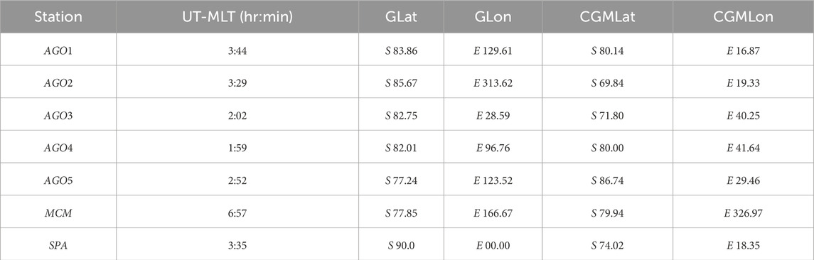
Table 1. Conversion for UT to MLT time, and geographic and geomagnetic coordinates.
Magnetic fluxgate data from all three field line components from SPA and MCM stations are recorded every second. In comparison, data from the AGO sites report only magnetic fluxgate north–south (i.e., H-component) magnetic field data with a 20-s (±5 s) cadence. All data are binned into 20-s nominal realizations, and short (
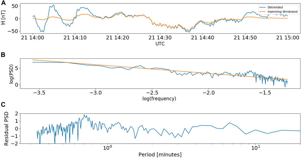
Figure 2. Overview of the calculation of the residual PSD. (A) 60-min long sample of H-component magnetometer data from AGO3 (blue trace) and windowed with a 60-min long Hamming window (orange trace). (B) The PSD from these windowed data, approximated by the periodogram defined as the magnitude squared of the Fourier transform of the windowed data, is represented by the blue trace. A least-squares best fit straight line of the PSD in the log of PSD amplitude-log PSD frequency (i.e., log–log domain) is indicated by the orange trace. (C) Subtracting the best fit straight line from the PSD generates the residual PSD, presented in period. This sequence is reported for each 60-min window, slid forwarding in time in 10-min increments, over a 24-h day, with beginning and ending time periods of the day taken from the previous and following day’s data.
For each station, we estimated the first and (square root) second moments (i.e., the mean and standard deviation, respectively) of the 24-h residual spectrograms that were 1) obtained during a quiet-time geomagnetic conditions and 2) measured in a 60-day period window within each of the four “cardinal seasons,” defined here as the austral fall equinox (20 February 2017–20 April 2017), austral winter solstice (20 May 2017–20 July 2017), austral spring equinox (20 August 2017–20 October 2017), and austral summer solstice (20 November 2017–20 January 2018). Herein, we define geomagnetically quite time periods (i.e., quiet time) as any day on which the corresponding Ap value, that is, the daily average of ap values from the NASA OMNI dataset, was less than 30 nT. Thus, site-specific and season residual spectrograms of average residual Pc5 energy and the standard deviation of the residual Pc5 energy, as a function of the 24-h day, were obtained for quiet-time conditions, and examples of the average spectrograms are given in Figure 3.
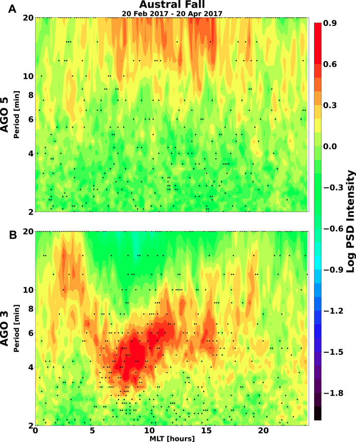
Figure 3. Average quiet-time residual PSD spectrograms for (A) AGO5 and (B) AGO3 for austral fall (20 February 2017–20 April 2017). AGO5 under continuously open magnetic field lines, typical of a station deep in the polar cap. AGO3 sits at a lower magnetic latitude than AGO5 and transitions between open and closed field lines through the day. A dot indicates an MLT/period where the climatological residual PSD energy varied by more than one standard deviation over the 60-data window.
Herein, the residual PSD spectrograms are discussed regarding two frequency bands: the Pc5 and long-period (LP) oscillation band. Pc5 waves have periods between 150 and 600 s or 2.5 and 10 min Jacobs et al. (1964), while LP waves typically have periods of 10 min or greater (Lanzerotti et al., 1999; Urban et al., 2011). It is expected that during nighttime, LP waves will have high power and typically indicate long, extended closed magnetotail field lines. Urban et al. (2011) stated that LP waves are not expected in daytime, and higher power in Pc5 waves is indicative of closed field lines. As nighttime transitions to daytime, a transition from field lines exhibiting LP oscillations to field lines only exhibiting Pc5 waves would be seen. Additionally, LP waves have been also denoted as irregular pulsations at cusp latitudes (IPCLs) Troitskaya and Bolshakova (1977) and have been associated with broadband Pc5 pulsations (McHarg et al., 1995; Posch et al., 1999; Engebretson et al., 2006). Note that longer-period quasi-periodic fluctuations at high latitude can also be observed in relation to direct driving from the solar wind (De Lauretis et al., 2016; Di Matteo et al., 2022) or magnetopause surface waves (Kozyreva et al., 2019).
Figure 3 presents a typical residual PSD spectrogram climatology for AGO5, a deep polar-cap site almost always on open field lines, and AGO3, an auroral site that regularly transitions across the OCB, for austral fall 2017 for quite geomagnetic conditions. At AGO3, one sees the dawn–day–dusk transitions in the wave activity signature. Urban et al. (2011) previously described this feature as a “swooping U.” The first half of the “swooping U” is seen in the dawn sector from 3 to 9 MLT, where wave energy progresses from LP oscillations into the Pc5 range. This is a transition from open field lines to closed field lines. As one progresses throughout the day (i.e., 9 to 15 MLT), one would expect to see an extended interval of isolated Pc5 due to the continuous presence of closed field lines. Of particular note at AGO3 is that the lowest periods are not seen at 12 MLT but rather, at 7–8 MLT. This feature is seen at other sites and discussed more later. At MLT dusk (15–21 MLT), the Pc5 periods slowly disappear from the residual spectrogram, indicative of the site progressing from closed to open field lines. At AGO5, however, one observes the absence of Pc5 waves, consistent of a deep polar cap site (Urban et al., 2016).
The black dots in Figure 3 indicate time/periods that, over the 60-day austral fall 2017 period of time, the residual power spectrum values had a standard deviation greater than 1-sigma. In other words, the residual PSD energy at times/periods that fluctuated more than 68 (“%”) about the average for that time/period over the 60-day period is “flagged” by a black dot, under the assumption of Gaussian statistics. Thus, the black dots represent times/periods of greater variability. Figure 3 shows that there is substantial variability across the Pc5 range between 6 and 9 MLT, the dawn sector. There is less variability at other AGO3 MLTs and similar at AGO5 for all MLTs, as inferred by a lack of clustering of dots. We see these same trends at other sites at equivalent magnetic latitudes herein.
3 Observations
Figure 4 shows the quiet-time residual PSD climatology of oscillations in the Pc5 and LP bands measured from the six Antarctic stations for the four “cardinal seasons.” On immediate inspection, one can observe the impact the magnetic latitude has on the presence of the “swooping U” LP to Pc5 to the LP signature. AGO2 and AGO3 both sit at a lower magnetic latitude than SPA, and all three stations clearly display the “U.” Meanwhile, stations at higher latitudes do not display such a structure, as would be expected from a site not passing under the OCB.
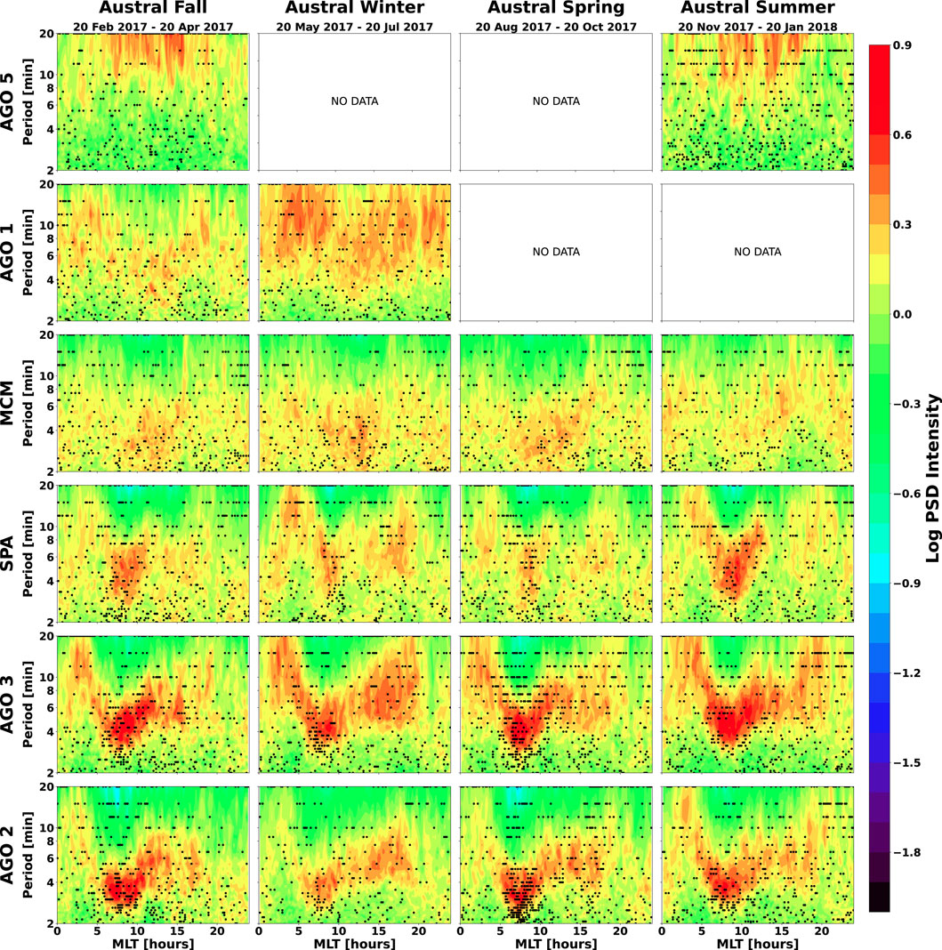
Figure 4. Climatological quiet-time residual PSD spectrograms for the four “cardinal seasons” for [top to bottom] AGO5, AGO1, MCM, SPA, AGO3, and AGO2. A dot indicates an MLT/period where the climatological residual PSD energy varied by more than one standard deviation over the 60-data window.
At the highest magnetic latitudes, sited deep in the polar cap, AGO5 is continuously in a region of open field lines, as demonstrated by the absence of Pc5 waves. Of interest is the increase in LP power at AGO5 between 6 and 18 MLT, centered around 12 MLT (i.e., magnetic noon), where the field lines are nominally greatly extended behind Earth.
At lower latitudes, we commonly say that MCM and AGO1 both sit at approximately −80°. However, the spectrograms for these stations given in Figure 4 show a slight shift of higher residual power toward slightly longer periods at AGO1 compared to MCM, demonstrating the very slight but measureable difference in magnetic latitude, with AGO1 at 80.14° and MCM at 79.94°. In fact, one can almost start to see the “swooping U” in the MCM residual PSDs, again a clear indication that the common adage that “MCM is in the polar cap” is inappropriate.
For austral winter 2017, AGO1 shows signatures of both LP waves and Pc5 waves from 0 to 8 MLT. At the same time, MCM only shows a signature of Pc5 waves during the same time. The signature between 8 and 14 MLT appears very similar for both AGO1 and MCM. Between 14 and 24 MLT, AGO1 again shows both LP and Pc5 waves present, while MCM generally only shows Pc5 signatures. However, in austral spring and summer, MCM shows both Pc5 and LP waves, much like AGO1 in austral fall/winter. It is unfortunate that we did not have austral spring and summer data from AGO1 for comparison.
At even lower magnetic latitudes, SPA, and then AGO2/AGO3, one sees many of the same features shown in Figure 3 in reference to AGO3, specifically, the first half of the “swooping U” in the dawn sector from 3 to 9 MLT, where wave energy progresses from LP oscillations into the Pc5 range. As one progresses throughout the day (i.e., 9 to 15 MLT), one sees an extended interval of isolated Pc5 due to the continuous presence of closed field lines. Again, the lowest periods are not seen at 12 MLT but rather, at 7–8 MLT at all three of these sites. One also sees that there is substantial variability across the Pc5 range between 6 and 9 MLT, i.e., the dawn sector. There is less variability at other MLTs.
In an effort to quantify the spectrogram variability in the 3–15 MLT time interval, in Figure 5, we plot the value of the period that had the maximum residual PSD energy, within a 1-h window, for MCM, SPA, AGO3, and AGO2. Although it is difficult to see trends in the period of peak energy for MCM and SPA, the asymmetry in the periods is observed at AGO2 and AGO3, with a minimum period of peak energy occurring at 9 MLT, which would be considered the dawn–noon flank. Figure 5 thus highlights the asymmetry in periodicity seen in the dawn-to-noon-to-dusk transitions seen on inspection in Figure 4. In addition, Figure 5 shows that the periods of peak energy at AGO2 are at lower values that those seen at AGO3, which would be reasonable given that AGO3 is at a slightly higher geomagnetic latitude than AGO2. The analysis of Figure 5 for AGO2 and AGO3 is repeated using spectrally and temporally smoothed data (
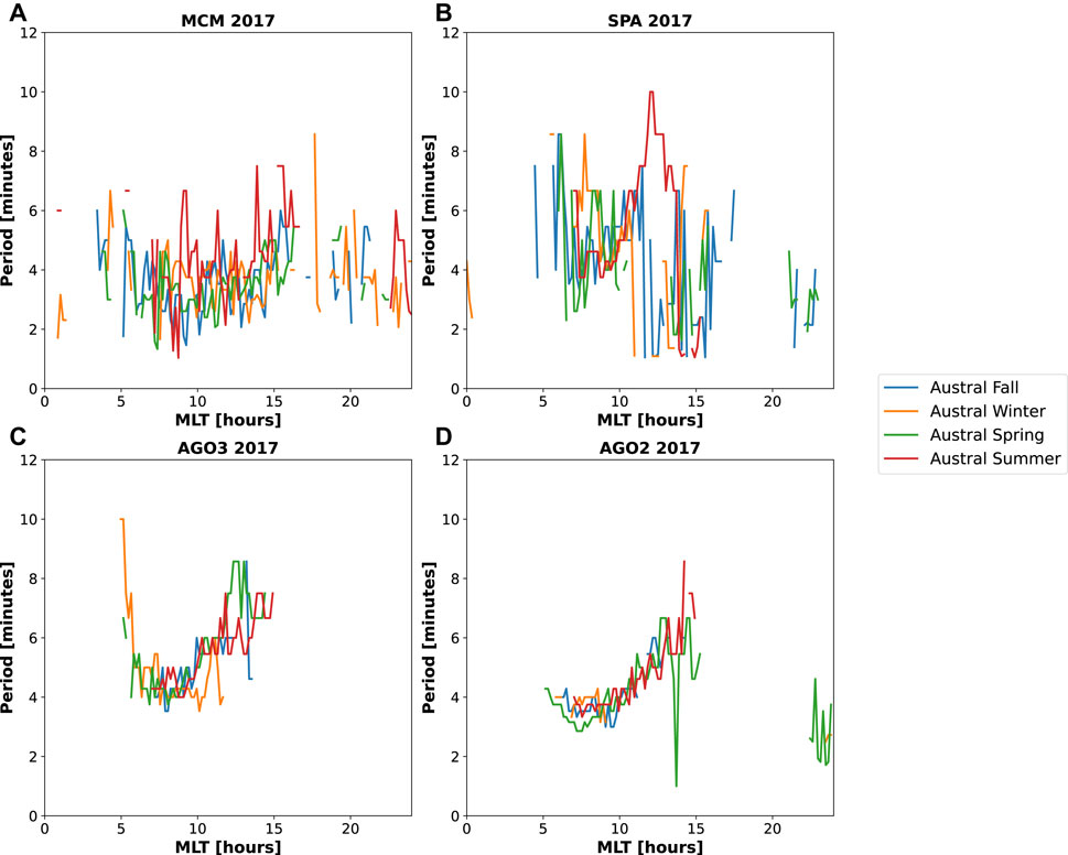
Figure 5. Temporal variation in the period with maximum residual PSD energy, organized by a station for the four “cardinal seasons.” AGO1 and AGO5 are not shown due to limited data and values outside of the selected range of periods between 1 and 20 min. (A) MCM, (B) SPA, (C) AGO3, and (D) AGO2.
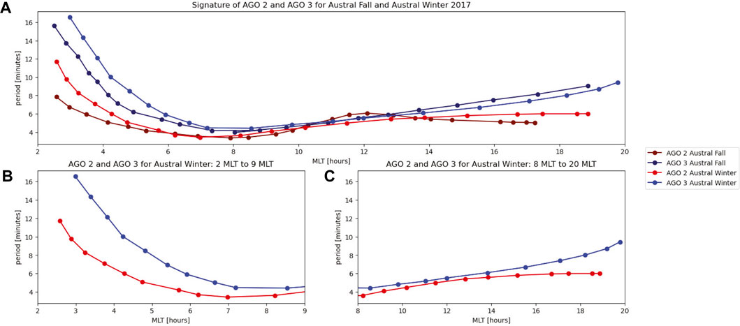
Figure 6. (A) The asymmetry between dawn and dusk of the period at the center of the broad enhancement of residual PSD from AGO2 and AGO3 is presented using spectrally/temporally smoothed versions of data in Figure 4. These data highlight the difference in the slope of the “swooping U” signature from (B) 2 MLT to 9 MLT, which is quite steep, and (C) 8 MLT to 20 MLT, which is much less so.
4 Discussion
4.1 OCB determination and the Tsyganenko model
To test the general climatological results presented in Figure 4, we compare our station location/measurements to the empirical T89 model in Figure 7, which was run at 3, 12, and 21 UT on March, June, September, and December 20 (i.e., austral fall, winter, spring, and summer) for low Kp (Kp
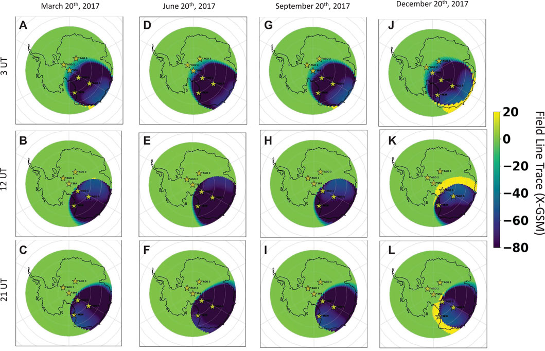
Figure 7. Comparison of station location/field measurements to the empirical T89 model at 3 (A,D,G,J), 12 (B,E,H,K), and 21UT (C,F,I,L) on March (A–C), June (D–F), September (G–I), and December 20 (J–L) (i.e., austral fall, winter, spring, summer) for low Kp (Kp = 2), for an array of surface latitude/longitude points mapped outward. The final field line x-GSM value, measured in Earth radii, is depicted by color. A closed field line will typically have a positive (dayside facing) or negative (nightside facing) x-GSM field line location of absolute magnitude
Regarding AGO2 and AGO3, both Figures 4, 7 suggest that these stations are regularly located on a closed magnetic field line because of the “swooping U” signature and clear Pc5 waves. Figure 7 further supports this for nearly all seasons and UTs/MLTs. AGO5 is clearly deep in the polar cap in Figure 7. Meanwhile, for SPA, the station finds itself often passing under the OCB. In other words, we expect closed field lines for 12 UT and 21 UT, with open field lines at 3 UT. AGO1 and MCM would be similarly transitioning as SPA does but less frequently and more dependent on variations in the solar wind.
4.2 Dawn and dusk transitions
The structure initially defined as the “swooping U” given in Figures 3, 4 is not symmetric, with the dawn transition being much steeper than the dusk transition. This asymmetry can be easily seen in Figure 6, with a steeper transition at dawn than dusk. The same dawn–dusk asymmetry is also seen in the T89 model output. Although dawn–dusk asymmetries are well-documented, the exact cause is beyond the scope of this effort.
4.3 Seasonal and latitudinal variation
Greater ULF energy is observed at lower-magnetic latitude sites during equinoctial conditions, as shown in Figure 4. We speculate that this is associated with the enhanced magnetosphere–ionosphere coupling efficiencies associated with the “dipole tilt,” which may be defined as the angle between the geomagnetic dipole axis and the geocentric solar magnetosphere z-axis, also known as the Russell–McPherron effect, which hypothesizes an increase in the average energy injected into the magnetosphere at equinoctial periods due to the right-angle tilt in relation to the solar wind (Russell and McPherron, 1973; Zhao and Zong, 2012). Although the exact physical mechanism of this magnetosphere–ionosphere coupling is open, it is reasonable to assume that enhanced ULF energy on closed field lines would be associated with enhanced solar wind coupling (Cnossen et al., 2012).
Figure 5 also shows latitudinal variation. The lowest period with the maximum amplitude decreases in value, as organized by the station, MCM, SPA, AGO3, and then AGO2, as magnetic latitude decreases. Additionally, Figure 6 shows the impact of the slight latitudinal variation between AGO2 and AGO3. Although both have asymmetry in the “swooping U,” the slope of the dawn transition for AGO3 is steeper than for AGO2. We also note that the dusk transition varies in period based on the magnetic latitude of a particular site. Such would be expected, given the nature of field-line resonances.
5 Conclusion
Herein, a geomagnetically quiet-time residual PSD climatology of Pc5 and LP waves, used to infer open and closed field lines, was presented. These data came from stations across the Antarctic continent, with many at unmanned locations operating autonomously. The data were used to study OCB behavior during such quiet periods in an effort to better understand the naturally occurring dynamics of the region without storm-time influences. Under such conditions, we generally find that 1) LP and Pc5 waves seem to be reliable tracers of the OCB, within uncertainties of a few degrees, and are compatible with estimates of the OCB locations obtained from empirical models; 2) lower-magnetic latitude stations clearly show the characteristic “swooping U” structure, and most of its variability is in the dawn sector; 3) the “U” structure is asymmetrical, being much steeper in the dawn sector than the dusk sector. Thus, the letter “U” is inappropriate, given the asymmetry, and a different letter, like
Data availability statement
The datasets presented in this study can be found in online repositories. The names of the repository/repositories and accession number(s) can be found in the article/Supplementary Material.
Author contributions
RF: writing–original draft. HK: writing–review and editing. AG: writing–original draft. NF: writing–review and editing.
Funding
The author(s) declare that financial support was received for the research, authorship, and/or publication of this article. This work was supported by the National Science Foundation Office of Polar Programs, grants PLR-1247975 and PLR-1443507, which partially support AGO field operations on the Antarctican plateau, and OPP-1744861, OPP-2032421, and OPP-1643700 which support polar cap dynamics studies.
Conflict of interest
The authors declare that the research was conducted in the absence of any commercial or financial relationships that could be construed as a potential conflict of interest.
Publisher’s note
All claims expressed in this article are solely those of the authors and do not necessarily represent those of their affiliated organizations, or those of the publisher, the editors, and the reviewers. Any product that may be evaluated in this article, or claim that may be made by its manufacturer, is not guaranteed or endorsed by the publisher.
References
Baker, K. B., Dudeney, J. R., Greenwald, R. A., Pinnock, M., Newell, P. T., Rodger, A. S., et al. (1995). Hf radar signatures of the cusp and low-latitude boundary layer. J. Geophys. Res. Space Phys. 100, 7671–7695. doi:10.1029/94JA01481
Burrell, A., van der Meeren, C., and Laundal, K. M. (2020). aburrell/aacgmv2: Version 2.6.0. doi:10.5281/zenodo.3598705
Cnossen, I., Wiltberger, M., and Ouellette, J. E. (2012). The effects of seasonal and diurnal variations in the earth’s magnetic dipole orientation on solar wind–magnetosphere-ionosphere coupling. J. Geophys. Res. Space Phys. 117. doi:10.1029/2012JA017825
Cowley, S. (1981). Magnetospheric asymmetries associated with the y-component of the imf. Planet. Space Sci. 29, 79–96. doi:10.1016/0032-0633(81)90141-0
De Lauretis, M., Regi, M., Francia, P., Marcucci, M. F., Amata, E., and Pallocchia, G. (2016). Solar wind-driven pc5 waves observed at a polar cap station and in the near cusp ionosphere. J. Geophys. Res. Space Phys. 121 (11), 145–211. doi:10.1002/2016JA023477
Di Matteo, S., Villante, U., Viall, N., Kepko, L., and Wallace, S. (2022). On differentiating multiple types of ulf magnetospheric waves in response to solar wind periodic density structures. J. Geophys. Res. Space Phys. 127, e2021JA030144. doi:10.1029/2021JA030144
Engebretson, M. J., Posch, J. L., Pilipenko, V. A., and Chugunova, O. M. (2006). ULF waves at very high latitudes. Am. Geophys. Union (AGU), 137–156. doi:10.1029/169GM10
Fraser, B. (2009). Ulf waves: exploring the earth’s magnetosphere. Adv. Geosciences 14, 1–32. Solar Terrestrial (ST). doi:10.1142/9789812836205_0001
Gallardo-Lacourt, B., Wing, S., Kepko, L., Gillies, D. M., Spanswick, E. L., Roy, E. A., et al. (2022). Polar cap boundary identification using redline optical data and dmsp satellite particle data. J. Geophys. Res. Space Phys. 127, e2021JA030148. doi:10.1029/2021JA030148
Jacobs, J. A., Kato, Y., Matsushita, S., and Troitskaya, V. A. (1964). Classification of geomagnetic micropulsations. J. Geophys. Res. (1896-1977) 69, 180–181. doi:10.1029/JZ069i001p00180
Kamide, Y., Kokubun, S., Bargatze, L., and Frank, L. (1999). The size of the polar cap as an indicator of substorm energy. Phys. Chem. Earth, Part C Sol. Terr. Planet. Sci. 24, 119–127. International Symposium on Solar-Terrestrial Coupling Processes. doi:10.1016/S1464-1917(98)00018-X
Kozyreva, O., Pilipenko, V., Lorentzen, D., Baddeley, L., and Hartinger, M. (2019). Transient oscillations near the dayside open-closed boundary: evidence of magnetopause surface mode? J. Geophys. Res. Space Phys. 124, 9058–9074. doi:10.1029/2018JA025684
Lanzerotti, L., Shono, A., Fukunishi, H., and Maclennan, C. (1999). Long-period hydromagnetic waves at very high geomagnetic latitudes. J. Geophys. Res. 104 (28), 28423–28435. doi:10.1029/1999JA900325
Lessard, M., Weatherwax, A., Spasojevic, M., Inan, U., Gerrard, A., Lanzerotti, L., et al. (2009). Penguin multi-instrument observations of dayside high-latitude injections during the 23 march 2007 substorm. J. Geophys. Res. 114. doi:10.1029/2008JA013507
Lockwood, M., Moen, J., van Eyken, A. P., Davies, J. A., Oksavik, K., and McCrea, I. W. (2005). Motion of the dayside polar cap boundary during substorm cycles: I. observations of pulses in the magnetopause reconnection rate. Ann. Geophys. 23, 3495–3511. doi:10.5194/angeo-23-3495-2005
Longden, N., Chisham, G., Freeman, M. P., Abel, G. A., and Sotirelis, T. (2010). Estimating the location of the open-closed magnetic field line boundary from auroral images. Ann. Geophys. 28, 1659–1678. doi:10.5194/angeo-28-1659-2010
McHarg, M. G., Olson, J. V., and Newell, P. T. (1995). Ulf cusp pulsations: diurnal variations and interplanetary magnetic field correlations with ground-based observations. J. Geophys. Res. Space Phys. 100, 19729–19742. doi:10.1029/94JA03054
Milan, S., Lester, M., Cowley, S., Oksavik, K., Brittnacher, M., Greenwald, R., et al. (2003). Variations in the polar cap area during two substorm cycles. Ann. Geophys 21, 1121, 1140. doi:10.5194/angeo-21-1121-2003
Newell, P. T., and Meng, C.-I. (1988). The cusp and the cleft/boundary layer: low-altitude identification and statistical local time variation. J. Geophys. Res. Space Phys. 93, 14549–14556. doi:10.1029/JA093iA12p14549
Pilipenko, V., Belakhovsky, V., Engebretson, M. J., Kozlovsky, A., and Yeoman, T. (2015). Are dayside long-period pulsations related to the cusp? Ann. Geophys. 33, 395–404. doi:10.5194/angeo-33-395-2015
Pilipenko, V., Kozyreva, O., Baddeley, L., Lorentzen, D., Belahovskiy, V., et al. (2017). Suppression of the dayside magnetopause surface modes. Solar-Terrestrial Phys. 3, 17–25. doi:10.12737/stp-34201702
Posch, J. L., Engebretson, M. J., Weatherwax, A. T., Detrick, D. L., Hughes, W. J., and Maclennan, C. G. (1999). Characteristics of broadband ulf magnetic pulsations at conjugate cusp latitude stations. J. Geophys. Res. Space Phys. 104, 311–331. doi:10.1029/98JA02722
Russell, C. T., and McPherron, R. L. (1973). Semiannual variation of geomagnetic activity. J. Geophys. Res. (1896-1977) 78, 92–108. doi:10.1029/JA078i001p00092
Shepherd, S. G. (2014). Altitude-adjusted corrected geomagnetic coordinates: definition and functional approximations. J. Geophys. Res. Space Phys. 119, 7501–7521. doi:10.1002/2014JA020264
Siscoe, G. L., and Huang, T. S. (1985). Polar cap inflation and deflation. J. Geophys. Res. Space Phys. 90, 543–547. doi:10.1029/JA090iA01p00543
Sotirelis, T., Newell, P. T., and Meng, C.-I. (1998). Shape of the open–closed boundary of the polar cap as determined from observations of precipitating particles by up to four dmsp satellites. J. Geophys. Res. Space Phys. 103, 399–406. doi:10.1029/97JA02437
Troitskaya, V., and Bolshakova, O. (1977). Diurnal latitude variation of the location of the dayside cusp. Planet. Space Sci. 25, 1167–1169. doi:10.1016/0032-0633(77)90092-7
Tsyganenko, N. (1989). A magnetospheric magnetic field model with a warped tail current sheet. Planet. Space Sci. 37, 5–20. doi:10.1016/0032-0633(89)90066-4
Urban, K. D., Gerrard, A. J., Bhattacharya, Y., Ridley, A. J., Lanzerotti, L. J., and Weatherwax, A. T. (2011). Quiet time observations of the open-closed boundary prior to the cir-induced storm of 9 august 2008. Space weather. 9. doi:10.1029/2011SW000688
Urban, K. D., Gerrard, A. J., Lanzerotti, L. J., and Weatherwax, A. T. (2016). Rethinking the polar cap: eccentric dipole structuring of ulf power at the highest corrected geomagnetic latitudes. J. Geophys. Res. Space Phys. 121, 8475–8507. doi:10.1002/2016JA022567
Wild, J. A., Milan, S. E., Owen, C. J., Bosqued, J. M., Lester, M., Wright, D. M., et al. (2004). The location of the open-closed magnetic field line boundary in the dawn sector auroral ionosphere. Ann. Geophys. 22, 3625–3639. doi:10.5194/angeo-22-3625-2004
Keywords: open–closed boundary, Pc5 ultra-low-frequency waves, Tsyganenko model, magnetometers, climatology
Citation: Frissell R, Kim H, Gerrard A and Frissell N (2024) Climatology of the open–closed boundary using ULF wave observations from South Pole, McMurdo, and distributed Antarctic AGOs. Front. Astron. Space Sci. 11:1396527. doi: 10.3389/fspas.2024.1396527
Received: 05 March 2024; Accepted: 12 July 2024;
Published: 08 August 2024.
Edited by:
Mirko Piersanti, University of L’Aquila, ItalyReviewed by:
Dario Recchiuti, University of Trento, ItalyUmberto Villante, University of L’Aquila, Italy
Copyright © 2024 Frissell, Kim, Gerrard and Frissell. This is an open-access article distributed under the terms of the Creative Commons Attribution License (CC BY). The use, distribution or reproduction in other forums is permitted, provided the original author(s) and the copyright owner(s) are credited and that the original publication in this journal is cited, in accordance with accepted academic practice. No use, distribution or reproduction is permitted which does not comply with these terms.
*Correspondence: Rachel Frissell, cmFjaGVsLmZyaXNzZWxsQHNjcmFudG9uLmVkdQ==