Magnetopause location modeling using machine learning: inaccuracy due to solar wind parameter propagation

An intrinsic limitation of empirical models of the magnetopause location is a predefined magnetopause shape and assumed functional dependences on relevant parameters. We overcome this limitation using a machine learning approach (artificial neural networks), allowing us to incorporate general, purely data-driven dependences. For the training and testing of the developed neural network model, a data set of about 15,000 magnetopause crossings identified in the THEMIS A-E, Magion 4, Geotail, and Interball-1 satellite data in the subsolar region is used. A cylindrical symmetry around the direction of the impinging solar wind is assumed, and solar wind dynamic pressure, interplanetary magnetic field magnitude, cone angle, clock angle, tilt angle, and corrected Dst index are considered as parameters. The effect of these parameters on the magnetopause location is revealed. The performance of the developed model is compared with other empirical magnetopause models. Finally, we demonstrate and discuss the inaccuracy of magnetopause models due to the inaccurate information about the impinging solar wind parameters based on measurements near the L1 point. This inaccuracy imposes a theoretical limit on the precision of magnetopause predictions, a limit that our model closely approaches.

1 Introduction

The magnetopause is the boundary between the Earth’s magnetic field and the solar wind. It represents a key region for the transfer of mass, momentum, and energy from the solar wind to the magnetosphere. This boundary takes a form of an electric current sheet with a paraboloid shape. Its subsolar distance is typically 10 to 12 Earth radii (R_E, R_E ≈ 6371 km) (Haaland et al., 2021). The shape and location of the magnetopause are not constant; they vary according to the upstream solar wind conditions and the internal state of the magnetosphere. The first magnetopause observations were performed by a three-component magnetometer on board the Explorer 12 spacecraft in 1961 (Cahill and Amazeen, 1963). Magnetopause crossings can be readily identified in in situ spacecraft data as sudden changes in measured plasma parameters. This allowed for a systematic identification of the boundary and an eventual formulation of the first empirical models of the magnetopause distance (Fairfield, 1971; Formisano et al., 1979). These models essentially assume a predefined dependence of the boundary shape and location on selected physical quantities. This dependence typically involves several free parameters, the values of which are, in turn, determined by fitting of the observed magnetopause crossings. The respective solar wind properties are generally not measured directly upstream of the magnetopause. Instead, they are estimated based on measurements of a solar wind monitoring spacecraft near the Lagrange L1 point, taking into account the time lag due to the solar wind propagation from the L1 point to Earth. The most important parameter is undoubtedly the solar wind dynamic pressure. A power law dependence of the magnetopause stand-off distance on the dynamic pressure is typically assumed, though the coefficient employed varies across studies (Šafránková et al., 2002).

Over time, with the increasing number of satellites and the possibility to continuously track relevant solar wind characteristics near the Lagrangian L1 point, more sophisticated magnetopause models have been developed. These models are capable of addressing the level of tail flaring (Petrinec and Russell, 1996; Shue et al., 1997) and demonstrate convincingly that the magnetopause distance is significantly influenced also by the north-south component (B_z) of the interplanetary magnetic field (IMF) (Sibeck et al., 1991; Roelof and Sibeck, 1993). Furthermore, it has been observed that the high-latitude magnetopause distance around the cusp regions is significantly different from that near the ecliptic, leading to the formation of cusp indentations (Boardsen et al., 2000; Safrankova and Dusik, 2005; Wang et al., 2013). Additionally, the radial component of the IMF is apparently important, as larger magnetopause distances have been noted during periods of radial IMF (Merka et al., 2003; Dušík et al., 2010; Samsonov et al., 2012; Park et al., 2016; Němeček et al., 2023).

Overall, the location of the magnetopause is influenced by a variety of parameters, and the respective trends and dependences are yet not fully understood. This complexity arises partly because these parameters are often interrelated, making it experimentally challenging to isolate their individual effects. For instance, Verigin et al. (2009) highlighted the dependence of the magnetopause location on the IMF direction rather than on the IMF B_z component. The significance of the IMF direction is further corroborated by Lavraud et al. (2013) and Aghabozorgi et al. (2023), which utilize extensive magnetopause crossing data sets. These findings are also confirmed by global magnetohydrodynamic (MHD) simulations, indicating that the cross-sectional shape of the magnetopause is more extended in the direction (anti)parallel to IMF than perpendicular to it (Lu et al., 2013). Although global MHD models offer a means to isolate the effects of individual parameters and aid in the development of new magnetopause models, they require ongoing and systematic cross-validation against empirical data from magnetopause crossings (Liu et al., 2015).

Increasingly complex formulas are being adopted to model the magnetopause shape and its dependence on various parameters (Lin et al., 2010). While these models generally predict the average magnetopause location accurately, individual crossing distances often deviate from these predictions, exhibiting a scatter of approximately 1 R_E (Šafránková et al., 2002; Case and Wild, 2013). This discrepancy is partly related to limitations in the model formulations, which may overlook possibly important factors such as IMF magnitude (Li et al., 2023) and fast IMF fluctuations (Bonde et al., 2018), magnetospheric dense cold ion population (Grygorov et al., 2022), and the influences of Earth’s magnetic dipole eccentricity and the magnetospheric ring current (Machková et al., 2019). The change in magnetospheric currents due to variations in ionospheric conductivity during the solar cycle may also be important (Němeček et al., 2016). However, a significant reason for the scatter of real magnetopause crossings around model predictions is—as we demonstrate in the present paper—an inaccurate propagation of the solar wind parameters from solar wind monitor close to the Lagrange L1 point to Earth.

We use nearly 15,000 subsolar magnetopause crossings along with an artificial neural network to construct a purely data-driven magnetopause model, with no a priori assumptions on the dependences involved. We consider various parameters and evaluate their effects on the magnetopause distance. Additionally, we demonstrate the inaccuracy caused by the solar wind parameter propagation from the Lagrangian L1 point, highlighting it as the primary limitation in further improving the model accuracy.

The data set and neural network approach employed for modeling the magnetopause location are detailed in Sections 2, 3, respectively. The model performance and dependences are presented in Section 4, and they are discussed in Section 5. Finally, Section 6 offers a summary of the key findings and conclusions.

2 Data set

We use the list of magnetopause crossings previously employed by Aghabozorgi et al. (2023). It contains 49,638 magnetopause crossings identified in the THEMIS A-E, Geotail, Magion 4, and Interball-1 satellite data measured between the years 1995 and 2020. The magnetopause crossings in the THEMIS data were identified using an automated routine looking for sudden changes in the magnetic field and plasma parameters, with subsequent manual verification and elimination of false positives (Němeček et al., 2016). The lists of magnetopause crossings from other missions were compiled manually (Šafránková et al., 2002).

The locations of the magnetopause crossings are shown in Figure 1 by the green points. An aberrated coordinate system is used, in which the x-axis is oriented in the opposite direction to the incoming solar wind. A cylindrical symmetry around this direction is assumed, with the ρ coordinate corresponding to the distance from the x-axis. We define the angle θ as the angle between the positional vector and the x-axis, θ = arctan(ρ/x). The limited apogee of THEMIS results in an underrepresentation of magnetopause locations at large distances in our data set, potentially leading to a sampling bias for larger values of θ. For this reason, and in line with Aghabozorgi et al. (2023), all further analysis is limited to the subsolar region (θ < 30°), encompassing 14,781 magnetopause crossings. This limit is shown by the black line in Figure 1.

Figure 1

Figure 1. Locations of the analyzed magnetopause crossings. Each green dot represents the position of a single magnetopause crossing in the ρ − x plane. Here, x is oriented opposite the direction of the incoming solar wind, and $\rho =\sqrt{y^2+z^2}$ is the distance from the x-axis. The black line depicts the region within 30° angle from the x-axis, corresponding to the subsolar region.

Corresponding solar wind parameters are assigned to each identified magnetopause crossing based on the Wind spacecraft measurements. The time lag resulting from the solar wind propagation from the Wind spacecraft to Earth is accounted for using the two-step approximation method (Šafránková et al., 2002). In the first step, the solar wind velocity is assumed to be 400 km/s, and the corresponding time lag is determined based on the Wind spacecraft location. In the second step, the actual solar wind velocity measured at the lagged time is used to calculate the final time lag. The solar wind parameters used include the three components of the IMF (B_x, B_y, B_z), the proton number density, and the velocity vector (v_x, v_y, v_z). The dynamic pressure is then calculated from the proton number density and velocity, assuming a constant 4% alpha particle content in the solar wind. Histograms of parameters associated with individual magnetopause crossings are shown in Figure 2.

Figure 2

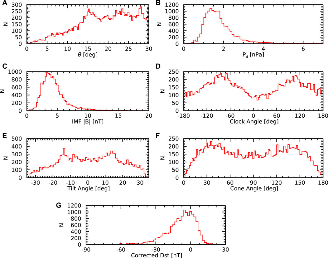
Figure 2. Histograms of the parameters associated with individual magnetopause crossings. (A) Crossing angle θ, which is the angle between the positional vector of the crossing and the x-axis. (B) Solar wind dynamic pressure. (C) Interplanetary magnetic field magnitude. (D) Clock angle. (E) Tilt Angle. (F) Cone angle. (G) Corrected Dst index.

Figure 2A shows a histogram of the crossing angle θ values. Due to geometrical reasons, most magnetopause crossings are at larger values of θ (note that the area of magnetopause at a given value of θ scales roughly as ∝ sin θ). The distribution of the solar wind dynamic pressure is depicted in Figure 2B. It can be seen that the solar wind dynamic pressure values are mostly between about 1 and 3 nPa. However, the distribution has a rather significant tail, with the dynamic pressure occasionally being as high as 7 nPa. Similarly, the distribution of IMF magnitudes depicted in Figure 2C reveals that most magnetopause crossings are observed at IMF magnitudes between about 2 and 8 nT, consistent with the long-term solar wind properties. Figure 2D shows the distribution of the IMF clock angle [the angle between the GSM z-axis and the projection of the IMF vector onto the GSM Y-Z plane, arctan(B_y/B_z)]. The two peaks at ± 90° are formed due to the typically rather low value of IMF B_z. Figure 2E depicts the distribution of the tilt angle (the angle between the Earth’s magnetic dipole axis and the GSM z-axis). The range of the dipole tilt angle is given by the sum of the Earth’s dipole tilt with respect to the rotational axis (about 11°) and the inclination of the Earth’s rotational axis with respect to the ecliptic (about 23.5°). The extreme values of the tilt angle are rather rare, as they require a specific combination of the Earth’s rotation and season. Figure 2F shows the distribution of the cone angle (the angle between the IMF and the velocity of the solar wind). The two maxima at about 45° and 135° are in line with the Parker spiral theory and the Earth-Sun distance of 1 AU. Finally, Figure 2G shows a histogram of corrected Dst index at the times of the magnetopause crossings. The corrected Dst index is essentially the traditional Dst index with the contribution of the magnetopause currents subtracted, corresponding thus better to the magnitude of the ring current (Burton et al., 1975).

3 Neural network models

Compared to a predefined empirical model formulation and subsequent fitting of free parameters to observed magnetopause crossings, artificial neural networks offer a more general approach. This approach allows for optimal matching of desired outputs with respective inputs contained in the training data set. The idea is inspired by real biological neurons. A multi-layer feed-forward neural network configuration (Wythoff, 1993) we use consists of the first (input) layer of neurons, several interim (hidden) layers, and the last (output) layers. The inputs are the magnetopause crossing angle θ and individual parameters controlling the magnetopause crossing distance. The output is a single number corresponding to the magnetopause radial distance. During the learning process, the neural network configuration is adjusted using a training data set in such a way that the predicted (model) radial distances of magnetopause crossings match the observed radial distances as closely as possible. The degree of this match is quantified using a loss function; a common choice, and the one we employ, is the mean square error. Adjusting the neural network configuration thus in fact corresponds to a fitting process. However, the fitting function is given by the neural network itself, allowing an extremely large range of nonlinear dependences to be included, and thus effectively removing the limitation of a prescribed empirical fitting function.

An important aspect of neural network configuration is that each neuron is connected to all neurons in the subsequent layer, and each connection has a distinct weight. The output of a given neuron is calculated as a weighted sum of its inputs, to which a bias term is added. Subsequently, an activation function is applied to this sum. The weights of the connections between individual neurons represent their significance. These values are adjusted during the neural network training process (McCulloch and Pitts, 1943; Svozil et al., 1997). This adjustment can be performed using a backpropagation learning algorithm, where the error is progressively transferred from the output layer to the input layer, and the connection weights are iteratively adjusted (Haykin, 1998).

It is not desirable to use the same data set for training and testing the neural network. The reason is that, if the same data set is used, the neural network may overfit and focus on features that are not representative of the entire data set. Therefore, the data set is randomly divided into two distinct parts: a training data set and a testing data set. In our case, 80% and 20% of the data are allocated to these data sets, respectively. The exact neural network configuration, including the activation functions, number of layers, and the number of neurons in each layer, can be somewhat arbitrary. After numerous trials with various configurations, we found that, in our case, the specific configuration used has only a rather marginal effect on the overall performance. We note, however, that the situation of too few neurons/layers should be avoided as it does not allow to describe a sufficiently general dependence of the magnetopause location on the control parameters, limiting the possible outcomes of the model. On the other hand, the situation of too many neurons/layers should be avoided as well, as it may result in overfitting, i.e., in the neural network model nit-picking irrelevant rare features, outliers, etc. We eventually settled on using hyperbolic tangent as an activation function and two hidden layers comprising 30 and 15 neurons, respectively. The neural network optimization is done using the adaptive moment estimation algorithm, iterating until effective convergence is achieved.

Two different magnetopause models are constructed based on neural networks. The first model is developed using three input parameters: magnetopause crossing angle θ, solar wind dynamic pressure, and IMF B_z. These parameters are identical to those used in the popular model by Shue et al. (1997), allowing for a direct comparison of the model performance. The second model does not expect an explicit dependence on IMF B_z, but rather adds five other parameters influencing the magnetopause location: IMF magnitude, clock angle, cone angle, tilt angle, and the corrected Dst index. This model thus has a total of seven input parameters, replacing the magnetopause location dependence on IMF B_z with a dependence on the IMF clock angle and magnitude. We note that parameterizing the IMF vector by its magnitude and the two angles (clock angle and cone angle) is desirable, as it ensures relative independence of the parameters.

Input values are normalized using arctan before being fed into the neural network, ensuring uniform range and a central value of zero. However, it is possible to significantly improve the neural network performance and ensure its adherence to the physical symmetries involved by a pre-transformation of the input variables. Due to the long tail of the solar wind dynamic pressure distribution, its logarithm is considered instead of the actual value. For symmetry arguments, the sine of the cone angle is used in place of the cone angle itself, the square of the sine of its half is used in place of the clock angle, and the absolute value of the tilt angle is used instead of the tilt angle.

4 Model performance and dependences

The performance of the first neural network model based exclusively on the magnetopause crossing angle θ, solar wind dynamic pressure, and IMF B_z is evaluated and compared with the performance of the Shue et al. (1997) model in Figure 3. Figure 3A shows the magnetopause radial distances predicted by the neural network model as a function of the observed magnetopause radial distances. Each red point corresponds to a single magnetopause crossing and the black line shows a one-to-one dependence. It can be seen that the model and observed magnetopause distances are well correlated (Pearson’s correlation coefficient of about 0.74), with the model tendency to underpredict the radial distances for very distant magnetopause crossings. Note that a few magnetopause crossings at very extreme distances are not shown in this plot due to the range of axes used; they are, nevertheless, included in the calculation of correlation coefficients and standard deviations. Figure 3B uses the same representation, but employing the Shue et al. (1997) in place of the neural network model. Essentially the same correlation coefficient is obtained (0.76), with the model tendency to underpredict the magnetopause radial distances overall, but in particular for distant magnetopause crossings. Histogram of the differences between the observed magnetopause radial distances and the radial distances predicted by the neural network and Shue et al. (1997) models are depicted in Figure 3C by the red and blue lines, respectively. The red and blue vertical lines show the median values of the respective distributions. The histogram of differences corresponding to the neural network model appears somewhat narrower (albeit the standard deviations are quite the same, 0.67 R_E vs. 0.65 R_E) and it is better centered at zero (median value of −0.1 R_E vs. 0.5 R_E). This is confirmed by Figure 3D, which uses the same representation to depict the histogram of ratios of observed and model magnetopause radial distances (standard deviation of 0.05 vs. 0.06, median value of 0.99 vs. 1.04).

Figure 3

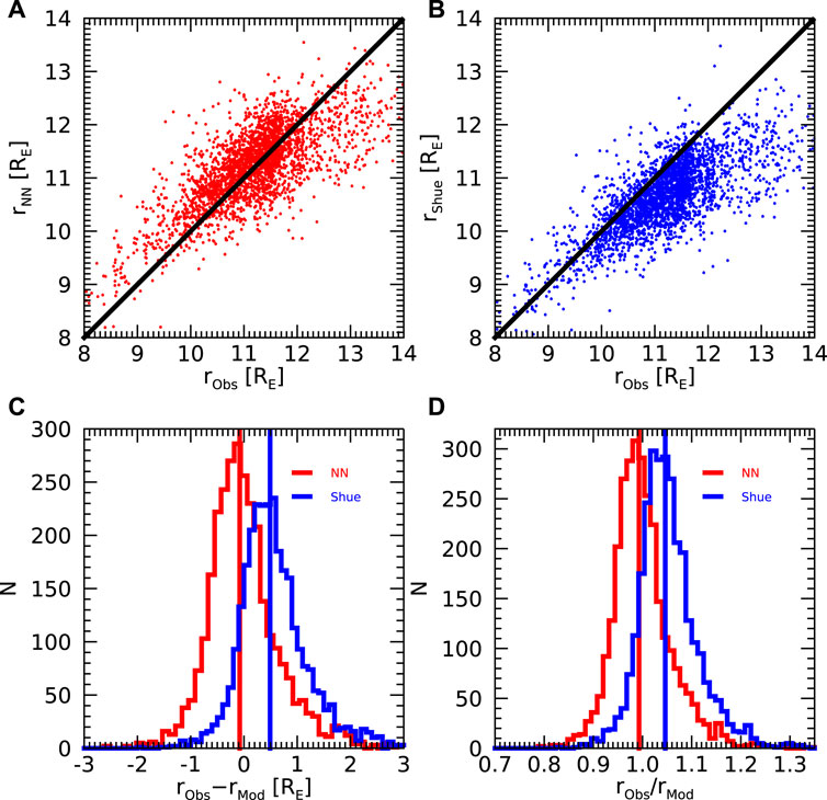
Figure 3. Comparison of the performance of the neural network model based on the three main parameters (θ, dynamic pressure, and IMF B_z) with the Shue et al. (1997) model. (A) Magnetopause distances predicted by the neural network model vs. observed magnetopause distances. The black line shows the 1:1 dependence. (B) The same as (A), but for the Shue et al. (1997) magnetopause model. (C) Histogram of differences between observed and model magnetopause distances. The results obtained for the neural network model and the Shue et al. (1997) model are shown by the red and blue lines, respectively. The vertical color lines show the respective median values. (D) The same as (C), but for the ratios of observed to model magnetopause distances.

The results obtained for the second neural network model based on all the seven input parameters (magnetopause crossing angle θ, solar wind dynamic pressure, IMF magnitude, clock angle, cone angle, tilt angle, and corrected Dst index) are depicted in Figure 4. The panel format used is the same as in Figure 3. Figure 4A shows the magnetopause radial distances predicted by the neural network model as a function of the observed magnetopause distances, with each red dot representing a single magnetopause crossing. The black line again corresponds to the one-to-one dependence. A reasonable agreement between the model and the observations can be seen (correlation coefficient of about 0.78), with only a slight tendency of the model to underpredict the larger radial distances. Figures 4B, C show, respectively, the differences and ratios of observed and model magnetopause radial distances. It can be seen that, on average, the model predictions well correspond to the observations, with nearly no systematic bias (median value of differences −0.1 R_E, median value of ratios 0.99). Moreover, the distributions of differences/ratios are slightly narrower than those in Figure 3. The corresponding standard deviations are 0.61 R_E and 0.05, respectively.

Figure 4

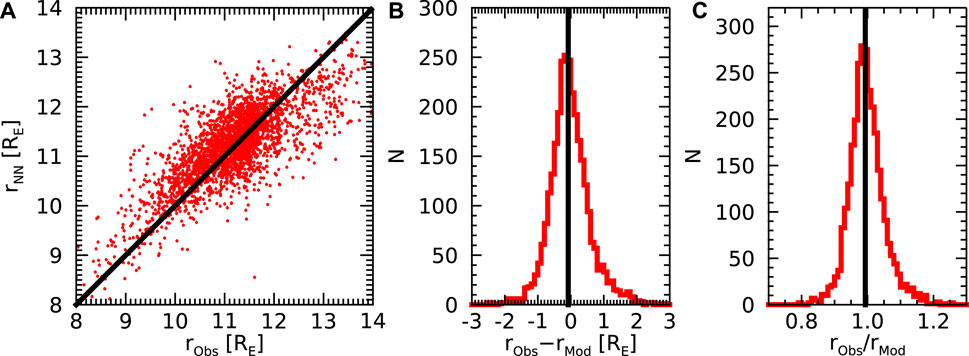
Figure 4. (A) Performance of the neural network model based on seven parameters (θ, dynamic pressure, IMF magnitude, clock angle, cone angle, tilt angle, corrected Dst index). (A) Magnetopause distances predicted by the neural network model vs. observed magnetopause distances. The black line shows the 1:1 dependence. (B) Histogram of differences between observed and model magnetopause distances. The vertical line shows the respective median value. (C) The same as (B), but for the ratios of observed to model magnetopause distances.

In order to better understand the uncertainty of the neural network model predictions and the dependence on individual parameters, the neural network model based on the seven parameters was trained not a single time but a hundred times. Each time, the training set was randomly selected so that it was different across individual training instances, resulting in slightly different models providing slightly different magnetopause distance predictions. This allows us to determine the mean model prediction and its standard deviation (calculated over the set of hundred neural network models, evaluated for given input parameters). The results obtained for the subsolar magnetopause distance are depicted in Figure 5. Each panel corresponds to a dependence on a single input parameter, with the remaining parameters fixed at their median/characteristic values. The black curves show the average model predictions, while the red and green curves correspond to the average value ±1 standard deviation.

Figure 5

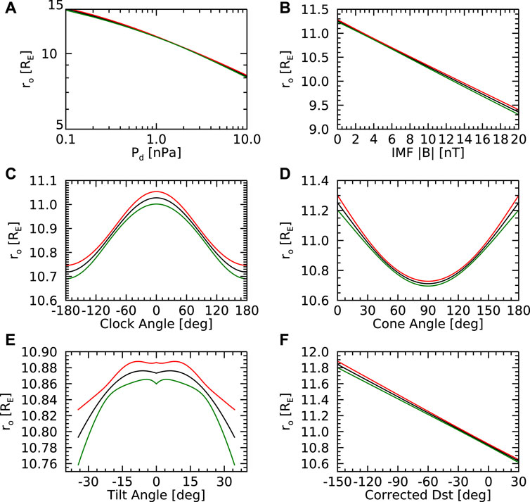
Figure 5. Magnetopause distance in the subsolar point predicted by neural network model as a function of (A) Solar wind dynamic pressure. (B) IMF magnitude. (C) Clock angle. (D) Cone angle. (E) Tilt angle. (F) Corrected Dst index. The three curves plotted in individual panels correspond to the mean dependence and ±1 standard deviation confidence interval.

Figure 5A shows the subsolar magnetopause distance r₀ as a function of the solar wind dynamic pressure p_d. A systematic monotonic decrease of the radial distance with increasing dynamic pressure can be seen, as expected. Given the logarithmic scales of the plot, a straight line would indicate the expected power law dependence $(R_0\propto p_d^{\alpha })$. However, the slope of the dependence becomes slightly steeper for larger dynamic pressures. The power law dependence at low dynamic pressures would have the exponent of α ≈ − 1/9.0, while at high dynamic pressures α ≈ − 1/6.2. This variation in the power law index with the dynamic pressure may be attributed to the influence of the limited spacecraft apogee, as demonstrated by Němeček et al. (2020). However, it might also suggest that a single, constant power law index is not universally applicable. Regardless, the obtained values are roughly in line with the −1/6 value stemming from a simple pressure balance of the dynamic and magnetic field pressures, assuming the magnetic field to decrease as a cube of the radial distance, and with the −1/6.6 value reported by Shue et al. (1997). Note, however, that the dependence in Figure 5A is purely data-driven, with no a priori assumptions.

Figure 5B reveals a systematic monotonic decrease of the subsolar magnetopause distance with the IMF magnitude. This is apparently in line with the results obtained by Li et al. (2023), suggesting that the solar wind/magnetosheath magnetic field pressure non-negligibly contributes to the pressure balance, as accounted for in some newer empirical models (Lin et al., 2010). The subsolar magnetopause distance dependence on the clock angle depicted in Figure 5C is somewhat more complicated and noticeably weaker. It is, by definition, symmetric around zero (recall that the square of the sine of half of the cone angle is used as the neural network input). The subsolar magnetopause distance is found to be maximal for zero clock angles (corresponding to the northward IMF) and minimal for clock angles of ±180° (corresponding to the southward IMF). This trend is well in line with former empirical models (e.g., Shue et al., 1997). The cone angle effect on the subsolar magnetopause distance investigated in Figure 5D is of a similar magnitude. The magnetopause is found at larger radial distances at the times of cone angle close to 0° and 180°, i.e., at the times of the radial IMF, in agreement with former studies (Dušík et al., 2010; Samsonov et al., 2012).

The tilt angle effect analyzed in Figure 5E is very weak. The small dip/peak observed at a tilt angle equal to zero is an artifact given by the predefined symmetry (recall that the absolute value of the tilt angle is used as the neural network input), and—given its magnitude being smaller than the standard deviation—can be quite ignored. Figure 5F further shows that subsolar magnetopause distance tends to be larger at the times of large negative corrected Dst index. This suggests the importance of the ring current and the corresponding magnetic field on the magnetospheric side of the dayside magnetopause (Machková et al., 2019). We note that the corrected Dst index is governed by the solar wind parameters and their short-term history, particularly by the clock angle (IMF B_z). At times of southward IMF, the clock angle effect results in smaller magnetopause distances. However, simultaneously, the Dst index is typically more negative, tending to increase the magnetopause distances. The two effects may thus partially cancel each other.

Having demonstrated the reasonable performance of our purely data-driven magnetopause model based on the neural network, we further try to understand why all the models (albeit arguably better and better) do not seem to improve too much. There seems to be an intrinsic limitation of their accuracy, no matter how complicated these models become and how many parameters possibly controlling the magnetopause location are considered. We argue that this limitation stems from the inaccurately known solar wind parameters, most importantly the solar wind dynamic pressure (as the main factor controlling the magnetopause location). These are typically not measured just upstream the Earth, but rather close to the L1 point and then propagated to Earth (i.e., essentially just time delayed). We further demonstrate that this propagation may result in a considerable inaccuracy in the solar wind dynamic pressure, eventually limiting the accuracy of the magnetopause model predictions.

A combination of the Wind spacecraft data close to the L1 point, OMNI data, and the THEMIS B and THEMIS C data just upstream the bow shock is used for this purpose. Altogether, as many as 8,268,027 THEMIS measurements of the solar wind dynamic pressure with a time resolution of 3 s are used for this purpose. Corresponding solar wind dynamic pressure value based on the measurements close to the L1 point is attributed to each data point using our two-step propagation routine as well as using the OMNI data set. Histograms of the ratios of these propagated solar wind dynamic pressures (p_sw) and the solar wind dynamic pressures observed by THEMIS (p_THEMIS) are depicted in Figure 6A. The red line corresponds to the OMNI data propagation, while the blue line corresponds to our two-step propagation of the Wind data. In an optimal situation, a very narrow peak centered at one would be obtained. However, this is not the case. The distribution is rather broad and, moreover, there appears to be a systematic shift towards larger pressure ratios, corresponding to a systematic difference between THEMIS and Wind measurements. This systematic difference may be partly due to some THEMIS data being measured in the foreshock region, where the solar wind is already somewhat decelerated (Urbář et al., 2019), and partly due to the internal inaccuracies of the instruments used, as is the case with the Magnetospheric Multiscale (MMS) mission, for example (Roberts et al., 2021). Nevertheless, the broadness of the distribution is the issue.

Figure 6

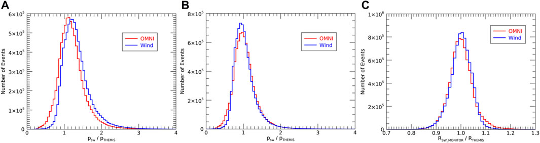
Figure 6. (A) Histogram of the ratio of the solar wind dynamic pressure propagated from the Lagrange L1 point and the solar wind dynamic pressure measured by the THEMIS spacecraft just upstream of the bow shock. The red histogram shows the results obtained for the propagation used in the OMNI data set, while the blue line shows the results obtained for our own propagation routine of the Wind spacecraft data. (B) The same as (A), but the respective ratios are multiplied by a constant to ensure their median is equal to one, accounting for systematic differences between the measurements of individual spacecraft instruments. (C) Histogram of the ratios of magnetopause radial distances corresponding to (B), assuming that the power law dependence of the magnetopause radial distance on the dynamic pressure with an exponent of −1/6 $(R\propto p_d^{-1/6})$.

The systematic difference in the observed dynamic pressures can be easily accounted for, e.g., through a multiplication by a factor which ensures that the median of the distribution is equal to unity. This is done in Figure 6B. However, the issue of the widths of the distributions (standard deviations of about 0.3), indicating an intrinsic inaccuracy in the propagation itself, remains. This inaccuracy can be recalculated to the corresponding inaccuracy of the magnetopause location, assuming that the magnetopause radial distance depends on the solar wind dynamic pressure as $R\propto p_d^{-1/6}$. The ratios of the solar wind dynamic pressures from Figure 6B are then converted to the ratios of the magnetopause radial distances in Figure 6C. Distributions with standard deviations of about 0.050 and 0.045 are obtained for the OMNI and our two-step propagation of Wind measurements, respectively. These effectively represent the accuracy limit of magnetopause models stemming from the inaccuracy in the solar wind dynamic pressure propagation from the L1 point. They can be directly compared with Figures 3D, 4C which depict the ratios of the observed to model magnetopause distances.

5 Discussion

A large data set of subsolar magnetopause crossings compiled using data measured by several different spacecraft has been used. Being close to the subsolar point, the crossing locations are virtually unaffected by the cusp indentations, and, moreover their radial distances are comparatively low to suffer from the sampling bias due to the limited spacecraft apogee.

The primary benefit of the neural network modeling approach employed is that it nearly eliminates the need for a priori assumptions regarding the model formulation and the magnetopause location dependence on individual parameters. Additionally, the flexibility of the neural network model makes it easier to extend the model by including other possible controlling parameters.

However, two initial decisions limiting the model generality are still necessary. The first decision concerns the choice of model parameters and their possible pre-normalization to respect the symmetries involved. In our study, we use a single value to describe the magnetopause crossing direction, assuming its symmetricity around the direction of the incoming solar wind. Although this assumption is well justified by the fact that only near-subsolar region is studied, it may be possibly desirable to release this constraint in further studies. Moreover, the proper consideration of the symmetries based on the physical insight into the problem improves the model outcome considerably. This concerns, in particular, the parameterization of the IMF, where the used approach of the IMF magnitude and properly transformed clock and cone angles is superior to, e.g., considering individual Cartesian coordinates of IMF. The second, less limiting, decision needed are the technical details of the neural network configuration used. Many different configurations, parameter normalizations, and neuron activation functions have been tried. Nevertheless, it turns out that, as long as these are not very extreme, they have only a marginal effect on the neural network performance.

Two different neural network models are constructed. The first of them uses a simple parameterization exactly following the traditional Shue et al. (1997) model to allow for a direct comparison. This revealed that the neural network model performance is comparable to the Shue et al. (1997) model, demonstrating the feasibility of the neural network approach for the magnetopause model formulation. The second neural network model developed uses as many as seven different parameters and slightly outperforms the other models. However, its main aim is to show that the employed neural network approach can be used to isolate the effects of individual parameters, and to eventually obtain the respective data-driven magnetopause distance dependences. The obtained effects of individual parameters are in line with former studies. This concerns the dependence on the solar wind dynamic pressure and IMF B_z (e.g., Shue et al., 1997), cone angle (Dušík et al., 2010; Samsonov et al., 2012), IMF magnitude (Lin et al., 2010; Li et al., 2023), and corrected Dst index (Machková et al., 2019). The effect of the tilt angle appears to be very weak, which is perhaps due to our data set being limited to the vicinity of the subsolar point, avoiding the cusp regions (Safrankova and Dusik, 2005).

Finally, we focus on the evaluation of intrinsic limitations of the magnetopause location predictions due to the inaccuracy of the upstream solar wind dynamic pressure propagated from the L1 point. A comparison of the solar wind dynamic pressure measured by the THEMIS spacecraft in the solar wind just upstream the bow shock with the corresponding dynamic pressure propagated from the L1 point reveals that, albeit the two values generally reasonably agree, the distribution of their ratios is rather broad, with a standard deviation of about 0.3. Assuming that the magnetopause distance depends on the solar wind dynamic pressure roughly as $R\propto p_d^{-1/6}$, we can directly translate this to the uncertainty of about 5% in the magnetopause distance. This provides us with the accuracy limit achievable by the magnetopause models, which is not possible to surpass unless better solar wind dynamic pressure data are available. We note that the real accuracy limit is even more severe, as additional sources of error are clearly present. The content of alphas and heavier particles in the solar wind is rarely properly considered, and the propagation of other solar wind parameters—although their effects on the magnetopause location are weaker—suffers from the same problems. Various solar wind structures present at L1 may evolve during their propagation to Earth or they may actually miss Earth completely. Moreover, the time history of the magnetospheric system and the dynamic motion of the magnetopause are not considered within the static approximation employed by empirical models. Consequently, it appears that the recent empirical magnetopause models eventually approach the theoretical accuracy threshold. In this sense, a development of more accurate magnetopause models may not be possible. On the other hand, it is still possible to learn about important physical processes and dependences involved using a statistical approach, where the inaccuracies of the solar wind parameters eventually average out.

6 Conclusion

We used about 15,000 subsolar magnetopause crossings identified in the THEMIS A-E, Magion 4, Geotail, and Interball satellite data to investigate the possibility of modeling the magnetopause radial distance using a neural network. Furthermore, the intrinsic inaccuracy of magnetopause models due to the solar wind parameter propagation from the L1 point was demonstrated.

Two magnetopause models based on the neural network approach were constructed. The first model has only three parameters (magnetopause crossing angle θ, solar wind dynamic pressure, IMF B_z), mimicking closely the traditional Shue et al. (1997) empirical model. It was used to demonstrate the suitability of the approach, achieving the accuracy comparable with the Shue et al. (1997) model without the need of any a priori assumptions on the model formulation. The second model has seven parameters (magnetopause crossing angle θ, solar wind dynamic pressure, IMF magnitude, clock angle, cone angle, tilt angle, and corrected Dst index). It resulted in a slightly better accuracy. The analysis of the predicted subsolar magnetopause distance as a function of individual controlling parameters allowed us to demonstrate that the respective dependences are indeed quite reasonable and correspond to the expectations, albeit purely data-driven, with no a priori assumptions.

Finally, we show that the accuracy of predicting the magnetopause location is limited by our insufficient information about the upstream solar wind parameters. These are typically propagated from the L1 point. However, we show that the real upstream solar wind parameters may be quite different. Consequently, even a perfect model would not in principle predict the magnetopause location precisely, due to the inaccuracy of the input parameters. We show that this accuracy threshold is rather approached by recent empirical models.

Data availability statement

Publicly available datasets were analyzed in this study. This data can be found here: https://cdaweb.gsfc.nasa.gov/.

Author contributions

MA: Conceptualization, Data curation, Formal Analysis, Investigation, Methodology, Software, Validation, Visualization, Writing–original draft, Writing–review and editing. FN: Conceptualization, Data curation, Formal Analysis, Funding acquisition, Investigation, Methodology, Project administration, Resources, Software, Supervision, Validation, Visualization, Writing–original draft, Writing–review and editing. GP: Conceptualization, Data curation, Formal Analysis, Methodology, Software, Validation, Writing–original draft, Writing–review and editing. ZN: Formal Analysis, Funding acquisition, Investigation, Methodology, Resources, Validation, Writing–original draft, Writing–review and editing. JaS: Formal Analysis, Funding acquisition, Investigation, Methodology, Resources, Validation, Writing–original draft, Writing–review and editing. KG: Data curation, Software, Writing–original draft, Writing–review and editing. JiS: Data curation, Software, Writing–original draft, Writing–review and editing. T-CT: Data curation, Formal Analysis, Software, Validation, Writing–original draft, Writing–review and editing.

Funding

The authors declare that financial support was received for the research, authorship, and/or publication of this article. The work was supported by the Czech Science Foundation (GACR) under Contract 21-26463S.

Acknowledgments

The authors thank all the spacecraft teams for the magnetic field and plasma data.

Conflict of interest

The authors declare that the research was conducted in the absence of any commercial or financial relationships that could be construed as a potential conflict of interest.

Publisher’s note

All claims expressed in this article are solely those of the authors and do not necessarily represent those of their affiliated organizations, or those of the publisher, the editors and the reviewers. Any product that may be evaluated in this article, or claim that may be made by its manufacturer, is not guaranteed or endorsed by the publisher.

References

Aghabozorgi, M., Němec, F., Pi, G., Němeček, Z., Šafránková, J., Grygorov, K., et al. (2023). Interplanetary magnetic field b_y controls the magnetopause location. J. Geophys. Res. 128. doi:10.1029/2023JA031303

CrossRef Full Text | Google Scholar

Boardsen, S. A., Eastman, T. E., Sotirelis, T., and Green, J. L. (2000). An empirical model of the high-latitude magnetopause. J. Geophys. Res. 105, 23193–23219. doi:10.1029/1998JA000143

CrossRef Full Text | Google Scholar

Bonde, R. E. F., Lopez, R. E., and Wang, J. Y. (2018). The effect of IMF fluctuations on the subsolar magnetopause position: a study using a global MHD model. J. Geophys. Res. Space Phys. 123, 2598–2604. doi:10.1002/2018JA025203

CrossRef Full Text | Google Scholar

Burton, R. K., McPherron, R., and Russell, C. (1975). An empirical relationship between interplanetary conditions and Dst. J. Geophys. Res. 80, 4204–4214. doi:10.1029/JA080i031p04204

CrossRef Full Text | Google Scholar

Cahill, L. J., and Amazeen, P. G. (1963). The boundary of the geomagnetic field. J. Geophys. Res. 68, 1835–1843. doi:10.1029/JZ068i007p01835

CrossRef Full Text | Google Scholar

Case, N. A., and Wild, J. A. (2013). The location of the Earth’s magnetopause: a comparison of modeled position and in situ Cluster data. J. Geophys. Res. Space Phys. 118, 6127–6135. doi:10.1002/jgra.50572

CrossRef Full Text | Google Scholar

Dušík, Š., Granko, G., Šafránková, J., Němeček, Z., and Jelínek, K. (2010). IMF cone angle control of the magnetopause location: statistical study. Geophys. Res. Lett. 37. doi:10.1029/2010GL044965

CrossRef Full Text | Google Scholar

Fairfield, D. H. (1971). Average and unusual locations of the Earth’s magnetopause and bow shock. J. Geophys. Res. 76, 6700–6716. doi:10.1029/JA076i028p06700

CrossRef Full Text | Google Scholar

Formisano, V., Domingo, V., and Wenzel, K.-P. (1979). The three-dimensional shape of the magnetopause. Planet. Space Sci. 27, 1137–1149. doi:10.1016/0032-0633(79)90134-X

CrossRef Full Text | Google Scholar

Grygorov, K., Němeček, Z., Šafránková, J., Šimůnek, J., and Gutynska, O. (2022). Storm-time magnetopause: pressure balance. J. Geophys. Res. Space Phys. 127. doi:10.1029/2022JA030803

CrossRef Full Text | Google Scholar

Haaland, S., Hasegawa, H., Paschmann, G., Sonnerup, B., and Dunlop, M. (2021). 20 years of Cluster observations: the magnetopause. J. Geophys. Res. Space Phys. 126. doi:10.1029/2021JA029362

CrossRef Full Text | Google Scholar

Haykin, S. (1998) Neural networks: a comprehensive foundation. Prentice Hall PTR.

Google Scholar

Lavraud, B., Larroque, E., Budnik, E., Génot, V., B, J. E., Dunlop, M. W., et al. (2013). Asymmetry of magnetosheath flows and magnetopause shape during low Alfvén Mach number solar wind. J. Geophys. Res. 118, 1089–1100. doi:10.1002/jgra.50145

CrossRef Full Text | Google Scholar

Li, S., Sun, Y. Y., and Chen, C.-H. (2023). An interpretable machine learning procedure which unravels hidden interplanetary drivers of the low latitude dayside magnetopause. Space weather. 21, e2022SW003391. doi:10.1029/2022SW003391

CrossRef Full Text | Google Scholar

Lin, R. L., Zhang, X. X., Liu, S. Q., Wang, Y. L., and Gong, J. C. (2010). A three-dimensional asymmetric magnetopause model. J. Geophys. Res. Space Phys. 115. doi:10.1029/2009JA014235

CrossRef Full Text | Google Scholar

Liu, Z. Q., Lu, J. Y., Wang, C., Kabin, K., Zhao, J. S., Wang, M., et al. (2015). A three-dimensional high Mach number asymmetric magnetopause model from global MHD simulation. J. Geophys. Res. 120, 5645–5666. doi:10.1002/2014JA020961

CrossRef Full Text | Google Scholar

Lu, J. Y., Liu, Z. Q., Kabin, K., Jing, H., Zhao, M. X., and Wang, Y. (2013). The IMF dependence of the magnetopause from global MHD simulations. J. Geophys. Res. Space Phys. 118, 3113–3125. doi:10.1002/jgra.50324

CrossRef Full Text | Google Scholar

Machková, A., Němec, F., Němeček, Z., and Šafránková, J. (2019). On the influence of the Earth’s magnetic dipole eccentricity and magnetospheric ring current on the magnetopause location. J. Geophys. Res. Space Phys. 124, 905–914. doi:10.1029/2018JA026070

CrossRef Full Text | Google Scholar

McCulloch, W. S., and Pitts, W. A. (1943). A logical calculus of the ideas immanent in nervous activity. Bull. Math. biophysics 5, 115–133. doi:10.1007/BF02478259

CrossRef Full Text | Google Scholar

Merka, J., Szabo, A., Šafránková, J., and Němeček, Z. (2003). Earth’s bow shock and magnetopause in the case of a field-aligned upstream flow: observation and model comparison. J. Geophys. Res. Space Phys. 108. doi:10.1029/2002JA009697

CrossRef Full Text | Google Scholar

Němeček, Z., Šafránková, J., Grygorov, K., Mokrý, A., Pi, G., Aghabozorgi Nafchi, M., et al. (2023). Extremely distant magnetopause locations caused by magnetosheath jets. Geophys. Res. Lett. 50. doi:10.1029/2023GL106131

CrossRef Full Text | Google Scholar

Němeček, Z., Šafránková, J., Lopez, R. E., Dušík, Š., Nouzák, L., Přech, L., et al. (2016). Solar cycle variations of magnetopause locations. Adv. Space Res. 58, 240–248. doi:10.1016/j.asr.2015.10.012

CrossRef Full Text | Google Scholar

Němeček, Z., Šafránková, J., and Šimůnek, J. (2020). An examination of the magnetopause position and shape based upon new observations. Dayside Magnetos. Interact. 248, 135–151. doi:10.1002/9781119509592.ch8

CrossRef Full Text | Google Scholar

Park, J., Shue, J., Kim, K., Pi, G., Němeček, Z., and Šafránková, J. (2016). Global expansion of the dayside magnetopause for long-duration radial IMF events: statistical study on GOES observations. J. Geophys. Res. Space Phys. 121, 6480–6492. doi:10.1002/2016JA022772

CrossRef Full Text | Google Scholar

Petrinec, S. M., and Russell, C. T. (1996). Near-Earth magnetotail shape and size as determined from the magnetopause flaring angle. J. Geophys. Res. 101, 137–152. doi:10.1029/95JA02834

CrossRef Full Text | Google Scholar

Roberts, O. W., Nakamura, R., Coffey, V. N., Gershman, D. J., Volwerk, M., and Varsani, A. (2021). A study of the solar wind ion and electron measurements from the magnetospheric multiscale mission's fast plasma investigation. J. Geophys. Res.: Space Phys. 126, e2021JA029784. doi:10.1029/2021JA029784

CrossRef Full Text | Google Scholar

Roelof, E. C., and Sibeck, D. G. (1993). Magnetopause shape as a bivariate function of interplanetary magnetic field B_z and solar wind dynamic pressure. J. Geophys. Res. Space Phys. 98 (21), 421–21. doi:10.1029/93JA02362

CrossRef Full Text | Google Scholar

Šafránková, J., Dušík, Š., and Němeček, Z. (2005). The shape and location of the high-latitude magnetopause. Adv. Space Res. 36, 1934–1939. doi:10.1016/j.asr.2004.05.009

CrossRef Full Text | Google Scholar

Šafránková, J., Němeček, Z., Dušík, Š., Přech, L., Sibeck, D. G., and Borodkova, N. N. (2002). The magnetopause shape and location: a comparison of the Interball and Geotail observations with models. Ann. Geophys. 20, 301–309. doi:10.5194/angeo-20-301-2002

CrossRef Full Text | Google Scholar

Samsonov, A. A., Němeček, Z., Šafránková, J., and Jelínek, K. (2012). Why does the subsolar magnetopause move sunward for radial interplanetary magnetic field? J. Geophys. Res. Space Phys. 117. doi:10.1029/2011JA017429

CrossRef Full Text | Google Scholar

Shue, J. H., Chao, J. K., Fu, H. C., Russell, C. T., Song, P., Khurana, K. K., et al. (1997). A new functional form to study the solar wind control of the magnetopause size and shape. J. Geophys. Res. Space Phys. 102, 9497–9511. doi:10.1029/97JA00196

CrossRef Full Text | Google Scholar

Sibeck, D. G., Lopez, R. E., and Roelof, E. C. (1991). Solar wind control of the magnetopause shape, location, and motion. J. Geophys. Res. 96, 5489–5495. doi:10.1029/90JA02464

CrossRef Full Text | Google Scholar

Svozil, D., Kvasnicka, V., and Pospichal, J. (1997). Introduction to multi-layer feed-forward neural networks. Chemom. intelligent laboratory Syst. 39, 43–62. doi:10.1016/S0169-7439(97)00061-0

CrossRef Full Text | Google Scholar

Urbář, J., Němeček, Z., Šafránková, J., and Přech, L. (2019). Solar wind proton deceleration in front of the terrestrial bow shock. J. Geophys. Res.: Space Phys. 124 (8), 6553–6565. doi:10.1029/2019JA026734

CrossRef Full Text | Google Scholar

Verigin, M. I., Kotova, G. A., Bezrukikh, V. V., Zastenker, G. N., and Nikolaeva, N. (2009). Analytical model of the near-Earth magnetopause according to the data of the Prognoz and Interball satellite data. Geomagnetism Aeronomy 49, 1176–1181. doi:10.1134/S0016793209080283

CrossRef Full Text | Google Scholar

Wang, Y., Sibeck, D. G., Merka, J., Boardsen, S. A., Karmabadi, H., Sipes, T. B., et al. (2013). A new three-dimensional magnetopause model with a support vector regression machine and a large database of multiple spacecraft observations. J. Geophys. Res. Space Phys. 118, 2173–2184. doi:10.1002/jgra.50226

CrossRef Full Text | Google Scholar

Wythoff, B. J. (1993). Backpropagation neural networks: a tutorial. Chemom. Intelligent Laboratory Syst. 18, 115–155. doi:10.1016/0169-7439(93)80052-J

CrossRef Full Text | Google Scholar