Probing turbulence in solar flares from SDO/AIA emission lines

Multiple pieces of evidence have revealed the important role of turbulence in physical processes in solar eruptions, from particle acceleration to the suppression of conductive cooling. Radio observations of density variation have established a Kolmogorov-like spectrum for solar wind density disturbance. Close to the Sun, measurements from extreme ultraviolet (EUV) bands have been used to examine turbulence in the solar atmosphere. The Atmospheric Imaging Assembly onboard the Solar Dynamics Observatory (SDO/AIA) has been frequently used for diagnosing plasma properties due to its complex coverage of temperature response. We compute structure functions (SFs) using SDO/AIA emission measurements for two example of plasma sheets. With the relationship of v ∼ b ∼ δn and $\delta I\sim \delta {(n_0+\delta n)}^2\sim \delta n$ (v, b, δn, and δI are turbulent velocity, magnetic field, number density, and intensity, respectively, and n₀ is the background density), SFs of δI can be regarded as a proxy for those of the turbulent v and b fields in the plasma sheet. We show that by properly accounting for the radial dependence of the emission line intensity, an SF method is capable of probing the presence of turbulence from SDO/AIA emission lines. Compared to in situ observations, performing SFs on EUV emissions is advantageous in studying turbulence behavior in the wave-vector space, and it opens a new window for investigating turbulence from massive SDO/AIA observations.

1 Introduction

Turbulent flows are an inevitable result of the high Reynolds number in the solar corona (Priest, 2014; Emslie and Bradshaw, 2022), and efforts to characterize turbulence in solar plasma have been made over decades (Antonucci, 1989; Rosa et al., 1998; Effenberger and Petrosian, 2018; Kumar and Choudhary, 2023). Turbulence has a great impact on physical processes in solar eruptions (Vlahos and Isliker, 2023), such as particle acceleration (Li et al., 2022; Wu et al., 2023), the suppression of thermal conduction (Jiang et al., 2006; Bian et al., 2016a), the extension of flare heating (Ashfield and Longcope, 2023), and the enhancement of magnetic reconnection rate (Huang and Bhattacharjee, 2016; Wang et al., 2023). The most quasi-direct observations that reveal the presence of turbulence in solar flaring structures are via spectrometry (Antonucci et al., 1982; del Zanna et al., 2006; Milligan, 2011; Jeffrey et al., 2016; Polito et al., 2018; Kerr, 2022; Kerr, 2023). The spectroscopic observation itself cannot disentangle multiple flows along the line of sight (LOS) and turbulence, which lead to non-thermal broadening (Ciaravella and Raymond, 2008). Therefore, approaches alongside spectroscopic analysis, such as plasma velocity tracking (Doschek et al., 2014), imaging coupled with differential emission measure (DEM) analysis (Bahauddin et al., 2021), and 3D MHD simulations (Shen et al., 2023), have been recently developed and applied.

Efforts have been made in the community to understand the role of turbulence in the energy partition of solar flares. Simões and Kontar (2013) showed that the number of energetic electrons trapped in the corona relative to those in chromospheric footpoints exceeds what is predicted from a model where Coulomb collision is responsible for electron energy transport (Brown, 1972; Emslie, 1978). The results of Simões and Kontar (2013) could be interpreted by the models where the turbulence fluctuations enhance the angular scattering rate and thus more effectively confine accelerated electrons (Kontar et al., 2014; Bian et al., 2016a; Bian et al., 2017) in the corona. Kontar et al. (2017a) further demonstrate the role of turbulence in confining accelerated particles by showing the existence of considerable turbulent bulk motion near the region of electron acceleration.

The cooling time of flare loops (Moore et al., 1980; Ryan et al., 2013) and supra-arcade fans (Reeves et al., 2017; Xie and Reeves, 2023) is considerably greater than that expected from the scattering model of Coulomb collisions (Spitzer, 1962). Bian et al. (2016a) demonstrated that the scattering mechanism of turbulent magnetic fluctuations, in addition to Coulomb collision, can reduce the thermal conductive heat flux relative to their collisional value and, therefore, can help explain the relatively long cooling time of flare loops in observations. Moreover, Bian et al. (2016b) and Bian et al. (2018), through the modeling of enthalpy-based thermal evolution of loops (EBTEL; Klimchuk et al., 2008; Bradshaw and Cargill, 2010; Cargill et al., 2012a; Cargill et al., 2012b), presented analytical expressions for the evolution of temperature and density of the loops, including both collisional and turbulent scattering. Later on, an analytical expression of conductive flux by non-local effects in turbulent scattering is investigated by Emslie and Bian (2018) and then applied to the RADYN flare modeling code, and a parameter study is conducted by Allred et al. (2022). Allred et al. (2022) found that the suppression factors 0.3 and 0.5 relative to the Spitzer value on the basis of the model of Emslie and Bian (2018) can, in general, reproduce the Doppler velocities in a flare in observations.

In addition, the existence of turbulence in solar flares has been revealed from various perspectives and observations. Li et al. (2021) found that the release times of energetic electrons at flares depend on energy. The relationship between delay time and energy is consistent in a model where electrons are accelerated by turbulence at the flaring sites. Recently, Wu et al. (2023) extended the study of Li et al. (2021) to 29 flare events, confirming that the methods and conclusions by Li et al. (2021) are applicable to many events. Furthermore, researchers have inferred the existence of turbulence from the observations of the Atmospheric Imaging Assembly onboard the Solar Dynamics Observatory (SDO/AIA) by investigating velocity-related features of time-series images (McKenzie, 2013; Freed and McKenzie, 2018) and the manifestation of power spectra of the intensity spatially and temporally (Cheng et al., 2018; Liu and Wang, 2021).

As pointed out by Frisch (1995), the second-order structure function (SF) of velocities is related to the energy spectrum of turbulence. Therefore, SF is a powerful tool to diagnose turbulence properties from in situ observations of velocity and magnetic field (Chhiber et al., 2021; Terres and Li, 2022). Assuming the solar turbulence is largely Alfvénic, we have the relationship of v ∼ b ∼ δn (Armstrong et al., 1981; Armstrong et al., 1995) and $\delta I\sim \delta {(n_0+\delta n)}^2\sim \delta n$ when δn ≪ n₀ (Boerner et al., 2012), where v, b, δn, and δI are turbulent velocity, magnetic field, number density, and intensity, respectively, and n₀ is the background density. When δn ≪ n₀, SFs of δI can be regarded as those of the turbulent v and b fields. This allows one to probe the presence of turbulence from EUV observations. In this paper, we examine the practicability of using observations of SDO/AIA to compute SFs. In the next section, we identify two events to be examined and introduce the SF analysis method, which is often used in solar wind turbulence analysis. Section 3 contains our results. To validate our approach, various tests involving synthetic turbulence are discussed in Section 4. The two different ways of obtaining the plasma sheet density profile from EUV intensities and the corresponding SF analysis using densities are included in Section 4. We conclude and discuss future work in Section 5.

2 Methods and observations

2.1 Testing objects

2.1.1 Case A

To be able to compute the SFs, the number of data points should not be too few. We set a threshold of 200 data samples (i.e., 200 pixels) for the candidate plasma sheet. We also require the distance between adjacent data points to be larger than the spatial resolution of AIA images. This requirement significantly limits the candidates available for our study based on the many observations of plasma sheets in SDO/AIA. These criteria may be relaxed in future studies.

As our first event, we examine a well-studied plasma sheet that occurred on 10 September 2017 (X8.2 flare), in which the existence of turbulence has been inferred by previous studies (Cheng et al., 2018; Li et al., 2018; Polito et al., 2018; Warren et al., 2018; French et al., 2019; French et al., 2020). The flare started at approximately 15:50 UT on the west limb of the Sun, and the eruption of a magnetic flux loop left behind a long narrow plasma sheet above the flare loops (Seaton and Darnel, 2018; Yan et al., 2018; Reeves et al., 2020; Yu et al., 2020), which is well predicted in the 2D standard flare model (Lin and Forbes, 2000; Chen B. et al., 2020). The plasma sheet lasts for hours, and we select the plasma sheet during the decay phase at 17:40 UT when the plasma sheet has been developed for a while, has reached a stationary state, and has extended to a relatively high altitude in the observations of SDO/AIA. The plasma sheet is heated to a temperature greater than 10⁷ K (Cheng et al., 2018; Warren et al., 2018; French et al., 2020) and is most distinguishable at 131 Å and 193 Å (see Figure 1; Figure 7 in Warren et al., 2018).

Figure 1

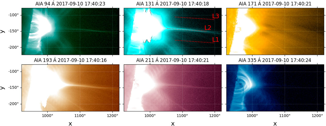
Figure 1. AIA images near 17:40:18 UT of an X8.2 flare occurred on 10 September 2017 (case A). The dotted lines L1–L3 denote the paths for performing SFs.

2.1.2 Case B

Our second plasma sheet example occurred during an X4.9 flare that started at approximately 00:50 UT on 25 February 2014 on the east limb. The plasma sheet lasts over 6 h and has been well observed at 131 Å of SDO/AIA. Unlike a perfect edge-on observing perspective in case A, the observation in case B shows that the plasma sheet is accompanied by a supra-arcade fan and starts to widen at approximately 01:40 UT (Seaton et al., 2017). We select the images at 01:15 UT when the supra-arcade fan has not yet formed and the plasma sheet has not started to widen. The 131 Å observation at this moment captures a long, narrow plasma sheet (the top middle panel in Figure 2). However, pre-existing high-altitude loops and the large complex filament eruption at approximately 00:40 UT (Chen et al., 2014; Seaton et al., 2017) left behind a “plasma cloud” surrounding the plasma sheet, which contaminates the observation of the plasma sheet in the 193 Å channel, where we can only barely recognize the plasma sheet from the surrounding plasma (bottom left panel in Figure 2). As we will show below, case B is a good complement to case A for investigating the possible consequences and cautions of applying SFs to the plasma sheets in wavelength with contamination from other plasma.

Figure 2

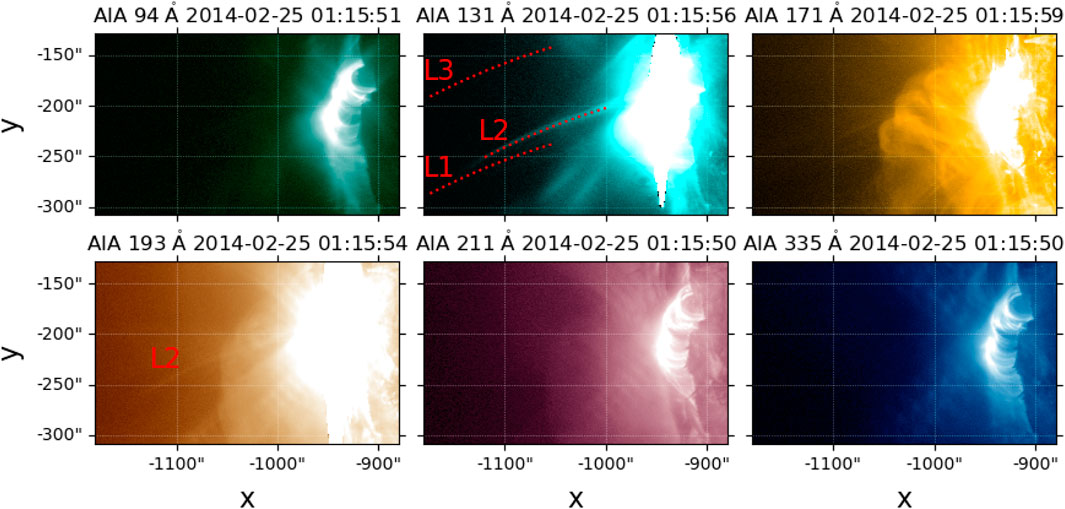
Figure 2. AIA images near 01:15:56 UT of an X4.9 flare occurred on 25 February 2014 (case B). The dotted curves L1–L3 denote the paths for performing SFs. The relative location of “L2” marked on the 193 Å image is the same as on the 131 Å image for helping recognize the plasma sheet from the surrounding plasma on the 193 Å image.

2.2 Structure function

SFs are powerful tools to study homogeneous and stationary turbulence (Frisch, 1995). In our case, we considered a 1D dataset intensity I(x) with N data points in the spatial domain x, and then the kth order SF was computed using

$S_k\left(\tau \right)=<|I\left(x\right)-I\left(x+\tau \right){|}^k>$

where τ is the distance between the spatial points x and x + τ in our case. If the data points are indexed by i = 1, 2, 3, … N, with a uniform data resolution Δ, then S can be computed using

$S_k\left(\tau \right)=<|I_{\left(i\right)}-I_{\left(i+\lfloor \tau /\mathrm{\Delta }\rfloor \right)}{|}^k>$

where i goes from 1 to N − ⌊τ/Δ⌋. We select τ to be a multiple of Δ, so ⌊τ/Δ⌋ = τ/Δ. We require data points to be evenly spaced along the path. This requirement necessitates that, depending on the path we choose, interpolation has to be performed such that the dataset contains data that are location-weighted intensities from the four nearest neighbor pixels. We only consider k = 2 and 3 in this work. For well-developed stationary and homogeneous turbulence, the second-order SF S₂(τ) ∝ τ^γ−1 with the exponent γ related to the spectral index of the corresponding power spectrum in the inertial range (Frisch, 1995). In our study, the EUV observations of current sheets are largely stationary, but due to a radial-dependent density, they are not homogeneous. Consequently, the nominal SF analysis needs to be adapted to our situation. This adaptation is discussed in Section 4.

3 Results for the two selected events

3.1 Case A

Our first step is to test whether the SF is capable of showing significant signatures of turbulence in the plasma sheet, as observed in previous studies (Cheng et al., 2018; Li et al., 2018; Polito et al., 2018; Warren et al., 2018; French et al., 2019; French et al., 2020). We start our tests in the 131 Å channel, which displays the most distinguishable structure of the plasma sheet from the background. The top two rows in the left three columns of Figure 3 show the 131 Å channel intensity as a function of distance along the paths (indicated by dotted lines shown in Figure 1) and the corresponding SF results. We set the leftmost point as our starting point. Path L2 is within the plasma sheet, while paths L1 and L3 are parallel to L2 in the background for comparison. In order to ensure that the spatial interval of points that we select for performing SFs is larger than the spatial resolution of AIA images, we only select 200 points evenly distributed on the paths (the interval of adjacent points corresponds to 1.002 AIA pixels = 0.436 Mm) for this event. The SFs S_k(τ) for k = 2 and 3 are fitted using a power-law function $\sim {\tau }^{{\beta }_k}$ in the range marked by the vertical dashed lines.

Figure 3

Figure 3. (A–C) Intensity versus distance along the paths L1–L3 shown in Figure 1 (case A). We set the leftist location of the path as distance 0. (D–F) Corresponding SF results of the top panels. (G–I) Constructed quasi-homogeneous data from the top panels. (J–L) Corresponding SFs with arbitrary units. A power law fitting for the SF $\sim {\tau }^{{\beta }_k}$ is performed. The fitting range is indicated by two vertical dashed lines. The left three columns are for 131 Å and the right three columns are for 193 Å.

Comparing panels (d), (e), and (f), we see that the index fitted from the SF results within the plasma sheet is significantly greater than the ones in the background. Note that β₂ = 1.36 in panel (e). This value corresponds to a power law index for the power spectrum of δn ∼ δb to be 2.36, much steeper than the Kolmogorov 5/3 (Kolmogorov, 1941) or Iroshnikov–Kraichnan (IK) 3/2 (Iroshnikov, 1964; Kraichnan, 1965) values. In comparison, the value of β₂ = 0.58 in panel (d) and the value of β₂ = 0.62 in panel (f) translate to a power law index for the power spectrum of δn ∼ δb to be $\sim 1.6$, much closer to the Kolmogorov and/or the IK values. One may be tempted to conclude that the observations of background emissions in panels (d) and (f) indicate the presence of MHD turbulence. However, we note that the data along all paths (either within the plasma sheet or on the background) have a radial dependence, i.e., intensity decreases as a function of distance. This situation is similar to that reported in the distribution of electron density from eclipse photometry (Koutchmy, 1994). A radial dependence of intensity has consequences for the SFs.

In order to test the impact of the radial dependence of a dataset on the corresponding SF results, in Section 4.1, we artificially construct data containing no turbulence but with a radial dependence given by I ∼ I₀ (x + d)^α. Figure 8 in Section 4.1 shows five tests where we randomly generate the parameters α (from −2 to 2) and d (from 0.01 to 30). These results demonstrate that a dataset with a radial dependence but no turbulence can lead to SFs showing scaling with the data separation τ, suggesting that the radial dependence property in the data has an impact on SF results.

To remove the impact of radial dependence in the data on the SF results, we multiply the original data by an auxiliary function with an expression of C (x + d)^α to construct quasi-homogeneous datasets. The details of this approach are further discussed in Section 4. After testing, we found that a piecewise functional form,

$C\left(x\right)=C_1{\left(x+d_1\right)}^{{\alpha }_1}*\theta \left(x-x_0\right)+C_2{\left(x+d_2\right)}^{{\alpha }_2}*\theta \left(x-x_0\right),(1)$

where

$C_2=C_1{\left(x_0+d_1\right)}^{{\alpha }_1}*{\left(x_0+d_2\right)}^{-{\alpha }_2}$

and θ(x) is the Heaviside step function, provides a suitable construction of quasi-homogeneous data for both events in this work. The constructed data are displayed in Figures 3G–I in the left three columns, and the corresponding SFs are displayed in Figures 3J–L in the left three columns. The parameters for constructing quasi-homogenous data for the six channels and paths L1–L3 in Figures 3, 5 of case A are provided in Table 1. The choice of constant C₁ is arbitrary and does not have an impact on the indices of SF results. We point out here that the parameters for constructing quasi-homogenous data are not unique, and the discussion on obtaining the parameters for constructing quasi-homogenous data can be found in Section 4.2. The index of the SF from quasi-homogeneous data within the plasma sheet (panel k) is still significantly greater than those in the background (panels j and l), showing that using an SF can effectively detect the presence of turbulence in a dataset containing spatial variation. Now, β₂ = 0.45 in panel (k). This value corresponds to a power law index for the power spectrum of δn ∼ δb to be 1.45, close to the Kraichnan (MHD) 3/2 value. We remark that the profile and index of the SFs in Figure 3 show the property of extended self-similarity (ESS), i.e., 3/2 times the index of the 2nd SF is comparable to the index of the 3rd SF. ESS has been investigated in velocity SFs of turbulence (Benzi et al., 1993; Camussi et al., 1996; Sreenivasan and Antonia, 1997) and has also been shown in the SFs of density in 3D compressible MHD simulations (Kowal et al., 2007) and integrated intensity from observations of interstellar clouds (Padoan et al., 2003). Comparing panels (d), (e), and (f) with panels (j), (k), and (L), it is clear that inhomogeneity can have a significant effect on the resulting SF analysis. It is therefore important to filter out inhomogeneity from the data, as discussed in Section 4.2.

Table 1

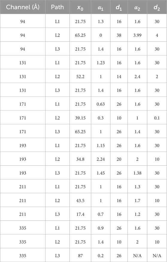
Table 1. Parameters for constructing quasi-homogenous data shown in Figures 3, 5 of case A. The cell displaying N/A corresponds to when x₀ equals the largest x.

As another robust test to confirm the presence of turbulence in our event, we further “shuffle” the data points along the paths in Figure 3 and obtain new data series, as shown in Figure 4. Upon data shuffling, there is no longer evidence of “meaningful” indices of SFs in the shuffled data. The SFs of the shuffled data showed no scale dependence, indicating that the shuffled data are consistent with data series consisting of random variables. Moreover, there is no apparent distinction between indices of SFs of shuffled data within the plasma sheet and the background, confirming that the signals and patterns displayed in Figure 3K in the left three columns are a real property originating from the presence of turbulence rather than instrumental effects (De Moortel et al., 2014). We conclude that shuffling can effectively remove characteristics of the underlying turbulence in the plasma sheet, leading to a background-like data series. The shuffling test gives us confidence that the apparent indices shown in Figure 3K and the difference between the indices within the plasma sheet and the background (Figure 3) confirm the presence of turbulence within the plasma sheet.

Figure 4

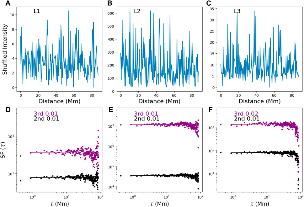
Figure 4. SFs (D–E) on shuffled data (A–C) from original intensity corresponding to panels (A–C) in the left three columns of Figure 3 (case A).

For SFs along the paths L1–L3 at other wavelengths (right three columns of Figure 3; Figure 5), after constructing the homogenous data, only the results at 193 Å show distinguishable signatures of SFs from the background, similar to those at 131 Å, and SF indices in the plasma sheet are slightly larger than those in the background at 94 Å. The temperature response curves for six channels (94 Å, 131 Å, 171 Å, 193 Å, 211 Å, and 335 Å) we analyzed in this study, which can be obtained using the aia_get_response routine in Solar Software (SSW), are shown in Figure 12A. Compared to 131 Å and 193 Å channels, which have their response peaks $>10$ MK, 171 Å, 211 Å, and 335 Å channels are more sensitive to plasma with temperature $<10$ MK (O’Dwyer et al., 2010). Consequently, we expect that the observations in 171 Å, 211 Å, and 335 Å along the plasma sheet are dominated by the background plasma; therefore, in these channels, the plasma sheet and the two background tracks should have SFs with similar behavior. On the other hand, the existence of a temperature response peak slightly below 10 MK enables 94 Å to capture part of the plasma sheet information, leading to slightly larger indices in the plasma sheet of the 94 Å channel than those from the background. However, compared to 131 Å and 193 Å, data from 94 Å is noisier and more contaminated, so we do not use 94 Å to examine the plasma sheet turbulence.

Figure 5

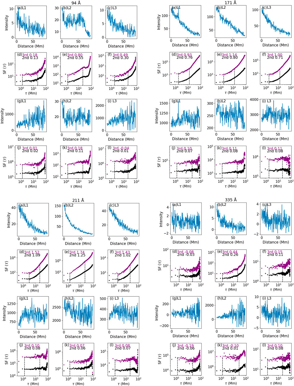
Figure 5. Same as Figure 3, but for 94 Å (top left three columns), 171 Å (top right three columns), 211 Å (bottom left three columns), and 335 Å (bottom right three columns) in case A.

Our tests so far demonstrate that SFs are capable of probing turbulence in the plasma sheet in 131 Å and 193 Å channels that have pronounced temperature response peaks (see Figure 12A) above 10⁷ K. In wavelengths other than 131 Å and 193 Å, there is no apparent distinction between SFs within the plasma sheet and the background.

3.2 Case B

We now discuss case B. Panels (a)–(c) in the left three columns of Figure 6 show the intensity in channel 131 Å for the three paths (one for the plasma sheet and two in the background) shown in Figure 2; panels (d)–(f) of Figure 6 are the SF analysis for the original intensity data; panels (g)–(i) of Figure 6 are the constructed intensity data after removing the radial dependence using Eq. 1. The parameters for constructing quasi-homogenous data for the five channels and paths L1–L3 in Figures 6, 7 of case B are shown in Table 2. The corresponding SF analyses are shown in panels (j)-(L). Similar to case A, the index of SF from quasi-homogeneous data within the plasma sheet (panel k) is significantly greater than those in the background (panels j and l), confirming that using SF can effectively detect the presence of turbulence in case B as well. The fitted value of β₂ = 0.38 in Figure 6K in the left three columns is shallower than β₂ = 0.45 in case A (Figure 3K in the left three columns), indicating event variation. We remark that it will be of great value to perform future statistical analyses of other events to obtain a distribution of the exponent β₂. SFs of the background in case B of 131 Å are flat in shape and noisier than in case A. The right three columns of Figure 6 are for the 193 Å channel in case B. Different from case A, where SFs on 131 Å and 193 Å show close indices, along the plasma sheet path, β₂ in 193 Å of case B is noticeably greater than the β₂ value in 131 Å. Examining the images of case B (Figure 2), we can see that there is a plasma cloud around the plasma sheet in 193 Å in the aftermath of a complex filament eruption. Therefore, the observed intensity along L2 in 193 Å of case B is the combination of the plasma sheet and plasma cloud. The relatively cooler plasma cloud is more pronounced at 193 Å than at 131 Å, and it is the most visible in the 171 Å channel. We see that the “contamination” from the plasma cloud can have a considerable impact on SFs. It is therefore necessary to be cautious about the contamination effects when performing SFs on emissions. The more distinctive a structure, such as a plasma sheet, is from the background, the more applicable it is to perform SF analysis on this structure.

Figure 6

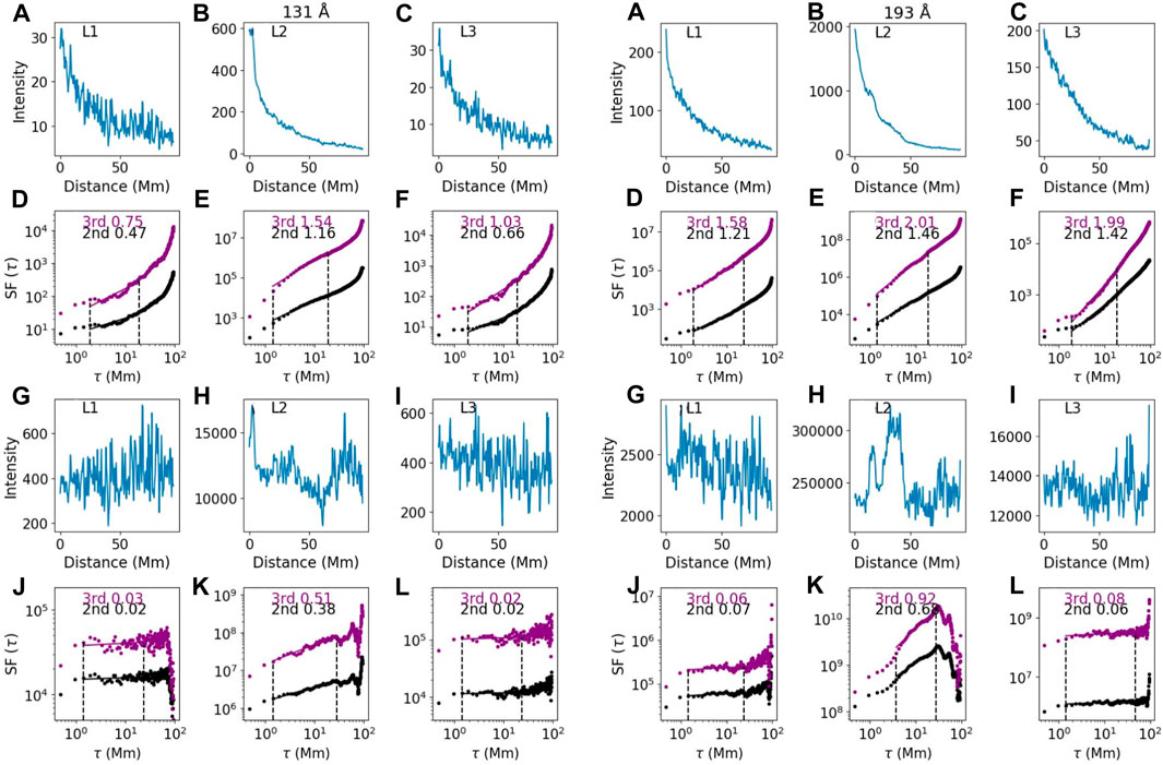
Figure 6. (A–C) Intensity versusdistance along the paths L1–L3 shown in Figure 2 (case B); (D–F) corresponding SF results of the top panels; (G–I) constructed quasi-homogenous data from the top panels, and (J–L)corresponding SFs with arbitrary units. The fitting range is indicated by two vertical dashed lines. The left three columns are for 131 Å and the right three columns are for 193 Å.

Table 2

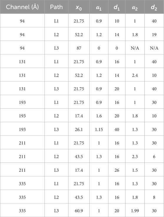
Table 2. Parameters for constructing quasi-homogenous data shown in Figures 6, 7 of case B. The cell displaying N/A corresponds to when x₀equals the largest x.

The SFs on other wavelengths in case B (Figure 7) show similar results as in case A; i.e., there is no noticeable distinction between the SFs in the plasma sheet and the background in 211 Å and 335 Å. The 94 Å emission shows slightly larger indices of the SF in the plasma sheet than in the background, but the difference is not large enough to trustfully claim the existence of turbulence within the plasma sheet. We do not perform SFs along L2 in 171 Å for case B since the emission in 171 Å is dominated by the plasma cloud instead of the plasma sheet (see Figure 2). The intention of this paper is to test the ability of adopted SFs to probe turbulence, and the properties of turbulence in different structures are beyond the scope of the current research. In a future paper, we will study turbulence in loop structures using the procedures developed here.

Figure 7

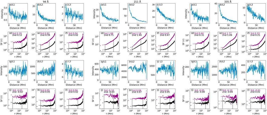
Figure 7. Same as Figure 6 but for 94 Å (left three columns), 211 Å (middle three columns), and 335 Å (right three columns) in case B.

4 Structure function analysis and its validation

In this section, we validate our procedures by performing various tests on synthetic data. In Section 4.1, we examine SFs for the dataset with the prescribed radial dependence without turbulence. Data with a radial dependence is non-homogeneous. When applying SF analyses, we find the corresponding SFs will exhibit power law behavior, which could be wrongly interpreted as signatures of turbulence. In Section 4.2, we examine how one can remove (large scale) radial dependence of a dataset with synthetic turbulence. We show that different functional forms for removing the radial dependence in the dataset can be used, and they yield similar SF. These tests, therefore, provide a validation test for our procedure.

4.1 Effect of turbulence-free but spatial-dependent data on SFs

Consider intensity data with a radial dependence given by

$I\left(x\right)=I_0*{\left(x+d\right)}^{\alpha }$

In Figure 8, we randomly generate the parameters α (from −2 to 0) and d (from 0.1 to 30) and construct I(x) (shown in panels (a)–(e)) to test the impact of the radial dependence of a dataset on the corresponding SFs (shown in panels (f)–(j)). Figure 8 illustrates that a dataset with a radial dependence but no turbulence can lead to a non-zero index for the resulting SFs. The intensities shown in panels a–c in Figures 3, 5, 7 have clear radial dependence. Therefore, it is necessary to remove any radial dependence from the data before SF analysis. In Section 4.2, we describe and validate our approach of constructing quasi-homogenous data and show that its robustness by testing it on synthetic turbulence.

Figure 8

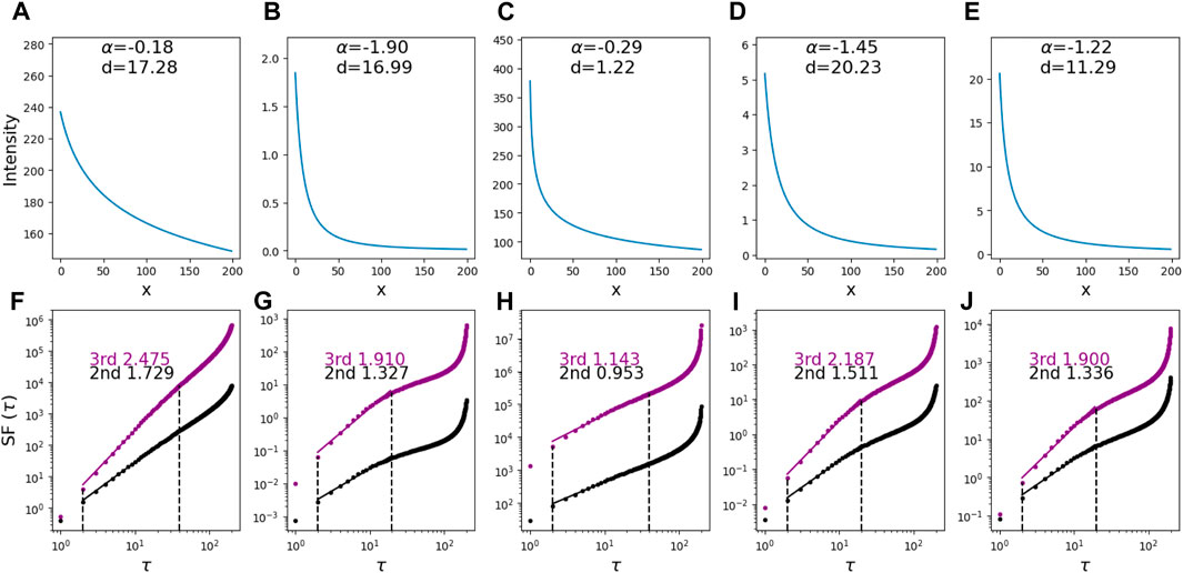
Figure 8. SFs (F–J) on test data (A–E) with radial dependent I₀ (x + d)^α and contains no turbulence.

4.2 SFs of synthetic turbulence with radial dependence

A key step in our analysis is the reconstruction of a new dataset from the original data by removing a large-scale radial dependence of the original data. This step is necessary because a large-scale radial dependence in the data can affect the SF analysis. Since the exact radial dependence is not known, the procedures for removing the large-scale radial dependence are not unique, so it is also important to examine whether the SF analysis sensitively depends on the choice of this removal procedure. We use synthetic turbulence to test the applicability and robustness of our procedures.

For our problem of a plasma sheet, the geometry is 1D. So, we construct a 1D model of intensity from synthetic 1D turbulence. We then apply our procedures to compute the corresponding SFs and obtain their scaling power-law indices. These indices are compared with the spectral indices of the input turbulence. For testing purposes, we consider number density n for our analysis. The turbulence is added as sinusoidal waves with wave number k_i. The smallest k_i is decided by the length scale L of the problem. The total number density n is now

$n=n_0+\delta n,n_0=\mathrm{c}\mathrm{o}\mathrm{n}\mathrm{s}\mathrm{t}\mathrm{a}\mathrm{n}\mathrm{t},\delta n={\displaystyle \sum _{i=1}^N}A\left(k_i\right)\text{exp}\left(i\left(k_{i}x+{\gamma }_i\right)\right)$

$P\left(k_i\right)=\frac{1}{{\left(1+{\left(k_i\lambda \right)}^2\right)}^{5/6}},A^2\left(k_i\right)=\frac{{\sigma }_{n}P\left(k_i\right)}{{\sum }_1^{N}P\left(k_i\right)},{\sigma }_n=<{\left(\delta n\right)}^2>,(2)$

where P(k) is the power associated with δn and is chosen to be Kolmogorov-like at large k. We choose L = 70 Mm, λ = 0.03L, and N = 1000. We have $k_1=\frac{2\pi }{L}$ and k_j = jk₁ for j = 2 to N.

Figure 9A shows the synthetic turbulent density with n₀ = 40 and σ_n = 1. This choice of σ_n gives δ_n/n₀ ∼ 2.5%, satisfying δ_n ≪ n₀. The corresponding SFs are shown in Figure 9G. Between the two dashed lines, the second-order SF scales as τ^0.62, which translates to a power spectrum ∼ k^−1.62, shallower but close to the input ∼ k^−1.67. Since the EUV intensity is proportional to n², in panel (b), we examine the distribution of ${(n_0+\delta n)}^2$. The corresponding SFs, shown in Figure 9H, are similar to those shown in Figure 9G. This result is expected because ${(n_0+\delta n)}^2=n_0^2+2n_0\delta n+{(\delta n)}^2$. When δn ≪ n₀, the SFs of n² behave like 2n₀δn. Next, we include a x (radius) dependence to the synthetic intensity as

$I_{\mathit{syn}}=62.5{\left(n_0+\delta n\right)}^2{\left(x+30\right)}^{-1.2}.(3)$

Figure 9

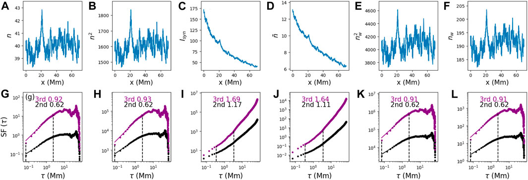
Figure 9. (A) Number density n of synthetic turbulence, with n₀ = 40 and σ_n = 1; (B) n²; (C) n² with the modulation of radial dependence; (D) square root of the data in (C); (E) constructed quasi-homogenous data from (C); and (F) constructed quasi-homogenous data from (D). Bottom panels (G–L) represent the corresponding SF results of the data in the top panels (A–F).

We point out here that, for synthetic intensity, the choices of the constants for radial dependence are not unique. The selection of constants “62.5, 30, and −1.2” in Eq. 3 is because this selection leads to a similar intensity profile between Figure 9C and Figure 3B of the left three columns, which would make it easier for us to understand the examination procedures on synthetic turbulence in the observational context of the current paper. The intensity synthesized using Eq. 3 is shown in Figure 9C. Figure 9D is the inferred density $\tilde{n}\sim \sqrt{I_{\mathit{syn}}}$. The corresponding SFs for I_syn and $\tilde{n}$ are shown in panels (i) and (j), respectively. Comparing panel (i) with panel (g) and panel (j) with panel (h), we see that the radial dependence of I_syn and $\tilde{n}$ affects their SFs, leading to a stronger scaling of τ^1.17 and τ^1.11. If one were to interpret these scalings as signatures of turbulence, one would obtain erroneous power spectra of ∼ k^−2.17 and ∼ k^−2.11, which are softer than the input spectrum ∼ k^−1.67.

Note that the SF analyses in panels (i) and (j) of Figure 9 depend on the level of σ_n. In Figure 10, where σ_n = 4 and we apply the same radial dependence as in Figure 9, we see that the corresponding SFs, shown in panels (i) and (j) in Figure 10, are “harder” than those in Figure 9. On the contrary, panels (k) and (l) in Figure 9 and Figure 10 are similar. This observation implies that if one were to directly apply the SF analysis to some radial-dependent intensity data, then the results would be event-dependent, and the resulting turbulence power spectral index may have a large range.

Figure 10

Figure 10. Same as Figure 9 but with σ_n = 4.

We now test whether we can use the procedures by which we process the observation data on this intentionally constructed radially dependent data to obtain the correct power spectrum index. In analogy to observations, we treat the data in Figure 9D, which is $\tilde{n}(x)$, as an unknown trend and use a piecewise function f(x) to obtain a new dataset, denoted as n_w(x) through $n_w(x)=\tilde{n}(x)*f(x)$. The piecewise function is chosen so that n_w(x) is quasi-homogenous (the exact form of f(x) is not important, as we discuss below). For our problem, we chose f₁(x) to be

$f_1\left(x\right)=\left\{\begin{array}{cc}{\left(x+40\right)}^{0.73}\hfill & x\le 21\mathrm{M}\mathrm{m}\hfill \\ C{\left(x+18\right)}^{0.5}\hfill & x>21\mathrm{M}\mathrm{m}\hfill \end{array}\right.,$

where C = (21 + 18)^−0.5*(21 + 40)^0.73 is a constant. The new dataset n_w(x) is shown in Figure 9F. Figure 9F is statistically similar to Figure 9A, as the dots of n as a function of n_w distribute closely along a linear line (not shown in the paper), although the magnitude is different. This difference is not a concern since the power law index from the SF analysis does not depend on the magnitude of the data. The SF analysis of Figure 9F is shown in Figure 9L. We see that the SF results in Figure 9F are the same as those shown in Figure 9G, which is for the original data. Note that our “trial” piecewise function is not the inverse of the square root of Eq. 3, yet the SFs for the constructed density (Figure 9L) and the original synthetic turbulence density (Figure 9G) are very similar. We have tried other piecewise functions, such as

$f_2\left(x\right)=\left\{\begin{array}{cc}{\left(x+50\right)}^{0.87}\hfill & x\le 38.5\mathrm{M}\mathrm{m}\hfill \\ C{\left(x+9\right)}^{0.43}\hfill & x>38.5\mathrm{M}\mathrm{m}\hfill \end{array}\right.,$

where C = (38.5 + 9)^−0.43*(38.5 + 50)^0.87, and found that as long as no clear radial trend is seen after we apply the piecewise function, the corresponding SFs show similar power law indices as those in panel (g). This result demonstrates the effectiveness and robustness of our procedures in revealing the true properties of the turbulence.

The choices of the parameters to construct quasi-homogeneous data to reveal turbulence characteristics in the original data are not unique. One can try different empirical parameters to construct quasi-homogeneous data. There are no clear criteria to evaluate these choices, and statistically, we expect them to be similar. Visual inspection is helpful in constructing the quasi-homogeneity of the data, and the statistical similarity and similar indices of the corresponding SFs between the “trial” groups are an indicator that the parameters chosen for constructing the data are good enough to retrieve the turbulence information in the system. Indeed, in our practices, we find that choosing different empirical formulas yields similar SFs. This suggests that the resulting SFs are robust, and removing the radial dependence is important. Since radial dependence exists in most cases of solar EUV and white light observations, the lack of constructing quasi-homogeneous data and directly applying SF to original observational data would lead to erroneous conclusions.

The above point is illustrated in the concrete example shown in Figure 9. The original homogeneous turbulence is shown in panel (a). The constructed non-homogeneous turbulence is shown in panel (d). To examine the turbulence characteristics from panel (d), however, one does not need to strictly apply C (x + 30)^0.6, as shown in Figure 9D. Instead, applying different forms of piecewise functions f₁(x), or f₂(x), or other forms (that we tried but are not shown here) to the synthetic intensity can equally well reconstruct quasi-homogeneous data from which the characteristics of original turbulence can be obtained. These are shown in Figures 9F, L. These results show that we do not need to impose strict requirements on the reconstruction procedures to obtain quasi-homogeneous data. In practice, multiple reconstruction procedures should be tested and examined, and their results should be compared. If these results are similar, they testify to the robustness of these reconstruction procedures (as in our two examples). The fact that multiple choices of reconstruction lead to similar results (e.g., SFs) is important for observational data analysis since we do not know the exact radial dependence from the observations themselves. We remark that the exact form of the reconstruction is not important, but removing the radial dependence from the data to obtain quasi-homogeneous data, as proposed in the current paper, is important.

If the selections of the parameters for constructing the quasi-homogeneous data are not unique, there may be concerns that the similar results are due to the construction process itself, which could add some systematic biases to, e.g., the spectral indices of turbulence. To check on that, we further examine the synthetic turbulence with P (k_i) chosen to be Iroshnikov–Kraichnan (IK)-like at large k (i.e., changing index from “5/6” to “3/4” in P (k_i) of Eq. 2). The results are shown in Figure 11. Different P (k_i) distributions for synthetic turbulence reflected in different SF indices between Figure 9G and Figure 11G. After we use the same radial dependence as in Figure 9 (Eq. 3) to obtain synthetic intensity in Figure 11C and inferred density $\tilde{n}\sim \sqrt{I_{\mathit{syn}}}$ in Figure 11D, we apply f₁(x) to construct quasi-homogeneous data, as shown in Figure 11F. Comparing Figures 11A,F and their corresponding SF results (Figure 11L, G), we note that applying f₁(x) successfully retrieves the information regarding the synthetic turbulence, and we obtain the same SF results in Figure 11L as in the original turbulence in Figure 11G. More importantly, we see that applying the same auxiliary function f₁(x) to construct quasi-homogeneous data does not give the same index of SFs between Figure 9L and Figure 11L but retrieves back the SF index of the original synthetic turbulence. We further apply other auxiliary functions, including f₂(x) to Figure 11D, and the results are similar to those shown in Figures 11F, L (not shown in the paper).

Figure 11

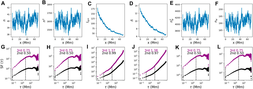
Figure 11. Same as Figure 9 but with P(k) chosen to be Iroshnikov–Kraichnan (IK)-like at large k (i.e., changing index from “5/6” to “3/4” in P(k_i) of Eq. 2).

Applying the piecewise function to the radially dependent intensity data in Figure 9C, we obtain the constructed intensity, denoted as $n_w^2$, as shown in Figure 9E. The corresponding SFs are shown in Figure 9K. Again, we see that Figure 9K is very similar to Figures 9G, H. Finally, the fact that Figures 9K, L are very similar ensures that we can directly examine intensity data from the observation without first obtaining the density from the intensity. In Section 4.3, we discuss how one can obtain density data from intensities from multiple channels and the corresponding SF analysis on the density data. We remark that our approach of using intensity data to probe the underlying turbulence property is straightforward and easy to implement. Therefore, it can be conveniently applied to massive SDO/AIA data.

4.3 SF analysis of the number density

If we obtain the plasma density from measurements of intensities at multiple wavelengths, then it is possible to examine the turbulent plasma density directly. There are two mainstream approaches to obtaining plasma density from intensity observations. The first one makes use of the ratio of intensities in two channels, and the second is the so-called differential emission measure (DEM) analysis, which uses as many channels as possible. These approaches differ in their assumptions about the plasma temperature and are used in different situations. Here, we show readers examples using both approaches. The results differ, and we explain the reasons behind this variation.

The first approach derives the number density using the ratio of intensities only from two channels. This has been practiced by Petkaki et al. (2012); Del Zanna and Woods (2013); Polito et al. (2017); Mulay et al. (2021). Using this approach, plasma is assumed to be isothermal with temperature T₀ and uniformly distributed along the line of sight (LOS), and the intensity in channel i can then be expressed as

$I_i=R_i\left(T_0\right)n^2\left(T_0\right)l,(4)$

where R_i (T₀) is the SDO/AIA temperature response function for i bandpass (shown in Figure 12A) at temperature T₀ and l is the length of LOS of the plasma sheet. The ratio of the intensities of channels i to j can then be written as

$\frac{I_i}{I_j}=\frac{R_i\left(T_0\right)n^2\left(T_0\right)l}{R_j\left(T_0\right)n^2\left(T_0\right)l}=\frac{R_i\left(T_0\right)}{R_j\left(T_0\right)}.(5)$

Figure 12

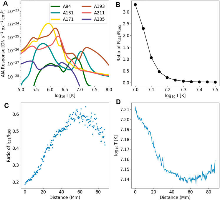
Figure 12. (A) SDO/AIA temperature response of six wavelengths dominated by emissions from iron lines on 10 September 2017 (case A); (B) ratio of the response function of 131 Å to 193 Å in the range of 10⁷–10^7.5 K; (C) ratio of intensity in 131 Å (I₁₃₁) to intensity in 193 Å (I₁₉₃) as a function of distance along path L2 in case A; and (D) derived temperature as a function of distance along L2.

Previous studies (Cheng et al., 2018; Warren et al., 2018; French et al., 2020) demonstrated that the temperature within the plasma sheet in case A studied here is in a narrow range of 10⁷–10^7.5K. As the ratio of response functions of 131 Å to 193 Å (R₁₃₁/R₁₉₃) monotonically decreases as a function of temperature within this range (Figure 12B), we can obtain the corresponding T₀ from the curve of R₁₃₁/R₁₉₃ using the ratio of intensities of 131 Å to 193 Å (I₁₃₁/I₁₉₃) from the observations. The number density can therefore be obtained by substituting T₀ in Eq. 4.

The two wavelengths that are most sensitive in the high-temperature range ($\ge 10^7$ K) in SDO/AIA are 131 Å and 193 Å. They are used to derive T₀ according to Eq. 5. As the plasma sheet structure from 131 Å and 193 Å images is at least 10 times greater than the background (see Figure 3), we can treat the derived density along L2 from the ratio of 131 Å to 193 Å as the density of the hot plasma sheet. This procedure can be conducted for any single pixel to obtain its density and temperature.

In Figures 12C, D, we show I₁₃₁/I₁₉₃ and temperature as a function of distance along the plasma sheet. With the same assumption of the depth of LOS as in Cheng et al. (2018), we derive n (T₀) as a function of distance from 131 Å using Eq. 4. This density is shown in Figure 13A. The derived density is consistent with the order of magnitude of density derived by Cheng et al. (2018), Warren et al. (2018), and French et al. (2019). We then construct quasi-homogenous data from n (T₀) (denoted as n hereafter), which is shown in Figure 13B.

Figure 13

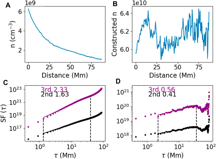
Figure 13. (A) Density as a function of distance along L2 in case A derived from the approach of the ratio of intensities; (B) quasi-homogenous density constructed from (A); and (C,D) corresponding SFs of the top panels.

Figures 13C,D are SFs corresponding to panels (a) and (b), respectively. These SFs are slightly different from but consistent with those of the intensity SFs in Figure 3. Note that, intensities from two channels are needed to obtain the density using this approach. Furthermore, emissions from the two channels must predominantly come from the plasma sheet.

For case B of our study, however, we have only one channel (131 Å) that has emissions dominantly from the plasma sheet, implying that we cannot use the ratio of intensities to deduce density in case B. Nevertheless, based on the discussion above and the fact that the plasma sheet is distinctively observed at 131 Å, we expect the characteristics of SFs at 131 Å after construction to reveal the turbulence property in density according to Eq. 4.

The second method to derive plasma density is DEM analysis. It also yields plasma temperature information. The methodology for using DEMs to derive plasma density and temperature can be found in Section 3.1 of Xie and Revees (2023) and the references therein. In particular, we use the approach of regularized inversion developed by Hannah and Kontar (2012) and Hannah and Kontar (2013). After obtaining DEMs, we can calculate the total emission measure (EM) using

$EM\left(T\right)=\int \mathrm{D}\mathrm{E}\mathrm{M}\left(T\right)dT$

and we can derive the number density of electrons using

$n=\sqrt{\mathrm{E}\mathrm{M}/l}$

where l is the depth of LOS under the assumption that the plasma is uniform along the LOS (Reeves et al., 2017; Xue et al., 2020; Xie and Reeves, 2023).

In practice, we use 41 temperature bins (10^5.7 K–10^7.6 K) with the interval Δlog T evenly distributed. We write intensity in the ith channel, F_i, in the following form:

$\begin{array}{ll}\hfill F_i& ={\displaystyle \sum _{n=0}^{40}}{R}_i\left(T_n\right)\times \mathrm{D}\mathrm{E}\mathrm{M}\left(T_n\right)\mathrm{\Delta }{T}_n\hfill \\ \hfill & ={\displaystyle \sum _{n=0}^{40}}{R}_i\left(T_n\right)\times EM\left(T_n\right).\hfill \end{array}(6)$

Eq. 6 demonstrates that F_i is the linear combination of EM(T_n) in various temperature bins with the weight of R_i (T_n). Eq. 6 becomes Eq. 4 if we assume that plasma is isothermal, i.e., there is only one temperature bin in Eq. 6.

Figure 14 shows the DEM distribution along the plasma sheet for case A. It shows that there are likely to be two populations of plasma. The dominant one has a temperature between 10⁷ K and 10^7.5 K, and the minor one has a temperature of $\sim 10^{6.5}$ K. The lower temperature population is likely from the foreground and background, and the higher temperature population is the hot plasma in the plasma sheet. This figure justifies our assumption that the temperature of the plasma sheet in case A is in the range of 10⁷–10^7.5 K when using the ratio of intensities to obtain the density. The DEM-weighted mean temperature (right panel in Figure 14) and temperature derived from the ratio of intensities (Figure 12D) show a similar trend, i.e., the temperature decreases as a function of distance within 0–50 Mm.

Figure 14

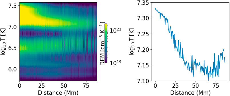
Figure 14. DEM distribution along the path L2 (lsft panle) and DEM-weighted temperature as a function of distance (right panel) in case (A).

Figure 15 shows the SF results on EMs in dominant temperature bins. From left to right, the range of these temperatures is log₁₀T (K): 7.14–7.18, 7.18–7.23, 7.23–7.28, and 7.28–7.32, respectively. In computing the SFs, we only include points with non-zero emission measures. Compared to SFs from the intensities at 131 Å and 193 Å, the SFs for EMs in these four dominant temperature bins show rather shallow τ scaling. The scaling exponents for the second SFs are 0.16, 0.21, 0.13, and 0.29. If δn is randomly distributed (e.g., upon performing data shuffling), we expect the SFs to have no τ dependence and the scaling exponents to be consistently zero. The fact that the scaling exponents are now non-zero suggests that there is some “residual” turbulence contained in the EM data.

Figure 15

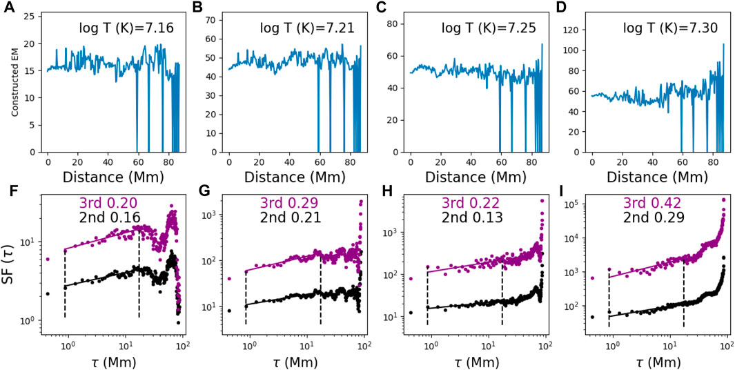
Figure 15. (A–D): constructed quasi-homogenous data from EMs along path L2 in several dominant temperature bins of DEMs in case A. (F–I): corresponding SFs of the top panels.

One reason that the SFs in Figure 15 do not show strong signatures of turbulence could be that in obtaining the EMs using the DEM approach, uncertainties related to the procedures were introduced to the EMs, and these uncertainties contaminate the SF analysis. To test this hypothesis, we compute the EUV intensity from the DEM results using Formula 6 and compare it with the observed intensity at all six wavelengths of AIA/SDO. The results are shown in Figure 16. In each panel, the x-axis is the observed intensity, and the y-axis is the reconstructed intensity from the DEM results. We see that for the 193 Å channel, the intensities reconstructed from the DEM results agree nicely with the observation. For the 211 Å channel, the agreements are reasonable, although we see that the reconstructed intensities near the starting point are systematically smaller than those from the observation. For all other channels, the reconstructed intensities show clear differences from the observations. These disagreements suggest that the procedure of obtaining EM from individual intensity channels may introduce uncertainties, which, as we argued above, may contaminate the SF analysis.

Figure 16

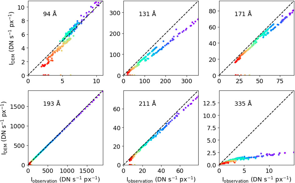
Figure 16. Synthetic intensity versus observed intensity in wavelengths used for deriving DEMs in case A. Colors of data points indicate the distance from the starting point of L2. Points in violet (red) are closer to (further away from) the starting point. The dashed line with slope 1 corresponds to the case where the reconstructed and observed intensities agree.

Comparing the above two approaches, it seems that for our problem, the approach of using intensity ratio provides a better estimate of the plasma density than the DEM method, as long as hot temperatures can be assumed. We attribute this to the fact that the plasma in the plasma sheet is in a narrow temperature bin. In a situation where the plasma contains multiple temperature components, the DEM method will be more applicable than the intensity ratio approach since the latter assumes that the plasma in consideration is in an isothermal state.

Although employing the ratio of intensities is more suitable for our case to derive density, it requires at least two channels that have emissions dominantly from the plasma sheet, and the ratio of the two channels monotonically changes as a function of temperature in the range associated with the structure, which may be a requirement that is hard to meet. This strict requirement is further validated in case B, where the plasma cloud can only be distinctively recognized at 171 Å. However, to probe the turbulence property, we do not need to apply the SF analysis to density. As examined in this work, we can directly examine the intensity of EUV in the channel, which has emissions dominated by the structure that we are interested in studying. A cartoon showing the steps of using EUV intensity observations to probe turbulence in the current sheet is shown in Figure 17. Given the massive SDO/AIA data, our approach will be a powerful tool to examine plasma turbulence in the solar atmosphere.

Figure 17

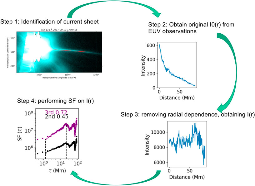
Figure 17. Cartoon that shows the procedure of using EUV intensity to probe turbulence in the current sheet as discussed in this work.

5 Discussion and conclusion

Turbulence is ubiquitous in the solar atmosphere and solar wind. Our understanding of turbulence in the solar wind is inspired by in situ observations. Early investigations from the Helios mission (Bavassano et al., 1982a; Bavassano et al., 1982b) confirmed that the solar wind turbulence evolves radially. A natural question to ask is therefore, what is the turbulence property closer to the Sun in the solar atmosphere? With the launch of the Parker Solar Probe mission, one can now study solar wind turbulence within the young solar wind streams in the vicinity of the Sun, as close as 10R_s (McManus et al., 2020; Fargette et al., 2021; Fargette et al., 2022). Furthermore, however, no in situ observations are available, and one has to rely on remote sensing observations to study turbulence in the solar atmosphere.

Studying turbulence via remote-sensing observations has been practiced before. For example, from radio emissions, scientists have inferred the properties of turbulence in the interstellar medium (Mutel et al., 1974; Lee and Jokipii, 1976; Rickett, 1977; Armstrong et al., 1981; Armstrong et al., 1995) and solar corona (Kontar et al., 2017b; Chen X. et al., 2020; Sharma and Oberoi, 2020; Mohan, 2021). In the study of interstellar scintillation, Armstrong et al. (1981) established a composite power spectrum of electron density that behaves like a power law and is consistent with Kolmogorov turbulence across 12 orders of magnitude of scales. These authors assumed that density fluctuations are proportional to velocity fluctuations, which was also applied in the studies of turbulence in the solar wind, e.g., in Neugebauer et al. (1978).

Density fluctuations can also lead to intensity fluctuations in observations. Using the SF method, Padoan et al. (2023) examined the ¹³CO intensity of molecular clouds to reveal the characteristics of supersonic turbulence in these clouds. They assumed that the integrated intensity could be obtained from column densities by multiplication of a factor (Ossenkopf, 2002). The proportional relationship between density and velocity is the basic assumption in our current work as well. Furthermore, realizing the relationship between $\delta n\sim {(n_0+\delta n)}^2\sim \delta I$ inspired us to test the SF on intensity.

In studying solar plasma, Cheng et al. (2018) used the power spectrum of intensity from EUV emissions to argue the existence of turbulence in the plasma sheet. This work was followed by Liu and Wang (2021), who examined turbulence properties in supra-arcade fans. However, upon reproducing their analyses, we found that the traditional power spectrum method, based on the direct Fourier transform of the intensity profiles, does not clearly distinguish the signatures of turbulence within the plasma sheet and the background. In contrast, we found that the SF of intensity displays significant differences between the plasma sheet and the background.

In this work, we use the intensities of EUV lines from AIA measurements to infer the presence of turbulence in flare plasma sheets. We use SFs, specifically the second-order spatial SF, to detect the presence of turbulence in plasma sheets. We start our test on a well-studied plasma sheet that occurred on 10 September 2017 (case A), in which the existence of turbulence has been inferred from previous studies through spectroscopic observations (Li et al., 2018; Warren et al., 2018; French et al., 2019; French et al., 2020). The results demonstrated that our adopted SF is capable of effectively detecting the presence of turbulence within the plasma sheet. The index of the SF spectrum within the plasma sheet (case A) corresponds to a value close to the Kraichnan (MHD) turbulence. The profile and index of the SFs within the plasma sheet show the property of ESS, which has been investigated in velocity SFs of turbulence (Benzi et al., 1993; Camussi et al., 1996; Sreenivasan and Antonia, 1997), the SFs of density in 3D compressible MHD simulations (Kowal et al., 2007), and integrated intensity from observations of interstellar clouds (Padoan et al., 2003). The index of the SF spectrum within the plasma sheet of our case B is shallower than that in case A, indicating that there is variation in the turbulence properties from event to event. In the current study, we set a strict requirement of at least 200 data samples and the distance between adjacent data points to be larger than the spatial resolution of AIA images. This requirement significantly limits the candidates available for our study based on the many observations of plasma sheets in SDO/AIA. The criteria may be relaxed in future studies, and it will be of great value to perform future statistical analysis of more events to obtain a distribution of the index of the SF spectrum.

When using the SF method (and the traditional power spectral analysis), it is important to first construct quasi-homogenous datasets by removing the radial dependence of the data. A dataset containing a large-scale radial dependence can impact the SF analysis, leading to erroneous conclusions on the properties of the turbulence of the plasma examined. More fundamentally, because the EUV intensity of a plasma sheet decreases radially, the turbulence in plasma sheets is inhomogeneous. This situation is very different from that in the solar wind and the interstellar medium (Mutel et al., 1974; Lee and Jokipii, 1976; Armstrong et al., 1981). Furthermore, for our analyses, we find that only channels that show strong emissions from the structures can yield information about the turbulence in the structure. For plasma sheets in solar flares, high-temperature channels at 131 Å and 193 Å are the primary target channels.

The ability to use SFs to probe turbulence from intensity after removing the radial dependence stems from the relationship $\delta n\sim {(n_0+\delta n)}^2\sim \delta I$. This relationship is verified by our tests on synthetic turbulence in Section 4.2. Restoring the turbulence information in synthetic data using the same procedures as in the observations shows the capability of our approach to restore the information about turbulence. Moreover, the results that are statistically similar to turbulence distribution and the same indices of SF spectra can be obtained by intentionally applying different auxiliary functions to illustrate the robustness of our approach. The fact that there is no apparent distinction between indices of SFs of shuffled data within the plasma sheet and the background after shuffling confirms that the signals and patterns displayed in our analyses of the plasma sheet are real properties originating from the presence of turbulence rather than instrumental effects.

In Section 4.3, we further show that the index of SFs on the density of the plasma sheet is close to the index of SFs on emissions in the channels corresponding to high temperatures, which confirms our adoption of SFs as a useful tool to probe turbulence. Compared to in situ observations, which are mostly one-point in nature, performing SFs on EUV emissions observed from SDO/AIA allows the direct examination of turbulence in the wave-vector space. With massive SDO/AIA observations available, the procedures we developed here can serve as a handy tool to investigate turbulence in the solar atmosphere.

The presence of turbulence in solar flares can be inferred from temporal evolution of EUV images of, e.g., loop structures. During solar flares, there are often significant dynamic changes at the flare site, which is associated with the magnetic reconnection process. Magnetic reconnection drives turbulence and structures are results of these turbulent reconnections. We remark that the environment in the plasma sheet chosen in our study differs significantly from those in the loops. The time of the plasma sheet we chose was before the plasma sheet became widened; therefore, the system was stationary. The loop system, however, was dynamic and non-stationary. We also remark that the emergence of structures is a general property of turbulence. In solar wind MHD turbulence, small-scale structures can emerge, which manifest intermittency for a stationary and uniform system. Current sheets are one of the most popular structures in the solar wind. Li (2008) developed a method to identify these structures and using this method. Li et al. (2011) showed that these structures can affect the power spectrum analysis.

We note that there are other remote sensing measurements that can be useful to study turbulence in the solar atmosphere in the literature. For example, measurements from the Coronal Multi-channel Polarimeter (CoMP and its upgraded version UCoMP) and Daniel K. Inouye Solar Telescope (DKIST) can provide line-of-sight velocity profiles for regions of interest. Recently, using the observations of Doppler shift from CoMP and UCoMP, Sharma and Morton (2023) measured the perpendicular correlation length of Alfvénic waves, therefore providing a constraint for modeling Alfvénic wave turbulence. De Moortel et al. (2014) showed the propagation of transverse perturbations (Doppler shift observed by CoMP) propagating from footpoints to the apex of the loop. The power spectra of Doppler shifts within the loop display higher power in high frequency at the apex than at the footpoints, suggesting possible evidence for Alfvénic turbulence within the loop as the interaction between intensity perturbations and transverse perturbations is a possible scenario leading to Alfvénic turbulence (McIntosh et al., 2013). Combining the current study with other remote sensing observations of velocities, e.g., the observations from CoMP and UCoMP, Doppler and non-thermal velocities from spectroscopic diagnosis from the interface region imaging spectrograph (IRIS), and the extreme ultraviolet imaging spectrometer (EIS) onboard Hinode, should be performed in the future. Finally, we will extend the current procedure to time sequence data at different spatial locations. Such a practice will allow us to examine the temporal behavior of the turbulence in the solar atmosphere.

Data availability statement

The original contributions presented in the study are included in the article/Supplementary Material; further inquiries can be directed to the corresponding author.

Author contributions

XX: writing–original draft and writing–review and editing. GL: writing–original draft and writing–review and editing. KR: writing–review and editing. TG: writing–review and editing.

Funding

The author(s) declare that financial support was received for the research, authorship, and/or publication of this article. XX and KR are supported by NASA (grant 80NSSC18K0732). KR also acknowledges support from NASA (grant 80NSSC19K0853). GL acknowledges support from ISSI and ISSI-BJ through the international team 581. TG acknowledges support from contract SP02H1701R from Lockheed–Martin to SAO.

Acknowledgments

The authors are grateful for the discussions with Dr. Chengcai Shen and Soumya Roy on the thermodynamic properties of plasma sheets and DEMs. The authors thank Drs. Michael Terres, Joel Allred, Graham Kerr, Rohit Chhiber, and William Setterberg for the comments and suggestions on turbulence. Comments and suggestions from the reviewers have helped in improving this paper. For that the authors thank the referees. The AIA data are provided courtesy of NASA/SDO and the AIA science team. The Solar Software (SSW) system is built from Yohkoh, SOHO, SDAC, and Astronomy libraries and draws upon contributions from many members of those projects. CHIANTI is a collaborative project involving George Mason University, the University of Michigan (United States), and the University of Cambridge (United Kingdom).

Conflict of interest

Author GL was employed by General Linear Space Plasma Lab LLC.

The remaining authors declare that the research was conducted in the absence of any commercial or financial relationships that could be construed as a potential conflict of interest.

Publisher’s note

All claims expressed in this article are solely those of the authors and do not necessarily represent those of their affiliated organizations, or those of the publisher, the editors, and the reviewers. Any product that may be evaluated in this article, or claim that may be made by its manufacturer, is not guaranteed or endorsed by the publisher.

References

Allred, J. C., Kerr, G. S., and Gordon Emslie, A. (2022). Solar flare heating with turbulent suppression of thermal conduction. ApJ 931, 60. doi:10.3847/1538-4357/ac69e8

CrossRef Full Text | Google Scholar

Antonucci, E. (1989). Solar flare spectral diagnosis: present and future. Sol. Phys. 121, 31–60. doi:10.1007/BF00161686

CrossRef Full Text | Google Scholar

Antonucci, E., Gabriel, A. H., Acton, L. W., Culhane, J. L., Doyle, J. G., Leibacher, J. W., et al. (1982). Impulsive phase of flares in soft X-ray emission. Sol. Phys. 78, 107–123. doi:10.1007/BF00151147

CrossRef Full Text | Google Scholar

Armstrong, J. W., Cordes, J. M., and Rickett, B. J. (1981). Density power spectrum in the local interstellar medium. Nature 291, 561–564.doi:10.1038/291561a0

CrossRef Full Text | Google Scholar

Armstrong, J. W., Rickett, B. J., and Spangler, S. R. (1995). Electron density power spectrum in the local interstellar medium. ApJ 443, 209.doi:10.1086/175515

CrossRef Full Text | Google Scholar

Ashfield, W., and Longcope, D. (2023). A model for gradual-phase heating driven by MHD turbulence in solar flares. ApJ 944, 147.doi:10.3847/1538-4357/acb1b2

CrossRef Full Text | Google Scholar

Bahauddin, S. M., Bradshaw, S. J., and Winebarger, A. R. (2021). The origin of reconnection-mediated transient brightenings in the solar transition region. Nat. Astron. 5, 237–245. doi:10.1038/s41550-020-01263-2

CrossRef Full Text | Google Scholar

Bavassano, B., Dobrowolny, M., Fanfoni, G., Mariani, F., and Ness, N. F. (1982a). Statistical properties of MHD fluctuations associated with high-speed streams from Helios-2 observations. Sol. Phys. 78, 373–384. doi:10.1007/BF00151617

CrossRef Full Text | Google Scholar

Bavassano, B., Dobrowolny, M., Mariani, F., and Ness, N. F. (1982b). Radial evolution of power spectra of interplanetary Alfvénic turbulence. J. Geophys. Res. 87, 3617–3622. doi:10.1029/JA087iA05p03617

CrossRef Full Text | Google Scholar

Benzi, R., Ciliberto, S., Tripiccione, R., Baudet, C., Massaioli, F., and Succi, S. (1993). Extended self-similarity in turbulent flows. Phys. Rev. E 48, R29–R32. doi:10.1103/PhysRevE.48.R29

PubMed Abstract | CrossRef Full Text | Google Scholar

Bian, N., Emslie, A. G., Horne, D., and Kontar, E. P. (2018). Heating and cooling of coronal loops with turbulent suppression of parallel heat conduction. ApJ 852, 127. doi:10.3847/1538-4357/aa9f29

PubMed Abstract | CrossRef Full Text | Google Scholar

Bian, N. H., Emslie, A. G., and Kontar, E. P. (2017). The role of diffusion in the transport of energetic electrons during solar flares. ApJ 835, 262. doi:10.3847/1538-4357/835/2/262

CrossRef Full Text | Google Scholar

Bian, N. H., Kontar, E. P., and Emslie, A. G. (2016a). Suppression of parallel transport in turbulent magnetized plasmas and its impact on the non-thermal and thermal aspects of solar flares. ApJ 824, 78. doi:10.3847/0004-637X/824/2/78

CrossRef Full Text | Google Scholar

Bian, N. H., Watters, J. M., Kontar, E. P., and Emslie, A. G. (2016b). Anomalous cooling of coronal loops with turbulent suppression of thermal conduction. ApJ 833, 76. doi:10.3847/1538-4357/833/1/76

CrossRef Full Text | Google Scholar

Boerner, P., Edwards, C., Lemen, J., Rausch, A., Schrijver, C., Shine, R., et al. (2012). Initial calibration of the atmospheric imaging assembly (AIA) on the solar dynamics observatory (SDO). Sol. Phys. 275, 41–66. doi:10.1007/s11207-011-9804-8

CrossRef Full Text | Google Scholar

Bradshaw, S. J., and Cargill, P. J. (2010). A new enthalpy-based approach to the transition region in an impulsively heated corona. ApJ 710, L39–L43. doi:10.1088/2041-8205/710/1/L39

CrossRef Full Text | Google Scholar

Brown, J. C. (1972). The directivity and polarisation of thick target X-ray bremsstrahlung from solar flares. Sol. Phys. 26, 441–459. doi:10.1007/BF00165286

CrossRef Full Text | Google Scholar

Camussi, R., Barbagallo, D., Guj, G., and Stella, F. (1996). Transverse and longitudinal scaling laws in non-homogeneous low Re turbulence. Phys. Fluids 8, 1181–1191. doi:10.1063/1.868909

CrossRef Full Text | Google Scholar

Cargill, P. J., Bradshaw, S. J., and Klimchuk, J. A. (2012a). Enthalpy-based thermal evolution of loops. II. Improvements to the model. ApJ 752, 161. doi:10.1088/0004-637X/752/2/161

CrossRef Full Text | Google Scholar

Cargill, P. J., Bradshaw, S. J., and Klimchuk, J. A. (2012b). Enthalpy-based thermal evolution of loops. III. Comparison of zero-dimensional models. ApJ 758, 5. doi:10.1088/0004-637X/758/1/5

CrossRef Full Text | Google Scholar

Chen, B., Shen, C., Gary, D. E., Reeves, K. K., Fleishman, G. D., Yu, S., et al. (2020a). Measurement of magnetic field and relativistic electrons along a solar flare current sheet. Nat. Astron. 4, 1140–1147. doi:10.1038/s41550-020-1147-7

CrossRef Full Text | Google Scholar

Chen, H., Zhang, J., Cheng, X., Ma, S., Yang, S., and Li, T. (2014). Direct observations of tether-cutting reconnection during a major solar event from 2014 february 24 to 25. ApJ 797, L15. doi:10.1088/2041-8205/797/2/L15

CrossRef Full Text | Google Scholar

Chen, X., Kontar, E. P., Chrysaphi, N., Jeffrey, N. L. S., Gordovskyy, M., Yan, Y., et al. (2020b). Subsecond time evolution of type III solar radio burst sources at fundamental and harmonic frequencies. ApJ 905, 43. doi:10.3847/1538-4357/abc24e

CrossRef Full Text | Google Scholar

Cheng, X., Li, Y., Wan, L. F., Ding, M. D., Chen, P. F., Zhang, J., et al. (2018). Observations of turbulent magnetic reconnection within a solar current sheet. ApJ 866, 64. doi:10.3847/1538-4357/aadd16

CrossRef Full Text | Google Scholar

Chhiber, R., Matthaeus, W. H., Bowen, T. A., and Bale, S. D. (2021). Subproton-scale intermittency in near-sun solar wind turbulence observed by the parker solar probe. ApJ 911, L7. doi:10.3847/2041-8213/abf04e

CrossRef Full Text | Google Scholar

Ciaravella, A., and Raymond, J. C. (2008). The current sheet associated with the 2003 november 4 coronal mass ejection: density, temperature, thickness, and line width. ApJ 686, 1372–1382. doi:10.1086/590655

CrossRef Full Text | Google Scholar

del Zanna, G., Berlicki, A., Schmieder, B., and Mason, H. E. (2006). A multi-wavelength study of the compact M1 flare on october 22, 2002. Sol. Phys. 234, 95–113. doi:10.1007/s11207-006-0016-6

CrossRef Full Text | Google Scholar

Del Zanna, G., and Woods, T. N. (2013). Spectral diagnostics with the SDO EVE flare lines. A&A 555, A59. doi:10.1051/0004-6361/201220988

CrossRef Full Text | Google Scholar

De Moortel, I., McIntosh, S. W., Threlfall, J., Bethge, C., and Liu, J. (2014). Potential evidence for the onset of alfvénic turbulence in trans-equatorial coronal loops. ApJ 782, L34. doi:10.1088/2041-8205/782/2/L34

CrossRef Full Text | Google Scholar

Doschek, G. A., McKenzie, D. E., and Warren, H. P. (2014). Plasma dynamics above solar flare soft X-ray loop tops. ApJ 788, 26. doi:10.1088/0004-637X/788/1/26

CrossRef Full Text | Google Scholar

Effenberger, F., and Petrosian, V. (2018). The relation between escape and scattering times of energetic particles in a turbulent magnetized plasma: application to solar flares. ApJ 868, L28. doi:10.3847/2041-8213/aaedb3

CrossRef Full Text | Google Scholar

Emslie, A. G. (1978). The collisional interaction of a beam of charged particles with a hydrogen target of arbitrary ionization level. ApJ 224, 241–246. doi:10.1086/156371

CrossRef Full Text | Google Scholar

Emslie, A. G., and Bian, N. H. (2018). Reduction of thermal conductive flux by non-local effects in the presence of turbulent scattering. ApJ 865, 67. doi:10.3847/1538-4357/aad961

PubMed Abstract | CrossRef Full Text | Google Scholar

Emslie, A. G., and Bradshaw, S. J. (2022). Temperature and differential emission measure profiles in turbulent solar active region loops. ApJ 939, 19. doi:10.3847/1538-4357/ac961b

CrossRef Full Text | Google Scholar

Fargette, N., Lavraud, B., Rouillard, A. P., Réville, V., Bale, S. D., and Kasper, J. (2022). The preferential orientation of magnetic switchbacks and its implications for solar magnetic flux transport. A&A 663, A109. doi:10.1051/0004-6361/202243537

CrossRef Full Text | Google Scholar

Fargette, N., Lavraud, B., Rouillard, A. P., Réville, V., Dudok De Wit, T., Froment, C., et al. (2021). Characteristic scales of magnetic switchback patches near the Sun and their possible association with solar supergranulation and granulation. ApJ 919, 96. doi:10.3847/1538-4357/ac1112

CrossRef Full Text | Google Scholar

Freed, M. S., and McKenzie, D. E. (2018). Quantifying turbulent dynamics found within the plasma sheets of multiple solar flares. ApJ 866, 29. doi:10.3847/1538-4357/aadee4

CrossRef Full Text | Google Scholar

French, R. J., Judge, P. G., Matthews, S. A., and van Driel-Gesztelyi, L. (2019). Spectropolarimetric insight into plasma sheet dynamics of a solar flare. ApJ 887, L34. doi:10.3847/2041-8213/ab5d34

CrossRef Full Text | Google Scholar

French, R. J., Matthews, S. A., van Driel-Gesztelyi, L., Long, D. M., and Judge, P. G. (2020). Dynamics of late-stage reconnection in the 2017 september 10 solar flare. ApJ 900, 192. doi:10.3847/1538-4357/aba94b

CrossRef Full Text | Google Scholar

Frisch, U. (1995). Turbulence: the legacy of A.N. Kolmogorov.

Google Scholar

Hannah, I. G., and Kontar, E. P. (2012). Differential emission measures from the regularized inversion of Hinode and SDO data. A&A 539, A146. doi:10.1051/0004-6361/201117576

CrossRef Full Text | Google Scholar

Hannah, I. G., and Kontar, E. P. (2013). Multi-thermal dynamics and energetics of a coronal mass ejection in the low solar atmosphere. A&A 553, A10. doi:10.1051/0004-6361/201219727

CrossRef Full Text | Google Scholar

Huang, Y.-M., and Bhattacharjee, A. (2016). Turbulent magnetohydrodynamic reconnection mediated by the plasmoid instability. ApJ 818, 20. doi:10.3847/0004-637X/818/1/20

CrossRef Full Text | Google Scholar

Iroshnikov, P. S. (1964). Turbulence of a conducting fluid in a strong magnetic field. Sov. Ast 7, 566.

Google Scholar

Jeffrey, N. L. S., Fletcher, L., and Labrosse, N. (2016). First evidence of non-Gaussian solar flare EUV spectral line profiles and accelerated non-thermal ion motion. A&A 590, A99. doi:10.1051/0004-6361/201527986

CrossRef Full Text | Google Scholar

Jiang, Y. W., Liu, S., Liu, W., and Petrosian, V. (2006). Evolution of the loop-top source of solar flares: heating and cooling processes. ApJ 638, 1140–1153. doi:10.1086/498863

CrossRef Full Text | Google Scholar

Kerr, G. S. (2022). Interrogating solar flare loop models with IRIS observations 1: overview of the models, and mass flows. Front. Astronomy Space Sci. 9, 1060856. doi:10.3389/fspas.2022.1060856

CrossRef Full Text | Google Scholar

Kerr, G. S. (2023). Interrogating solar flare loop models with IRIS observations 2: plasma properties, energy transport, and future directions. Front. Astronomy Space Sci. 9, 1060862. doi:10.3389/fspas.2022.1060862

CrossRef Full Text | Google Scholar

Klimchuk, J. A., Patsourakos, S., and Cargill, P. J. (2008). Highly efficient modeling of dynamic coronal loops. ApJ 682, 1351–1362. doi:10.1086/589426

CrossRef Full Text | Google Scholar

Kolmogorov, A. (1941). The local structure of turbulence in incompressible viscous fluid for very large Reynolds’ numbers. Akad. Nauk. SSSR Dokl. 30, 301–305.

Google Scholar

Kontar, E. P., Bian, N. H., Emslie, A. G., and Vilmer, N. (2014). Turbulent pitch-angle scattering and diffusive transport of hard X-ray-producing electrons in flaring coronal loops. ApJ 780, 176. doi:10.1088/0004-637X/780/2/176

CrossRef Full Text | Google Scholar

Kontar, E. P., Perez, J. E., Harra, L. K., Kuznetsov, A. A., Emslie, A. G., Jeffrey, N. L. S., et al. (2017a). Turbulent kinetic energy in the energy balance of a solar flare. Phys. Rev. Lett. 118, 155101. doi:10.1103/PhysRevLett.118.155101

PubMed Abstract | CrossRef Full Text | Google Scholar

Kontar, E. P., Yu, S., Kuznetsov, A. A., Emslie, A. G., Alcock, B., Jeffrey, N. L. S., et al. (2017b). Imaging spectroscopy of solar radio burst fine structures. Nat. Commun. 8, 1515. doi:10.1038/s41467-017-01307-8

PubMed Abstract | CrossRef Full Text | Google Scholar

Koutchmy, S. (1994). Coronal physics from eclipse observations. Adv. Space Res. 14, 29–39. doi:10.1016/0273-1177(94)90156-2

PubMed Abstract | CrossRef Full Text | Google Scholar

Kowal, G., Lazarian, A., and Beresnyak, A. (2007). Density fluctuations in MHD turbulence: spectra, intermittency, and topology. ApJ 658, 423–445. doi:10.1086/511515

CrossRef Full Text | Google Scholar

Kraichnan, R. H. (1965). Inertial-range spectrum of hydromagnetic turbulence. Phys. Fluids 8, 1385–1387. doi:10.1063/1.1761412

CrossRef Full Text | Google Scholar

Kumar, P., and Choudhary, R. K. (2023). Velocity and dissipation characteristics of turbulence in solar-flare plasma: an application of stochastic Lagrangian models. Sol. Phys. 298, 128. doi:10.1007/s11207-023-02221-7

CrossRef Full Text | Google Scholar

Lee, L. C., and Jokipii, J. R. (1976). The irregularity spectrum in interstellar space. ApJ 206, 735–743. doi:10.1086/154434

CrossRef Full Text | Google Scholar

Li, G., Wu, X., Effenberger, F., Zhao, L., Lesage, S., Bian, N., et al. (2021). Constraints on the electron acceleration process in solar flare: a case study. Geophys. Res. Lett. 48, e95138. doi:10.1029/2021GL095138

CrossRef Full Text | Google Scholar

Li, X., Guo, F., Chen, B., Shen, C., and Glesener, L. (2022). Modeling electron acceleration and transport in the early impulsive phase of the 2017 september 10th solar flare. ApJ 932, 92. doi:10.3847/1538-4357/ac6efe

CrossRef Full Text | Google Scholar

Li, Y., Xue, J. C., Ding, M. D., Cheng, X., Su, Y., Feng, L., et al. (2018). Spectroscopic observations of a current sheet in a solar flare. ApJ 853, L15. doi:10.3847/2041-8213/aaa6c0

CrossRef Full Text | Google Scholar

Lin, J., and Forbes, T. G. (2000). Effects of reconnection on the coronal mass ejection process. J. Geophys. Res. 105, 2375–2392. doi:10.1029/1999JA900477

CrossRef Full Text | Google Scholar

Liu, R., and Wang, Y. (2021). Investigation on the spatiotemporal structures of supra-arcade spikes. A&A 653, A51. doi:10.1051/0004-6361/202140847

CrossRef Full Text | Google Scholar

McIntosh, S. W., Bethge, C., Threlfall, J., De Moortel, I., Leamon, R. J., and Tian, H. (2013). The evolving magnetic scales of the outer solar atmosphere and their potential impact on heliospheric turbulence. arXiv e-prints, arXiv:1311.2538. doi:10.48550/arXiv.1311.2538

CrossRef Full Text | Google Scholar

McKenzie, D. E. (2013). Turbulent dynamics in solar flare sheet structures measured with local correlation tracking. ApJ 766, 39. doi:10.1088/0004-637X/766/1/39

CrossRef Full Text | Google Scholar

McManus, M. D., Bowen, T. A., Mallet, A., Chen, C. H. K., Chandran, B. D. G., Bale, S. D., et al. (2020). Cross helicity reversals in magnetic switchbacks. Astrophysical J. Suppl. Ser. 246, 67. doi:10.3847/1538-4365/ab6dce

CrossRef Full Text | Google Scholar

Milligan, R. O. (2011). Spatially resolved nonthermal line broadening during the impulsive phase of a solar flare. ApJ 740, 70. doi:10.1088/0004-637X/740/2/70

CrossRef Full Text | Google Scholar

Mohan, A. (2021). Characterising coronal turbulence using snapshot imaging of radio bursts in 80-200 MHz. A&A 655, A77. doi:10.1051/0004-6361/202142029

CrossRef Full Text | Google Scholar

Moore, R., McKenzie, D. L., Svestka, Z., Widing, K. G., Dere, K. P., Antiochos, S. K., et al. (1980). “The thermal X-ray flare plasma,” in Skylab solar workshop II. Editor P. A. Sturrock, 341–409.

Google Scholar

Mulay, S. M., Tripathi, D., and Mason, H. (2021). Thermodynamic evolution of a sigmoidal active region with associated flares. MNRAS 504, 1201–1218. doi:10.1093/mnras/stab816

CrossRef Full Text | Google Scholar

Mutel, R. L., Broderick, J. J., Carr, T. D., Lynch, M., Desch, M., Warnock, W. W., et al. (1974). VLB observations of the crab nebula and the wavelength dependence of interstellar scattering. ApJ 193, 279–282. doi:10.1086/153159

CrossRef Full Text | Google Scholar

Neugebauer, M., Wu, C. S., and Huba, J. D. (1978). Plasma fluctuations in the solar wind. J. Geophys. Res. 83, 1027–1034. doi:10.1029/JA083iA03p01027

CrossRef Full Text | Google Scholar

O’Dwyer, B., Del Zanna, G., Mason, H. E., Weber, M. A., and Tripathi, D. (2010). SDO/AIA response to coronal hole, quiet Sun, active region, and flare plasma. A&A 521, A21. doi:10.1051/0004-6361/201014872

CrossRef Full Text | Google Scholar

Ossenkopf, V. (2002). Molecular line emission from turbulent clouds. A&A 391, 295–315. doi:10.1051/0004-6361:20020812

CrossRef Full Text | Google Scholar

Padoan, P., Boldyrev, S., Langer, W., and Nordlund, Å. (2003). Structure function scaling in the taurus and perseus molecular cloud complexes. ApJ 583, 308–313. doi:10.1086/345351

CrossRef Full Text | Google Scholar

Petkaki, P., Del Zanna, G., Mason, H. E., and Bradshaw, S. J. (2012). SDO AIA and EVE observations and modelling of solar flare loops. A&A 547, A25. doi:10.1051/0004-6361/201219812

CrossRef Full Text | Google Scholar

Polito, V., Del Zanna, G., Valori, G., Pariat, E., Mason, H. E., Dudík, J., et al. (2017). Analysis and modelling of recurrent solar flares observed with Hinode/EIS on March 9, 2012. A&A 601, A39. doi:10.1051/0004-6361/201629703

CrossRef Full Text | Google Scholar

Polito, V., Dudík, J., Kašparová, J., Dzifčáková, E., Reeves, K. K., Testa, P., et al. (2018). Broad non-Gaussian Fe XXIV line profiles in the impulsive phase of the 2017 september 10 X8.3-class flare observed by Hinode/EIS. ApJ 864, 63. doi:10.3847/1538-4357/aad62d

CrossRef Full Text | Google Scholar

Priest, E. (2014). Magnetohydrodynamics of the Sun. doi:10.1017/CBO9781139020732

CrossRef Full Text | Google Scholar

Reeves, K. K., Freed, M. S., McKenzie, D. E., and Savage, S. L. (2017). An exploration of heating mechanisms in a supra-arcade plasma sheet formed after a coronal mass ejection. ApJ 836, 55. doi:10.3847/1538-4357/836/1/55

CrossRef Full Text | Google Scholar

Reeves, K. K., Polito, V., Chen, B., Galan, G., Yu, S., Liu, W., et al. (2020). Hot plasma flows and oscillations in the loop-top region during the 2017 september 10 X8.2 solar flare. ApJ 905, 165. doi:10.3847/1538-4357/abc4e0

CrossRef Full Text | Google Scholar

Rickett, B. J. (1977). Interstellar scattering and scintillation of radio waves. ARA&A 15, 479–504. doi:10.1146/annurev.aa.15.090177.002403

CrossRef Full Text | Google Scholar

Rosa, R. R., Sharma, A. S., and Valdivia, J. A. (1998). Characterization of localized turbulence in plasma extended systems. Phys. A Stat. Mech. its Appl. 257, 509–514. doi:10.1016/S0378-4371(98)00184-8

CrossRef Full Text | Google Scholar

Ryan, D. F., Chamberlin, P. C., Milligan, R. O., and Gallagher, P. T. (2013). Decay-phase cooling and inferred heating of M- and X-class solar flares. ApJ 778, 68. doi:10.1088/0004-637X/778/1/68

CrossRef Full Text | Google Scholar

Seaton, D. B., Bartz, A. E., and Darnel, J. M. (2017). Observations of the formation, development, and structure of a current sheet in an eruptive solar flare. ApJ 835, 139. doi:10.3847/1538-4357/835/2/139

CrossRef Full Text | Google Scholar

Seaton, D. B., and Darnel, J. M. (2018). Observations of an eruptive solar flare in the extended EUV solar corona. ApJ 852, L9. doi:10.3847/2041-8213/aaa28e

CrossRef Full Text | Google Scholar

Sharma, R., and Morton, R. J. (2023). Transverse energy injection scales at the base of the solar corona. Nat. Astron. 7, 1301–1308. doi:10.1038/s41550-023-02070-1

CrossRef Full Text | Google Scholar

Sharma, R., and Oberoi, D. (2020). Propagation effects in quiet Sun observations at meter wavelengths. ApJ 903, 126. doi:10.3847/1538-4357/abb949

CrossRef Full Text | Google Scholar

Shen, C., Polito, V., Reeves, K. K., Chen, B., Yu, S., and Xie, X. (2023). Non-thermal broadening of IRIS Fe XXI line caused by turbulent plasma flows in the magnetic reconnection region during solar eruptions. Front. Astronomy Space Sci. 10, 19. doi:10.3389/fspas.2023.1096133

CrossRef Full Text | Google Scholar

Simões, P. J. A., and Kontar, E. P. (2013). Implications for electron acceleration and transport from non-thermal electron rates at looptop and footpoint sources in solar flares. A&A 551, A135. doi:10.1051/0004-6361/201220304

CrossRef Full Text | Google Scholar

Spitzer, L. (1962). Physics of fully ionized gases.

Google Scholar

Sreenivasan, K. R., and Antonia, R. A. (1997). The phenomenology of small-scale turbulence. Annu. Rev. Fluid Mech. 29, 435–472. doi:10.1146/annurev.fluid.29.1.435

CrossRef Full Text | Google Scholar

Terres, M., and Li, G. (2022). Relating the solar wind turbulence spectral break at the dissipation range with an upstream spectral bump at planetary bow shocks. ApJ 924, 53. doi:10.3847/1538-4357/ac400c

CrossRef Full Text | Google Scholar

Vlahos, L., and Isliker, H. (2023). Formation and evolution of coherent structures in 3D strongly turbulent magnetized plasmas. Phys. Plasmas 30, 040502. doi:10.1063/5.0141512

CrossRef Full Text | Google Scholar

Wang, Y., Cheng, X., Ding, M., Liu, Z., Liu, J., and Zhu, X. (2023). Three-dimensional turbulent reconnection within the solar flare current sheet. ApJ 954, L36. doi:10.3847/2041-8213/acf19d

CrossRef Full Text | Google Scholar

Warren, H. P., Brooks, D. H., Ugarte-Urra, I., Reep, J. W., Crump, N. A., and Doschek, G. A. (2018). Spectroscopic observations of current sheet formation and evolution. ApJ 854, 122. doi:10.3847/1538-4357/aaa9b8

CrossRef Full Text | Google Scholar

Wu, X., Li, G., Zhao, L., Effenberger, F., Wang, L., and Yao, S. (2023). Statistical study of release time and its energy dependence of in situ energetic electrons in impulsive solar flares. J. Geophys. Res. Space Phys. 128, e2022JA030939. doi:10.1029/2022JA030939

CrossRef Full Text | Google Scholar

Xie, X., and Reeves, K. K. (2023). Heating effects of supra-arcade downflows on plasma above solar flare arcades. ApJ 942, 28. doi:10.3847/1538-4357/ac9f47

CrossRef Full Text | Google Scholar

Xue, J., Su, Y., Li, H., and Zhao, X. (2020). Thermodynamical evolution of supra-arcade downflows. ApJ 898, 88. doi:10.3847/1538-4357/ab9a3d

CrossRef Full Text | Google Scholar

Yan, X. L., Yang, L. H., Xue, Z. K., Mei, Z. X., Kong, D. F., Wang, J. C., et al. (2018). Simultaneous observation of a flux rope eruption and magnetic reconnection during an X-class solar flare. ApJ 853, L18. doi:10.3847/2041-8213/aaa6c2

CrossRef Full Text | Google Scholar

Yu, S., Chen, B., Reeves, K. K., Gary, D. E., Musset, S., Fleishman, G. D., et al. (2020). Magnetic reconnection during the post-impulsive phase of a long-duration solar flare: bidirectional outflows as a cause of microwave and X-ray bursts. ApJ 900, 17. doi:10.3847/1538-4357/aba8a6

CrossRef Full Text | Google Scholar