The temporal variability of Io’s hotspots

We investigate the variability of the power emission of Io’s hotspots by using recent Juno/JIRAM infrared observations. The Jovian Infrared Auroral Mapper (JIRAM) is an imaging spectrometer which began observing Jupiter in August 2016. Although observing Jupiter’s moons is not its primary objective, JIRAM can use the frequent opportunities to observe Io (up to once per orbit) to gather infrared images and spectra of its surface. The present study uses the data acquired by JIRAM during the last 2 years, including the location and morphology of Io’s hotspots, and the temporal variability of the total output. A new photometric model for the hotspots and the dayside surface has been developed, which permits us to disentangle the temporal variability from the changes in the observation geometry. While the latitudinal dependence of the power output is not well constrained, low-latitude hotspots show a significantly more intense temporal variability and greater temperature.

Highlights

• New photometric model for the dayside reflected sunlight and for the hotspot emission angle dependence

• Improved resolution mapping of hotspots

• Characterization of Io’s hotspot temporal variability: low latitude hotspots have more intense temporal variability

1 Introduction

Io, Jupiter’s innermost Galilean moon, stands as the sole extraterrestrial entity where active silicate volcanism has been identified, which is caused by tidal heating (Masursky et al., 1979; Peale et al., 1979). Following the Voyager spacecraft’s discovery of active volcanism (Morabito et al., 1979), a multitude of hotspots and plumes were detected through observations made from both ground-based telescopes (e.g., Veeder et al., 1994; de Pater et al., 2016a; de Pater et al., 2016b; de Pater et al., 2017; de Kleer and de Pater, 2016) and spacecraft, including Voyager in 1979 (Spencer and Schneider, 1996), Galileo between 1996 and 2002 (Lopes-Gautier et al., 1999; Lopes et al., 2004; Lopes and Williams, 2005), and the New Horizons flyby in 2007 (Spencer et al., 2007).

The Jovian InfraRed Auroral Mapper (JIRAM) is an infrared camera aboard the NASA Juno spacecraft that combines imaging and spectroscopy capabilities (Adriani et al., 2008; Adriani et al., 2014; Adriani et al., 2016). Its primary purpose is to examine the Jovian atmosphere and aurorae. Furthermore, JIRAM has been utilized to capture images and spectra of the Galilean satellites, whenever the spacecraft’s orientation allows for such observations. JIRAM has already observed Io during several orbits; Mura et al. (2020), Zambon et al. (2023), Davies et al. (2023) and Pettine et al. (submitted) used JIRAM observations to map the hotspots distribution, their thermal characteristics, and emitted power, through an analysis of the detected radiance at −4.8 µm. Here we use images from JIRAM to investigate the temporal variability of these hotspots at 4.8 µm. In addition, we infer the total emitted power from dual band (3.45 and 4.78 µm) images to increase the accuracy of this measurement. A photometric model for both the hotspots and the dayside reflected sunlight is provided.

The mantle of Io is believed to primarily consist of silicates, yet its surface is primarily characterized by sulfur compounds (Carlson et al., 1997; Carlson et al., 2007). Sulfur dioxide is found abundantly on Io’s surface, and sulfur, along with sulfur dioxide, has been detected in the plumes of Io (Strom and Schneider, 1982). While the temperatures of Io’s active lavas suggest that they are mainly composed of silicates (e.g., McEwen et al., 1998), there is a possibility that sulfur flows also exist on the surface (Williams et al., 2001). After the completion of the previous mission to Jupiter, Galileo, several questions remain unanswered, including the composition of Io’s lavas, potential variations in activity patterns between lower and higher latitudes, and the presence of other substances besides sulfur and SO₂ on the surface (Marchis et al., 2002). A crucial point in many studies on Io is to understand if it has a global magma ocean, and whether the tidal heating is shallow (asthenospheric) or deep (Ross and Schubert, 1985; Segatz et al., 1988; Tyler et al., 2015; Kervazo et al., 2022). In particular, recent studies (Davies et al., 2023; Pettine et al., submitted 2024) focus on the spatial distribution of the hotspots’ thermal output by using JIRAM data. By investigating the spatial distribution and the temporal variability of the hotspots, in this work we also seek to identify regions, on the surface of Io, where hotspots are more active.

2 Data set

2.1 JIRAM instrument

JIRAM (Adriani et al., 2008; Adriani et al., 2014; Adriani et al., 2016) combines an imager and a spectrometer into one unit. The spectrometer data is not used in this work, but was discussed, together with the instrument details, in Mura et al. (2020). A dedicated de-spinning mirror compensates for the spacecraft rotation (at approximately 2 rotations per minute). However, due to a misfunctioning of the electronic board, starting from orbit 44 it was decided to stop using the mirror and to operate JIRAM without this feature. Since the exposure time for high-radiance targets, such as the hotspots, is very short (∼few milliseconds), the smearing of the images is small and is corrected via software. During each spacecraft rotation, JIRAM performs an acquisition that includes two images, one in the L (3.3–3.6 µm) and one in the M (4.5–5 µm) spectral ranges. The field of view (FoV) of JIRAM can be tilted within the plane perpendicular to the Juno spin axis by adjusting the timing of the acquisition. JIRAM is not capable of adjusting its FoV in any other direction without requiring a spacecraft reorientation; on some occasions, such reorientation is actually performed to allow JIRAM to observe Io.

The imager channel consists of a single detector with two filters, separated by a 10-pixel inactive strip. The pixel angular resolution (IFOV) is 237.8 µrad, resulting in a FoV of 5.87° by 1.74° for both the L and M bands. The responsivity of both imager channels is 2 × 10⁶ DN/(W m^-2 sr⁻¹ s⁻¹).

2.2 Dataset and data processing

The L-band and M-band filters were originally designed to detect, respectively, the auroral and atmospheric emission from Jupiter. When observing Io, the L filter is more sensitive to reflected sunlight, whereas the M filter is more sensitive to thermal emission. However, the L filter is less utilized due to the spectrometer slit receiving no signal if the target is entirely within the L frame. So far (that is, until the last orbit whose data is used for this study, i.e., orbit 49), more than 2000 images of Io have been acquired in the M band, and almost 200 in the L band.

The exposure time of JIRAM for observing Io has been varied over the years, starting with long times and gradually decreasing to shorter times. The reason for this choice was to prioritize the discovery of new hotspots, being aware that this way, the brightest hotspots would lead to signal saturation. JIRAM saturation occurs gradually and, as reported in Adriani et al. (2014), a Digital Number (DN) value below 10,000 ensures linearity of the detector. Mura et al. (2020) suggest not exceeding 12,000 DN to avoid saturation. In most images prior to orbit 37 (Oct. 2021), saturation is very high, and these images should be used only for characterization of hotspot location as in Zambon et al. (2023), while the total radiance of hotspots can be heavily underestimated (in Supplementary Table S1 we give an estimation of the saturation effect for the whole JIRAM dataset until the orbit 49 of Juno). For this reason, we use the best part of the JIRAM database, specifically the latest orbits. In addition to having better spatial resolution, these later orbits exhibit almost negligible saturation signal fractions. Images of Io captured before orbit 5 were solely taken for the purpose of conducting instrumental calibrations and should not be regarded for scientific use. Table 1 provides a summary of the observations utilized in this study. In Figure 1 we show a composition of the L and M images of Io taken during the 43rd orbit of Juno.

Table 1

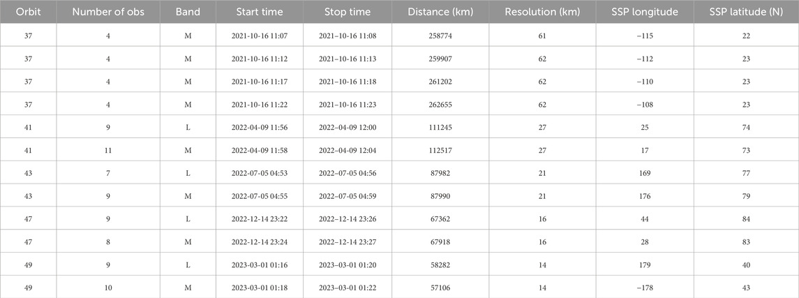
Table 1. List of observations of the M and L band used for this study. Distance, Sub-Spacecraft Point (SSP) longitude and latitude refers to the center of the observation period. Longitudes are West. The column “Resolution” indicates the minimum spatial resolution at the surface, in km.

Figure 1

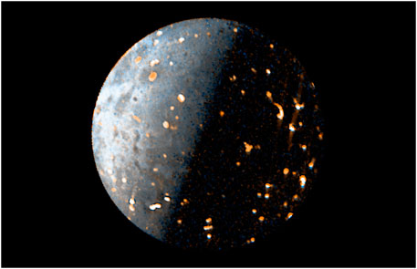
Figure 1. Io as seen by JIRAM during the 43rd orbit of Juno in a RGB composition of the L and M images (the M band is used for red channel, the L band is used for the blue channel; the green channel is an average between the M and L bands).

To enhance the signal-to-noise ratio and implement a super-resolution algorithm, the images captured both in the M- and L-band were stacked and superimposed. The method is the same used in Mura et al. (2020); here we just report the number of images of each observation (Table 1). The removal of reflected sunlight is performed in a subsequent step (see Section 3.1).

2.3 Limb fitting

The geometry of JIRAM observations can be reconstructed using routines and data provided by SPICE/NAIF (Acton, 1996). Generally, an accuracy comparable to the angular size of the JIRAM pixel is sufficient (for both the imager and spectrometer, which is approximately 237.8 µrad). However, in some cases, a significant deviation between the images and the reconstructed geometric information is found, suggesting the need for further correction. For example, this can occur in observations of Jupiter’s moons performed after a spacecraft reorientation, resulting in a slight wobbling phenomenon. Regardless of the reason, not investigated here, it is evident that a correction would be beneficial for the images used in this study.

A processing method similar to that used for analyzing the images in Mura et al. (2020) and Zambon et al. (2023) has been implemented. However, to avoid arbitrariness in interpreting the limb position, two substantial improvements have been introduced here. On Io’s dayside, especially in equatorial regions, Io can be quite bright, such that even one or two pixels outside the limb can have a significant radiance level, and radiance does not drop to zero sharply between pixels inside and outside the limb. This phenomenon gradually decreases toward the poles. Limb fitting on images without correcting for this effect would systematically shift the reconstructed limb toward the daylight direction. Therefore, an approximate and preliminary reconstruction of geometries was first carried out by using SPICE geometries only, and the image was corrected by applying a Lambertian lighting model; after this correction, the entire limb of the daylight side has an approximately constant radiance level.

The second modification involves introducing a routine that, to avoid the arbitrariness of the human operator’s choice of limb position, identifies it knowing that the dayside limb must be (after the correction mentioned in point 1) a semicircle with a known radius. As long as Io’s dimensions in pixels in JIRAM images do not exceed about 100 pixels, Io can be considered a sphere (for images of observations after those studied here, where Io is seen from closer, such as those in Juno’s orbits 51, 53, 57, and 58, an ellipsoid shape must be used). The routine finds the contour of constant radiance corresponding to a semicircle of the right radius and then determines the position of Io’s center. The improvement over limb fitting done by a human operator can be estimated on the order of one pixel, which is not much, but the method also has the advantage of being deterministic and repeatable.

Finally, as already mentioned, the images of each orbit are grouped and stacked. Limb fitting is performed on the already averaged super-image. Consequently, for orbits 41–49, we have 4 maps in the M band and 4 maps in the L band (as shown in Figure 2, see Section 3.1). The covered regions are very similar, and as a final check, it has been verified that the position of hotspots is the same in all 8 maps (see Supplementary Figure S4 for one example). Note that the coverage of the southern hemisphere is quite poor.

Figure 2

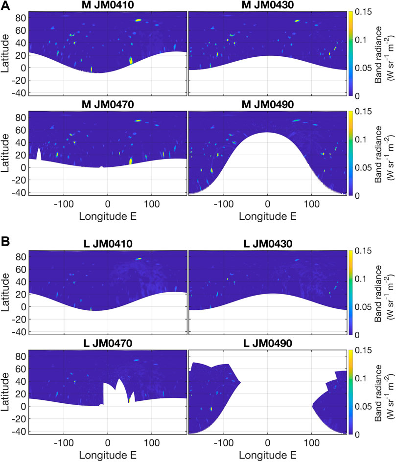
Figure 2. (A) Cylindrical equirectangular maps of the band radiance in the M filter for the orbits 41, 43, 47, and 49. (B) Cylindrical equirectangular maps of the band radiance in the L filter for the orbits 41, 43, 47, and 49.

3 Photometric models

3.1 Model for reflected sunlight

The radiation from the dayside of Io consists of both reflected sunlight and blackbody emission. Far from the hotspots, the equilibrium temperature expected for the surface of Io in its subsolar point within the thermal skin depth (of the order of a few mm) is −130 K (Rathbun et al., 2004), well below the detection threshold of JIRAM, so this component can be neglected. The reflected sunlight, on the other hand, must be considered as it is significantly bright at JIRAM wavelengths. Io is covered with a variety of different materials, including sulfur, sulfur dioxide frost, and various types of silicates, resulting in a diverse and complex surface. We found that an empirical model, similar to the Oren-Nayar one (Oren and Nayar, 1994), with respect to a simple Lambert model, provides a reliable way to describe the way light scatters off the dayside surface of Io. In this first version, spatial variability of albedo is not included in the model, i.e., albedo is assumed uniform (but different at different wavelengths). In the context of this model, a body surface roughness is represented by a statistical distribution of microfacets. These microfacets contribute to the scattered light in different directions, resulting in a diffuse reflection. The model, in fact, incorporates the roughness σ as a parameter (defined below). Furthermore, this model takes into account the incident light direction and the surface normal to calculate the intensity of reflected light. This accounts for the non-uniformity of Io’s surface and allows for more accurate rendering of its appearance under different lighting conditions.

Applying such a model to Io’s surface enables us to simulate the complex interactions of light with the various materials present. This allows generation of realistic values of reflected sunlight, that can be subtracted from the radiances measured by JIRAM to obtain the radiance due to Io’s hotspots only. Eqs 1–6 describe the model: θ_i and θ_r are the incident and reflection zenith angles (i.e., solar and emission angles), α and β are convenient angles defined by equations and 2:

$\alpha =\max \left({\theta }_i,{\theta }_r\right)(1)$

$\beta =\min \left({\theta }_i,{\theta }_r\right)(2)$

The roughness of the surface is given by the parameter σ, which is the standard deviation of the gradient of the surface elevation and ranges from 0 to ∞. For σ = 0, all facets lie in the same plane and the body is a perfect sphere. The horizontal projections of the incident and reflected beam (azimuthal angles) form an angle 𝜑 (𝜑_i - 𝜑_r). E₀ is the irradiance at the sub-solar point, and ε is a parameter to take into account the albedo. Then, three parameters C1, C2 and C3 are defined in the following way:

$C1=1-0.5\frac{{\sigma }^2}{{\sigma }^2+0.33}(3)$

$C2=\left\{\begin{array}{l}0.45\frac{{\sigma }^2}{{\sigma }^2+0.09}\sin \alpha ,\cos \phi >=0\\ 0.45\frac{{\sigma }^2}{{\sigma }^2+0.09}\left(\sin \alpha -{\left(2\frac{\beta }{\pi }\right)}^3\right),\cos \phi <0\end{array}\right.(4)$

$C3=0.125\frac{{\sigma }^2}{{\sigma }^2+0.09}{\left(4\alpha \frac{\beta }{{\pi }^2}\right)}^2(5)$

Now it is possible to define the two radiances, L1 (accounting for direct reflection) and L2 (accounting for multiple reflection of light between facets):

$L1=E_0{\left(\cos {\mathrm{\theta }}_i\right)}^e\frac{\mathrm{\epsilon }}{\mathrm{\pi }}\left(\mathrm{C}1+\mathrm{C}2\cos \phi \tan \beta +\mathrm{C}3\left(1-\left|\cos \phi \right|\right)\tan \left(\frac{\alpha +\beta }{2}\right)\right)(6)$

$L2=E_0{\left(\cos {\mathrm{\theta }}_i\right)}^{e}0.17\frac{{\mathrm{\epsilon }}^2}{\mathrm{\pi }}\frac{{\sigma }^2}{{\sigma }^2+0.13}\left(1-\cos \phi {\left(2\frac{\beta }{\pi }\right)}^2\right)(7)$

Finally, the radiance L of the light reflected by the surface is just:

$L=L1+L2(8)$

Note that we include a free parameter e, not present in the original version of the model, to allow a better fit of the data to the model. The model parameters are constrained using data taken from orbits 41, 43, 47 and 49 in both L and M bands. All hotspots have been removed from images to fit only the contribution from sunlight. In Supplementary Figures S1, S2 we show the data before the fit is performed; in Supplementary Figure S3 we show the model results, and the images after subtraction in one of the four cases. The parameters obtained from the fits are: ε = 0.19, σ = 0.88 and e = 0.90 for the L band; and ε = 0.34, σ = 1.5, e = 0.80 for the M band. Note that because we introduced an extra parameter e, the parameters ε and σ have values that do not reflect exactly the original meaning. In particular, the albedo or the Bond albedo should be calculated by using the formula. The result of this removal procedure, for orbits 41, 43, 47 and 49, is shown in Figure 2.

3.2 Model for emission angle variability of hotspot radiance

Some hotspots are localized within depressions (paterae), a situation in which the crater edges can effectively shield a portion of the emitted radiation as the emission angle becomes large. It is thus conceivable that Lambert’s cosine law may be an inaccurate approximation for the radiance variability of hotspots. In our dataset, we have a sample of four images taken at closely spaced time intervals (from orbit 37), during which the Juno probe has shifted its position slightly, albeit still significantly, relative to Io, presenting each hotspot under a different emission angle. Given the short duration of the overall observation (15 min), it is fully reasonable to assume that the observed radiance variability for each hotspot is solely attributable to changing observation conditions. Although no hotspot changes its emission angle over a very large range, the ensemble of hotspots covers an overall emission angle range practically from zero to 90°. Once the reflected solar component is removed, it is therefore quite straightforward to perform a best-fit of the radiance variability law as a function of the emission angle θ_r, which is assumed to be cos^α(θ_r), where the exponent α is a parameter that is presumably greater than one, due to the aforementioned concept (radiation emitted from depressed areas, and radiance that decreases faster than cos^α as α increases). Indeed, as shown in Figure 3, where the measured radiances are plotted on the x-axis and the estimated radiances on the y-axis, the law reproduces the variability of hotspots quite well, and the value of α obtained from the best fit (1.25), is indicative, as stated earlier, of a prevalence of emission from slightly depressed surfaces compared to the mean ground level. This concept has been proposed by de Kleer and de Pater (2016), who noted that correcting the radiance with cos¹ (θ_r) may be appropriate for some hot spots but not for others (see their Figure 12). It is important to have an accurate law for the emission angle, as in the continuation of this study, we will seek to assess the temporal variability of hotspots, but these are observed in situations of slightly different emission angles (orbits 41, 43, 47, and 49 have similar vantage points, but not exactly the same), and therefore precise correction is necessary. Because this effect is attributed to the shadowing of the hotter surface by colder patera walls, we can safely assume that the same function is valid for the L band as well.

Figure 3

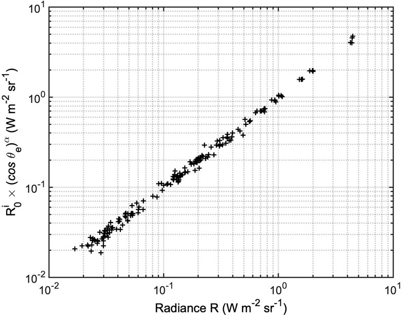
Figure 3. On the x-axis, the measured radiance integrated in the M band. On the y-axis, the modelled radiance assuming a cos^α(θ_r) law (θ_ris the emission angle, R₀ is the model radiance at θ_r= 0). The exponent α is found to be 1, 25. Note that each hotspot has its own R₀ⁱ.

4 Total power and spectral-derived temperatures

4.1 Retrieval of total power from the M band radiance

Io’s volcanic centers erupt lavas that are mafic in composition, based on their color and flow morphologies, and they have temperatures consistent with basaltic, or possibly ultramafic, compositions (e.g., Stansberry et al., 1997; Williams et al., 2001). Early analysis of Galileo data (McEwen et al., 1998; Davies et al., 2001) was suggestive of ultramafic lavas, which erupt at higher temperatures than basaltic lavas, up to −1800 K for the Pillan hotspot. However, subsequent analysis of the same data by Keszthelyi et al. (2007) indicates a lower limit of −1600 K, consistent with basaltic to lunar-like compositions. Mura et al. (2020), using JIRAM data, report a large range of temperature values that can fit the observed spectra (from 250 to more than 1,000 K). Some of these temperature values can be the effect of non-uniform filled pixel, that is they are somewhat an average of the hot and cold regions inside a pixel (where the hot regions are usually smaller but emitting more radiant power in comparison with colder regions). Note that the size of the pixel of the spectrometer of JIRAM is exactly equal to the pixel of the imager. Hence, we safely assume, or at least not exclude, that the same variability of detected temperature will be valid for the imager data. This is crucial when estimating the total power for a hotspot. A method to infer the total power from the M-band spectral radiance has been proposed and used in a recent paper (Davies et al., 2023). We note that, because of the variability of the detected temperature, this method may have large uncertainty. In Supplementary Figure S5 we show the ratio between the total power emitted from a black body, and the radiance at the M band center (for a grey body, with emissivity smaller than one, the ratio does not change). In the next Section, from the L/M ratio we will show that this range is completely covered by the data of our observation. A similar variability of temperatures can be found in Mura et al. (2020). In conclusion, estimating the total power only from the M band may lead to uncertainties up to one order of magnitude (and such uncertainty does not have a linear dependence with temperature); hence, we prefer to implement a 2-band total power estimation.

4.2 Estimating the temperature from the L/M ratio

The estimation of the hotspot temperature values on Io through the analysis of JIRAM spectra was first obtained by Mura et al. (2020). However, the data selected for our current study consists solely of dual-band images, because JIRAM spectra are not ideal for this study. In fact, as Juno gets closer to Io, Io gets larger (and faster) inside JIRAM’s field of view, and this implies that the spatial coverage of the spectrometer is reduced (after orbit 43, a malfunctioning of the de-spinning mirror prevented the use of the spectrometer anyway). However, it is possible to determine the temperature of a grey body source using only the radiance values in the L and M bands. As depicted in Fig. 6, the ratio between L and M band radiance has an almost linear relationship with temperature. This simulation employs the actual band ranges for L and M filters to integrate the Planck function at various temperatures. Notably, some uncertainties may exist in this estimation, such as potential variations in the emissivity at 3.45 and 4.8 µm. The provided value serves as an indicative average temperature within the image pixel, resembling an “effective temperature” as outlined in Eq. 1 of Lopes and Spencer. (2007a). It is crucial to acknowledge that this assumes uniform emissivity across the ∼3–∼5 µm range (i.e., a grey body in this spectral range), which might not be the case. Consequently, the temperature derived in this manner can be less precise than that derived from the full spectrum. Nevertheless, this estimation surpasses the accuracy of using a single band, which is influenced by factors such as the fill factor, indicating the partial occupancy of a pixel by the source, and uncertainties in emissivity magnitude.

This method requires that each hotspot has a radiance spectrum that is indicative of one temperature only: as a matter of fact, most spectra in Figure 3A of Mura et al. (2020) do not show bimodal distributions. However, to evaluate the significance of the temperature that is estimated in this way, one can consider the background temperature and the imagers’ minimum detectable signal, which at 1 s of exposure time is 5 10⁻⁶ W sr⁻¹m⁻² and increases as the exposure time decreases. Such value, in the M band and for usual exposure times, corresponds to about 150 K; in practice, JIRAM would be able to measure the surface temperature in regions away from hotspots only if it could observe areas completely free of hotspots with very long exposure times and with high resolution. However, this did not occur during the observational campaign. In practice, any temperature above 500 K and any filling factor greater than 1 in ten thousand cause the radiance in the 2–5 micron range, and therefore especially in the individual L and M bands, not to be influenced by anything other than the hottest source. Consequently, our temperature retrieval is possible. Once the temperature retrieval is performed, it is possible to calculate the filling factor that provides the correct values for the two radiances, L and M, and verify that the found value is within an acceptable range (i.e., not fitting the temperature of a too small portion of the pixel).

After the temperature of a hotspot is estimated (i.e., the temperature of a grey body that best fit the radiance in the two bands) it is trivial to compute the total power by integrating the Planck function (over the wavelength and solid angle) and multiplying by the hotspot area (see next Section for details).

5 The temporal variability of hotspots power output

In Table 2 we show a list of hotspots from observations during Juno orbits 41, 43, 47, and 49. We identify the names of these hotspots by comparing their location with those reported in the tables by Zambon et al. (2023) and Davies et al. (2023). “Unnamed” hotspots are known hotspots for which there is no official name. “Unrecognized” hotspots are those for which it is difficult to identify a previously known candidate (these may include new detections). Peak radiances in the M and L band are reported in the respective columns, as well as the location (latitude and longitude). In Table 3, a similar list of hotspots is shown, in this case the total output in the M band and L band is estimated by integrating the radiance over the hotspots’ apparent area. For each hotspot, this value is estimated by computing the spatial full-width half maximum contour line around the peak, counting the pixels in this region, and considering the distance between Juno and Io at the time of the observation, and the solid angle of the IFOV (237.8 µrad by 237.8 µrad). Finally, the emission angle dependence is corrected according to the formula given in Section 3.2.

Table 2

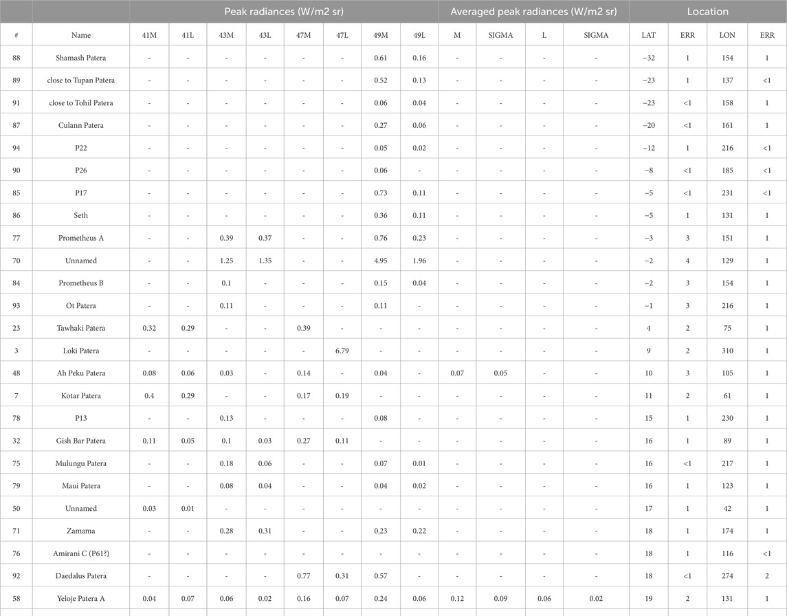
Table 2. List of hotspots from observations during Juno orbits 41, 43, 47, and 49. “41M” means identification in orbit 41 in the M band, “41L” is for the L band, etc. Longitudes are West. Names are consistent with tables from Zambon et al., 2023; Davies et al., 2023. Unnamed hotspots are known hotspots for which there is no official name. HS 72 and 74 are very close but distinct. Hotspots have been sorted by increasing latitude; the first column indicates the original number in the database.

Table 3

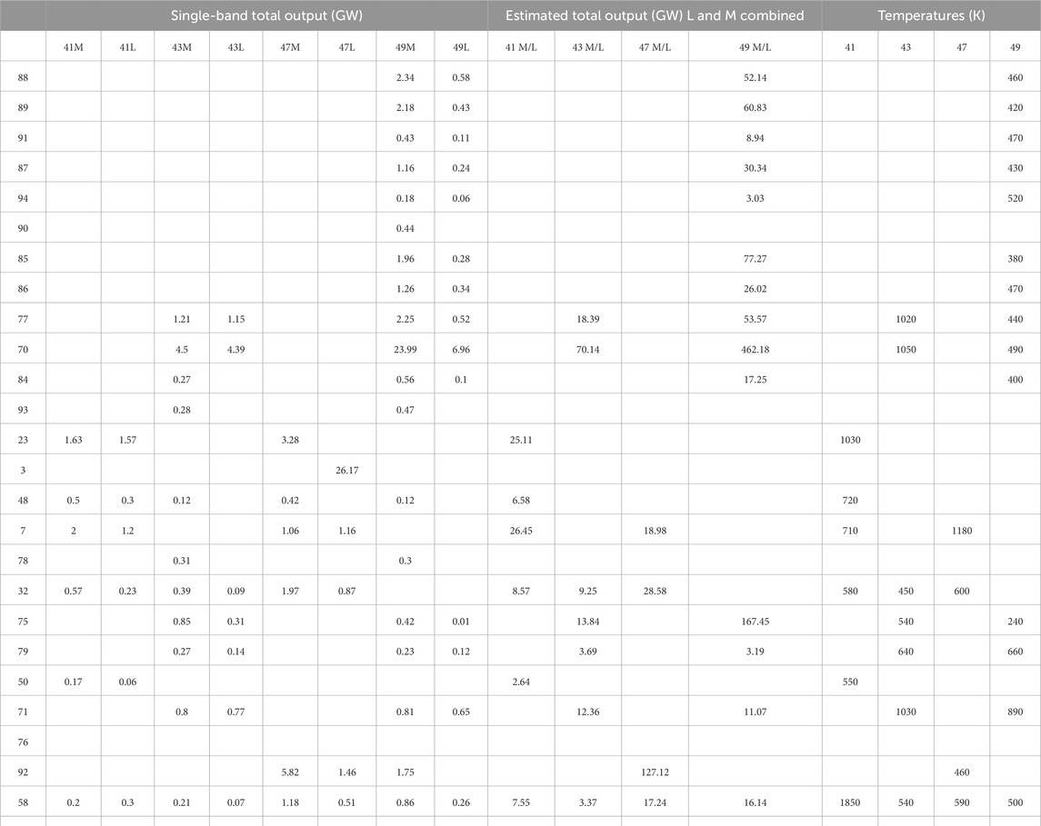
Table 3. Total power output in the M band, L band, estimated total, and retrieved temperature (to convert the single-band total output to units of GW/µm/sr, multiply the L band values in columns 3, 5, 7, and 9 by 1.06, and the M-band values in columns 2, 4, 6 and 8 by 0.64). Numbers and sorting are consistent with Table 2.

In Table 3 we also report the estimation of the total power output (by using both the L and M bands, as explained in Section 4.2) and of the temperature.

In Figure 4 we plot the mean power output (blue line, in GW) and temperature (red line, in K) as a function of latitude. There is no clear latitudinal trend in terms of total output because, even if the curve shows a maximum close to the equator, there is also a secondary maximum in the North polar regions. These results, by themselves, are not in disagreement with those by Davies et al., 2023 (see Section 6 for a detailed discussion).

Figure 4

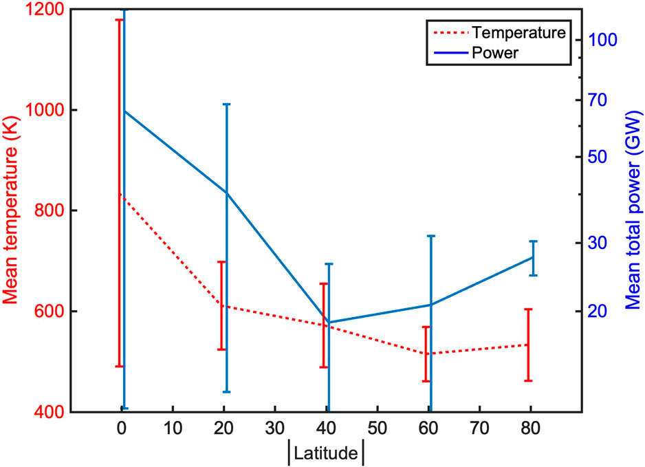
Figure 4. Mean power output (blue line, in W, scale to the right) and mean temperature (red dashed line, in K, scale to the left) as a function of the absolute value of the latitude. Hotspots have been binned in groups according to their absolute value of the latitude (from 0° to 10°, from 10° to 30°, etc); note that there are very few data points from the southern region. Error bars are the standard deviation of the data in each bin.

The temperature plot, on the other hand, seems to indicate that the equatorial hotspots have higher temperature, but the standard deviation is quite large, suggesting that more data will be necessary to draw a final conclusion. In particular, the coverage of the southern hemisphere is quite poor (Figure 2). Once JIRAM will be able to take high-resolution images of these regions, in 2024, it will be possible to check whether this hypothesized trend of the North pole to have lower hotspot temperature is confirmed also for the South pole.

To quantify the temporal variability of the hotspots, we took the standard deviation of the total power in the M band divided by the mean of the total power in the M band. We decide to use only the M band for several reasons. First, the L band, having generally lower radiance, is more prone to larger relative errors. Also, in the L band there is stronger reflected sunlight, so even after applying a photometric function some residuals may remain in the data. While using two spectral bands for estimating the variability increases the accuracy of the derived trends, it also has the effect of introducing two instrumental uncertainties instead of one. Finally, the hotspot coverage by the M band is larger and not exactly the same of that for the L band, so if we were to use only hotspots with dual imaging, we would have a significantly smaller sample of hotspots.

In any case, a hotspot that varies its total power output also varies its radiance in every part of the spectrum, including the M band. Since the result we present is normalized to the average radiance over the period, the uncertainty in the correlation between total power and M-band power (see Section 4.1) is removed by this normalization, and therefore, there is no risk of introducing significant systematic biases (instead, it is appropriate to use both bands when estimating the total output because the use of the M band alone is prone to systematic biases, as discussed before).

In Figure 5 we show the temporal variability of the four hotspots that have the largest variability among our sample (Asis P., Volund P., Girru P. and Susanoo P.). The power output has beenm normalized to the average of the 94 hotspots; the blue line shows the average of all hotspots as a function of time (it is almost constantly equal to one, that is on average all hotspots did not change the power output during 1 year), and the uncertainty is equal to 0.4, because each hotspot, singularly, varied its power output of about 40%. The other four lines are the power output for the four significant cases mentioned above. These four hotspots show a variation in time that exceed that of the others, and are all located between the equator and 45°N.

Figure 5

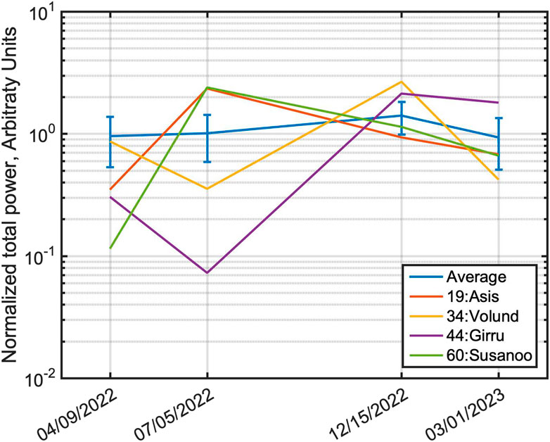
Figure 5. variation of the power output in the M band for 4 significant cases. The power output has been normalized to the average of the 94 hotspots; the blue line shows the average of all hotspots function of time (it is almost constantly equal to one, that is on average all hotspots did not change the power output during 1 year), and the error bar is equal to 0.4, because each hotspot, singularly, varied its power output of about 40% (this is the average of the variability, see text for more information). The other four lines are the power output for four significant cases: Asis P., Volund P., Girru P. and Susanoo P. These hotspots show a variation in time that is much larger than all the others.

Finally, we computed the relative standard deviation of the M-band power output for all hotspots, and then we binned these values in groups of 10 degrees of latitude (as in Figure 4, the absolute value of the latitude is used). The result is shown in Figure 6: there is evidence that the equatorial hotspots have a larger temporal variability, and this variability gradually decreases towards the poles.

Figure 6

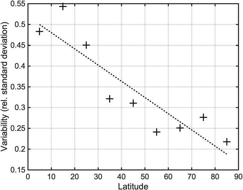
Figure 6. Variability of M-band power output function of latitude. On the y-axis, the relative (i.e., normalized) standard deviation of the power output is shown, averaged over all hotspots in bins of 10 degrees of latitude. The dashed line is a linear best-fit of data.

6 Summary and conclusions

In this study we present:

1) a new photometric model for the dayside reflected sunlight, which takes advantage of the unique opportunity, given by Juno, to observe Io from higher phase angles and latitudes than Earth-based observations;

2) an accurate model for the hotspots’ emission angle dependence, which is necessary to disentangle the observed radiance variability due to changing vantage point from that due to physical variability of the hotspots emitted radiance;

3) an improved mapping of hotspots, especially at high latitudes;

4) and, as the primary outcome of this study, a characterization of Io’s hotspot temporal variability, showing that low latitude hotspots have more intense temporal variability.

Many studies focus on spatial variability (Davesi et al., 2023, Pettine et al., submitted), but, at least concerning JIRAM data, spatial variability cannot be computed without aggregating data taken at considerably different times. Therefore, it is important to estimate temporal variability since it can influence the conclusions of studies like the aforementioned ones. Alternatively, to study spatial variability, Earth-based data can be used (Marchis et al., 2002; Marchis et al., 2005; de Kleer et al., 2014; de Kleer and de Pater, 2016; Cantrall et al., 2018). However, in this case, there is a strong correlation between latitude and emission angle, which, for polar regions, could affect the conclusions. For example, one can consider the dependence law of radiance on emission angle, which differs from the one used so far (a cosine law, as in Davies et al., 2023). The study of spatial and temporal distribution of Io’s power output was already performed with NASA/Galileo data (Lopes-Gautier et al., 1999; Rathbun et al., 2004), and with New Horizons data (Rathbun et al., 2014). However, Galileo and New Horizon observations do not allow a complete and detailed coverage of Io’s polar regions due to their equatorial orbit (Smith, 1979; Perry et al., 2007; Davies et al., 2001; Veeder et al., 2012; Tsang et al., 2014; Rathbun et al., 2018).

To monitor the power output of hotspots, it is necessary to remove the solar reflected light. This requires a map of surface albedo accompanied by a photometric model. For now, we have just produced a photometric model assuming a uniform albedo, which is a first approximation. In the future, we aim to produce an albedo map for the entire surface of Io.

It should be considered that constraining a heating model in the asthenosphere with the power output of hotspots by latitude has the intrinsic problem that a minority of hotspots contributes to the majority of the power output, at least in the spectral range we consider (not considering Loki, the 10 most powerful hotspots contribute to more than 50% of total power in both the L and M bands, in the region considered in this paper). For instance, in Davies et al. (2023), a calculation of power output density is done for “polar regions” (latitude above 60°) and “equatorial regions.” It is interesting to consider that, using the same data, but setting such reference latitude at different values leads to very different results, due to the fact that a few volcanoes have a large specific weight in the calculation of the radiance density. This is quite puzzling, because heating as a function of latitude (for asthenospheric tidal heating models) shows a smooth trend, and thus the same pole/equator asymmetry should be seen for any definition of the latitude boundary.

The dependence of temporal variability of hotspots on latitude, on the other hand, is somewhat more regular and seems to support the results of Davies et al. (2023), and our results agree with the conclusions of Cantrall et al. (2018). However, it must be remembered that theoretical models do not explicitly state that polar regions, besides having lower output, should have less temporal variability. This is only an inductive reasoning that would require more theoretical foundation. However, it has been suggested by McEwen et al. (2000) that low- and high-latitude volcanoes may be of different types; these authors reported that far from the equator, the eruptions are mostly short-lived. This should be combined with our results that there is less activity (less frequency of eruptions) far from the equator. We conclude that it will be necessary, in the near future, to check if the same variability exists for hotspots in the southern polar region. This would give more strength to the results presented here and prompt an investigation into whether there is sufficient data to constrain a theoretical model. As the Juno mission progresses, the observation of the southern hemisphere of Io becomes increasingly feasible due to favorable orbit conditions. In orbits 53, 55, 57, 58, and 60 (late 2023/early 2024), JIRAM is expected to have a significant opportunity to observe Io with a pixel resolution down to 3 km. This will result in a substantial and unique database, particularly for the polar regions, which cannot be achieved through Earth-based telescopic observations. In this respect, or results prepare for the analysis of future Juno/JIRAM observations of Io.

Data availability statement

The original contributions presented in the study are included in the article/Supplementary material, further inquiries can be directed to the corresponding author.

Author contributions

AM: Validation, Writing–original draft, Writing–review and editing, Conceptualization, Data curation, Formal Analysis, Investigation, Methodology, Supervision, Visualization. FZ: Writing–review and editing, Investigation. FT: Writing–review and editing, Investigation. RL: Writing–review and editing, Supervision. JR: Writing–review and editing, Supervision. MP: Writing–review and editing. AA: Investigation, Supervision, Validation, Writing–review and editing. Francesca FA: Writing–review and editing. MC: Writing–review and editing. AC: Investigation, Writing–review and editing. GF: Investigation, Writing–review and editing. DG: Investigation, Writing–review and editing. RN: Data curation, Investigation, Writing–review and editing. AM: Writing–review and editing. GP: Conceptualization, Investigation, Writing–review and editing. CP: Investigation, Writing–review and editing. RS: Conceptualization, Investigation, Writing–review and editing. GS: Investigation, Writing–review and editing. DT: Investigation, Writing–review and editing.

Funding

The author(s) declare that no financial support was received for the research, authorship, and/or publication of this article.

Acknowledgments

We thank ASI (Agenzia Spaziale Italiana) for support of the JIRAM contribution to the Juno mission; JIRAM is funded by the ASI–INAF Addendum n. 2016-23-H.3-2023 to grant 2016-23-H.0. Part of this work was carried out at the Jet Propulsion Laboratory, California Institute of Technology, under contract with NASA.

Conflict of interest

The authors declare that the research was conducted in the absence of any commercial or financial relationships that could be construed as a potential conflict of interest.

The author(s) declared that they were an editorial board member of Frontiers, at the time of submission. This had no impact on the peer review process and the final decision.

The reviewer IDP declared a past co-authorship with the authors AM and FT to the handling Editor.

Publisher’s note

All claims expressed in this article are solely those of the authors and do not necessarily represent those of their affiliated organizations, or those of the publisher, the editors and the reviewers. Any product that may be evaluated in this article, or claim that may be made by its manufacturer, is not guaranteed or endorsed by the publisher.

Supplementary material

The Supplementary Material for this article can be found online at: https://www.frontiersin.org/articles/10.3389/fspas.2024.1369472/full#supplementary-material

SUPPLEMENTARY FIGURE S1Four M-band images of Io (spectral radiance at 4.78 μm), taken during Juno’s orbit 37 (see Table 1 for details). The positions of the North pole and the meridian 120E/240W are superimposed in blue.

SUPPLEMENTARY FIGURE S2Four L-band images and 4 M-band images of Io (spectral radiances at 3.45 and 4.78 μm), taken during Juno‘s orbit 41, 43, 47 and 49 (see Table 1 for details). The positions of the North pole and the meridians 30W or 180W are superimposed in blue.

SUPPLEMENTARY FIGURE S3Left: example of one L-band image of Io before sunlight subtraction (left); dark dots are locations of hotspots, not considered for sunlight subtraction. Center: model for sunlight correction. Right: L-band image after sunlight subtraction.

SUPPLEMENTARY FIGURE S4Example of the identification of a hotspot in 4 orbits and 2 bands (red labels in the lower right corner indicate the orbit and the band). Numbers are consistent with column 1 in tables 2 and 3; white dashed lines are parallels (every 5°, see bottom-right panel for latitudes); red dashed lines are meridians (every 5°, see bottom-right panel for longitudes - West).

SUPPLEMENTARY FIGURE S5Ratio between the total radiance over the band radiance in the M band as a function of temperature.

SUPPLEMENTARY FIGURE S6Ratio between the L and M band radiance as a function of the temperature of a grey body source (emissivity between 3 and 5 μm is assumed constant).

References

Acton, C. H. (1996). Ancillary data services of NASA’s navigation and ancillary information facility. Planet. Space. Sci. 44 (1), 65–70. doi:10.1016/0032-0633(95)00107-7

CrossRef Full Text | Google Scholar

Adriani, A., Coradini, A., Filacchione, G., Lonnie, J. I., Bini, A., Pasqui, C., et al. (2008). JIRAM, the image spectrometer in the near infrared on board the Juno mission to Jupiter. Astrobiology 8 (3), 613–622. doi:10.1089/ast.2007.0167

PubMed Abstract | CrossRef Full Text | Google Scholar

Adriani, A., Filacchione, G., Di Iorio, T., Turrini, D., Noschese, R., Cicchetti, A., et al. (2014). JIRAM, the jovian infrared auroral mapper. Space Sci. Rev. 213, 393–446. doi:10.1007/s11214-014-0094-y

CrossRef Full Text | Google Scholar

Adriani, A., Moriconi, M. L., Mura, A., Tosi, F., Sindoni, G., Noschese, R., et al. (2016). Juno’s Earth flyby: the Jovian infrared Auroral Mapper preliminary results. Astrophys. Space Sci. 361 (8), 272. article id.272. doi:10.1007/s10509-016-2842-9

CrossRef Full Text | Google Scholar

Bolton, S. J., Adriani, A., Adumitroaie, V., Allison, M., Anderson, J., Atreya, S., et al. (2017). Jupiter’s interior and deep atmosphere: the initial Pole-to-Pole passes with the Juno spacecraft : 821–825.

PubMed Abstract | CrossRef Full Text | Google Scholar

Cantrall, C., de Kleer, K., de Pater, I., Williams, D. A., and DaviesNelson, A. G. D. (2018). Variability and geologic associations of volcanic activity on Io in 2001-2016. Icarus 312, 267–294. doi:10.1016/j.icarus.2018.04.007

CrossRef Full Text | Google Scholar

Carlson, R. W., Kargel, J. S., Doute, S., Soderblom, L. A., and Dalton, J. B. (2007). “Io’s surface composition,” in Io after Galileo. Praxis publishing company. Editors R. Lopes, and J. R. Spencer (China: Springer-Verlag).

Google Scholar

Carlson, R. W., Smythe, W. D., Lopes-Gautier, R. M. C., Davies, A. G., Kamp, L. W., Mosher, J. A., et al. (1997). Distribution of sulfur dioxide and other infrared absorbers on the surface of Io. Geophys. Res. Lett. 24, 2479–2490. doi:10.1029/97GL02609

CrossRef Full Text | Google Scholar

Davies, A. G., Keszthelyi, L. P., Williams, D., Phillips, C., McEwen, A. S., Lopes, R., et al. (2001). Thermal signature, eruption style and eruption evolution at Pele and Pillan on Io. J. Geophys. Res. 106, 33079–33103. doi:10.1029/2000je001357

CrossRef Full Text | Google Scholar

Davies, A. G., Perry, J. E., Williams, D. A., and Nelson, D. M. (2023). Io’s polar volcanic thermal emission indicative of magma ocean and shallow tidal heating models. Nat. Astron 8, 94–100. doi:10.1038/s41550-023-02123-5

CrossRef Full Text | Google Scholar

de Kleer, K., and de Pater, I. (2016). Time Variability of Io's volcanic activity from near-IR adaptive optics observations on 100 nights in 2013-2015. Icarus 280, 378–404. doi:10.1016/j.icarus.2016.06.019

CrossRef Full Text | Google Scholar

de Kleer, K., and de Pater, I. (2017). Io’s Loki Patera: modeling of three brightening events in 2013–2016. Icarus 289, 181–198. doi:10.1016/j.icarus.2017.01.038

CrossRef Full Text | Google Scholar

de Kleer, K., de Pater, I., Ádámkovics, M., and Davies, A. G. (2014). Near-infrared monitoring of Io and detection of a violent outburst on 29 August 2013. Icarus 242, 352–364. doi:10.1016/j.icarus.2014.06.006

CrossRef Full Text | Google Scholar

de Pater, I., Davies, A. G., and Marchis, F. (2016b). Keck observations of eruptions on Io in 2003-2005. Icarus 274, 284–296. doi:10.1016/j.icarus.2015.12.054

CrossRef Full Text | Google Scholar

de Pater, I., de Kleer, K., Davies, A. G., and Ádámkovics, M. (2017). Three decades of Loki patera observations. Icarus 297, 265–281. doi:10.1016/j.icarus.2017.03.016

CrossRef Full Text | Google Scholar

de Pater, I., Laver, C., Davies, A. G., de Kleer, K., Williams, D. A., Howell, R. R., et al. (2016a). Io: eruptions at pillan, and the time evolution of pele and pillan from 1996 to 2015. Icarus 264, 198–212. doi:10.1016/j.icarus.2015.09.006

CrossRef Full Text | Google Scholar

Kervazo, M., Tobie, G., Choblet, G., Dumoulin, C., and Běhounková, M. (2022). Inferring Io’s interior from tidal monitoring. Icarus 373, 114737. doi:10.1016/j.icarus.2021.114737

CrossRef Full Text | Google Scholar

Keszthelyi, L., Jaeger, W., Milazzo, M., Radebaugh, J., Davies, A. G., and Mitchell, K. L. (2007). New estimates for Io eruption temperatures: implications for the interior. Icarus, 192(2), pp.491–502. doi:10.1016/j.icarus.2007.07.008

CrossRef Full Text | Google Scholar

Lopes, R., Kamp, L. W., Smythe, W. D., Mouginis-Mark, P., Kargel, J., Radebaugh, J., et al. (2004). Lava lakes on Io: observations of Io's volcanic activity from Galileo NIMS during the 2001 fly-bys. Icarus 169/1, 140–174. doi:10.1016/j.icarus.2003.11.013

CrossRef Full Text | Google Scholar

R. Lopes, and J. R. Spencer (2007b). Io after Galileo (USA: Praxis Publishing Company (Springer-Verlag).

Google Scholar

Lopes, R., and Williams, D. (2005). Io after Galileo. Rep. Prog. Phys. Inst. Phys. Publ. 68, 303–340. doi:10.1088/0034-4885/68/2/r02

CrossRef Full Text | Google Scholar

Lopes, R. M., and Spencer, J. R. (2007a). Io after Galileo. Berlin: Springer.

Google Scholar

Lopes-Gautier, R., McEwen, A. S., Smythe, W., Geissler, P., Kamp, L., Davies, A. G., et al. (1999). Active volcanism on Io: global distribution and variations in activity. Icarus 140 (2), 243–264. doi:10.1006/icar.1999.6129

CrossRef Full Text | Google Scholar

Marchis, F., dePater, I., Davies, A. G., Roe, H. G., Fusco, T., Le Mignant, D., et al. (2002). High-resolution keck adaptive optics imaging of violent volcanic activity on Io. Icarus 160, 124–131. doi:10.1006/icar.2002.6955

CrossRef Full Text | Google Scholar

Marchis, F., Le Mignant, D., Chaffee, F. H., Davies, A. G., Kwok, S. H., Prangé, R., et al. (2005). Keck AO survey of Io global volcanic activity between 2 and 5 μm. Icarus 176, 96–122. doi:10.1016/j.icarus.2004.12.014

CrossRef Full Text | Google Scholar

Masursky, H., Schaber, G. G., Soderblom, L. A., and Strom, R. G. (1979). Preliminary geological mapping of Io. Nature 280, 725–729. doi:10.1038/280725b0

CrossRef Full Text | Google Scholar

McEwen, A. S., Belton, M. J. S., Breneman, H. H., Fagents, S. A., Geissler, P., Greeley, R., et al. (2000). Galileo at Io: results from high-resolution imaging. Science 288 (5469), 1193–1198. doi:10.1126/science.288.5469.1193

PubMed Abstract | CrossRef Full Text | Google Scholar

McEwen, A. S., Keszthelyi, L., Spencer, J. R., Schubert, G., Matson, D. L., Lopes-Gautier, R., et al. (1998). High-temperature silicate volcanism on jupiter's moon Io. Science 281, 87–90. doi:10.1126/science.281.5373.87

PubMed Abstract | CrossRef Full Text | Google Scholar

Morabito, L. A., Synnot, S. P., Kupfermann, P. N., and Collins, S. A. (1979). Discovery of currently active extra-terrestrial volcanism. Science 204, 972. doi:10.1126/science.204.4396.972.a

PubMed Abstract | CrossRef Full Text | Google Scholar

Mura, A., Adriani, A., Tosi, F., Lopes, R. M. C., Sindoni, G., Filacchione, G., et al. (2020). Infrared observations of Io from Juno. Icarus 341, 113607. doi:10.1016/j.icarus.2019.113607

CrossRef Full Text | Google Scholar

Oren, M., and Nayar, S. K. (1994). “Generalization of Lambert’s reflectance model,” in Proceedings of the 21st annual conference on Computer graphics and interactive techniques - SIGGRAPH '94, USA, 24-29 July 1994 (ACM Press).

Google Scholar

Peale, S. J., Cassen, P., and Reynolds, R. T. (1979). Melting of Io by tidal dissipation. Science 203, 892–894. doi:10.1126/science.203.4383.892

PubMed Abstract | CrossRef Full Text | Google Scholar

Rathbun, J., Spencer, J. R., Lopes, R. M., and Howell, R. R. (2014). Io’s active volcanoes during the new Horizons era: insights from new Horizons imaging. Icarus 231, 261–272. doi:10.1016/j.icarus.2013.12.002

CrossRef Full Text | Google Scholar

Rathbun, J. A., Lopes, R. M. C., and Spencer, J. R. (2018). The global distribution of active Ionian volcanoes and implications for tidal heating models. AJ 156, 207. doi:10.3847/1538-3881/aae370

CrossRef Full Text | Google Scholar

Rathbun, J. A., Spencer, J. R., Tamppari, L. K., Martin, T., Barnard, L., and Travis, L. (2004). Mapping of Io’s thermal radiation by the Galileo photopolarimeter–radiometer (PPR) instrument. Icarus 169, 127–139. doi:10.1016/j.icarus.2003.12.021

CrossRef Full Text | Google Scholar

Ross, M. N., and Schubert, G. (1985). Tidally forced viscous heating in a partially molten Io. Icarus 64 (3), 391–400. doi:10.1016/0019-1035(85)90063-6

CrossRef Full Text | Google Scholar

Segatz, M., Spohn, T., Ross, M. N., and Schubert, G. (1988). Tidal dissipation, surface heat flow, and figure of viscoelastic models of Io. Icarus 75 (2), 187–206. doi:10.1016/0019-1035(88)90001-2

CrossRef Full Text | Google Scholar

Smith, B. A., Soderblom, L. A., Johnson, T. V., Ingersoll, A. P., Collins, S. A., Shoemaker, E. M., et al. (1979). The Jupiter system through the eyes of Voyager 1. Science 204, 951–972. doi:10.1126/science.204.4396.951

PubMed Abstract | CrossRef Full Text | Google Scholar

Spencer, J. R., Jessup, K. L., McGrath, M. A., Ballester, G. E., and Yelle, R. (2000). Discovery of gaseous S₂ in Io’s Pele plume. Science 288, 1208–1210. doi:10.1126/science.288.5469.1208

PubMed Abstract | CrossRef Full Text | Google Scholar

Spencer, J. R., and Schneider, N. M. (1996). Io on the eve of the Galileo mission. Annu. Rev. Earth Planet. Sci. 24, 125–190. doi:10.1146/annurev.earth.24.1.125

CrossRef Full Text | Google Scholar

Spencer, J. R., Stern, S. A., Cheng, A. F., Weaver, H. A., Reuter, D. C., Retherford, K., et al. (2007). Io volcanism seen by new Horizons: a major eruption of the tvashtar volcano. Science 318, 240–243. doi:10.1126/science.1147621

PubMed Abstract | CrossRef Full Text | Google Scholar

Strom, R. G., and Schneider, N. M. (1982). Volcanic eruption plumes on Io, satellites of jupiter. (A83-16226 04-91). Tucson, AZ: University of Arizona Press, 598–633.

Google Scholar

Trafton, L. M., Lester, D. F., Ramseyer, T. F., Salama, F., Sandford, S. A., and Allamandola, L. J. (1991). A new class of absorption feature in lo's near-infrared spectrum. Icarus 89, 264–276. doi:10.1016/0019-1035(91)90178-V

PubMed Abstract | CrossRef Full Text | Google Scholar

Tsang, C., Rathbun, J., Spencer, J., Hesman, B., and Abramov, O. (2014). Io's hotspots in the near-infrared detected by LEISA during the new Horizons flyby. J. Geophys. Res. Planets 119, 2222–2238. doi:10.1002/2014JE004670

CrossRef Full Text | Google Scholar

Tyler, R. H., Henning, W. G., and Hamilton, C. W. (2015). Tidal heating in a magma ocean within Jupiter’s moon Io. Astrophys. J. Suppl. Ser. 218 (22), 22. doi:10.1088/0067-0049/218/2/22

CrossRef Full Text | Google Scholar

Veeder, G. J., Davies, A. G., Matson, D. L., and Johnson, T. V. (2009). Io: heat flow from dark volcanic fields. Icarus 204, 239–253. doi:10.1016/j.icarus.2009.06.027

CrossRef Full Text | Google Scholar

Veeder, G. J., Davies, A. G., Matson, D. L., Johnson, T. V., Williams, D. A., and Radebaugh, J. (2012). Io: volcanic thermal sources and global heat flow. Icarus 219, 701–722. doi:10.1016/j.icarus.2012.04.004

CrossRef Full Text | Google Scholar

Veeder, G. J., Davies, A. G., Matson, D. L., Johnson, T. V., Williams, D. A., and Radebaugh, J. (2015). Io: heat flow from small volcanic features. Icarus 245, 379–410. doi:10.1016/j.icarus.2014.07.028

CrossRef Full Text | Google Scholar

Veeder, G. J., Matson, D. L., Johnson, T. V., Blaney, D. L., and Goguen, J. D. (1994). Io’s heat flow from infrared radiometry: 1983--1993. J. Geophys. Res. 99, 17095–17162. doi:10.1029/94je00637

CrossRef Full Text | Google Scholar

Williams, D. A., Greeley, R., Lopes-Gautier, R., and Davies, A. G. (2001). Evaluation of sulfur flow emplacement on Io from Galileo data and numerical modeling. J. Geophys. Res. 106, 174.

CrossRef Full Text | Google Scholar

Zambon, F., Mura, A., Lopes, R. M. C., Rathbun, J., Tosi, F., Sordini, R., et al. (2023). Io hot spot distribution detected by Juno/JIRAM. Geophys. Res. Lett. 50, e2022GL100597. doi:10.1029/2022GL100597

CrossRef Full Text | Google Scholar